Understanding Relative and Absolute Change in Discontinuous Growth Models

Abstract

Organizational researchers routinely have access to repeated measures from numerous time periods punctuated by one or more discontinuities. Discontinuities may be planned, such as when a researcher introduces an unexpected change in the context of a skill acquisition task. Alternatively, discontinuities may be unplanned, such as when a natural disaster or economic event occurs during an ongoing data collection. In this article, we build off the basic discontinuous growth model and illustrate how alternative specifications of time-related variables allow one to examine relative versus absolute change in transition and post-transition slopes. Our examples focus on interpreting time-varying covariates in a variety of situations (multiple discontinuities, linear and quadratic models, and models where discontinuities occur at different times). We show that the ability to test relative and absolute differences provides a high degree of precision in terms of specifying and testing hypotheses.

Keywords

change multilevel models mixed-effects models discontinuity events

Organizational researchers routinely have access to repeated measures from numerous time periods punctuated by one or more discontinuities. Several examples serve as illustrations. Kim and Ployhart (2014) examined 12 years of firm performance data from 359 firms and demonstrated that a general trend of increased firm performance was altered by the great recession. Kramer and Chung (2015) analyzed BMI data over 16 years from 4,264 working respondents and showed that a trend of BMI increase over time was mitigated by factors such as increased work responsibility. Bliese, McGurk, Thomas, Balkin, and Wesensten (2007) collected 26 days of sleep data using wrist-worn actigraphs from 77 Army cadets and demonstrated that sleep time increased as participants habituated to sleeping in a barracks environment but then decreased when cadets moved to a field exercise. Lang and Bliese (2009) collected 12 waves of data from 184 participants on a complex computer-based task and modeled individual differences in performance when participants encountered an unexpected task change. Finally, Aguinis et al. (2010) examined the scientific productivity of 58 journal editors over several decades of the editors’ professional lives and modeled two discontinuities—the first when the editorship began and the second when it ended.

A combination of numerous measures interrupted by one or more discontinuities is common in contexts beyond the aforementioned examples. Researchers frequently use automated methods to collect repeated measures over a period of weeks in experience sampling methodology (ESM) designs—designs that can potentially track patterns within a work week (e.g., documenting increased levels of emotional exhaustion) and examine how patterns might be interrupted by events such as weekend recovery periods. Similarly, increasingly sophisticated sensor platforms allow researchers to collect real-time physiological data and examine the impact of events such as encounters with team members or responses to demanding tasks (see Kozlowski, Chao, Chang, & Fernandez, 2016). As another example, broad efforts to implement electronic recording keeping in health care (Blumenthal & Tavenner, 2010) are producing longitudinal databases that will increasingly allow researchers to examine how events such as experiencing a work-related trauma or being exposed to a natural disaster influence health trajectories. Finally, many organizations are routinely collecting employee and customer data allowing researchers to examine how planned or unplanned events relate to variables such as customer satisfaction or employee turnover. Indeed, in education research, Raudenbush (2009) notes that an “exciting new genre of research is now possible because more and more states and school districts … have assembled sophisticated longitudinal data systems” allowing researchers to examine the impact of policy changes.

Table 1 provides additional examples of published topic areas involving change processes that potentially entail numerous observations and discontinuities. The topics include retirement (Wang, 2007), transitions into and out of unemployment (Lucas, Clark, Georgellis, & Diener, 2004), mergers and acquisitions (Barkema & Schijven, 2008; Marquis & Huang, 2010), patterns of job satisfaction (honeymoons and hangovers) associated with job changes (Boswell, Shipp, Payne, & Culbertson, 2009), and studies of furloughs on employee burnout and recovery (Halbesleben, Wheeler, & Paustian-Underdahl, 2013). The studies in Table 1 used a variety of appropriate analytic techniques to understand the ubiquitous phenomenon of discontinuous change. We believe, however, that discontinuous growth models can augment existing techniques and enhance researchers’ ability to study discontinuous change.¹

Table 1.

Examples for Research Topics in Organizational Research That Include Discontinuous Processes.

Research Topic	Typical Level of Analysis	Representative Publications
Mergers and acquisitions	Organization	Barkema and Schijven (2008), Marquis and Huang (2010)
New organizational policies	Organization	Canato, Ravasi, and Phillips (2013)
HR practices and organizational response to recession	Organization	Kim and Ployhart (2014)
New production systems	Team, organization	Parker (2003)
New pay policies	Individual, team	Greenberg (2006), Johnson et al. (2006)
Unforeseen task changes in complex technical systems	Individual, team	LePine, Colquitt, and Erez (2000); Lang and Bliese (2009); LePine (2005)
Journal editor productivity	Individual	Aguinis et al. (2010)
Expatriate assignments	Individual	Bhaskar-Shrinivas, Harrison, Shaffer, and Luk (2005)
Patterns of job satisfaction associated with job changes	Individual	Boswell, Shipp, Payne, and Culbertson (2009)
Transitions between organizations	Individual	Chen (2005)
Effects of furloughs on employee exhaustion	Individual	Halbesleben, Wheeler, and Paustian-Underdahl (2013)
Transition in and out of unemployment	Individual	Lucas, Clark, Georgellis, and Diener (2004)
Retirement	Individual	Wang (2007)

This article details how the discontinuous growth model, also known as the piecewise hierarchical linear model (Hernández-Lloreda, Colmenares, & Martínez-Arias, 2004; Lang & Bliese, 2009; Raudenbush & Bryk, 2002) or the multiphase mixed-effects model (Cudeck & Klebe, 2002), can be used to answer relevant and novel research questions about discontinuous events. Discontinuous growth models are well suited to studies of change because the models offer a high degree of specificity with respect to hypothesis generation and testing. The least complex form of the model is analogous to the fixed-effect longitudinal model routinely used in economics (e.g., Hausman, 1978; Mundlak, 1978). In this form, a collection of entities (individuals, groups, organizations) is measured over time and provide data prior to and after an event of interest; hypotheses center on testing the impact of the event. Aguinis and colleagues’ (2010) study of transition into and out of editor status is an exemplar, as are studies in education using existing data to evaluate the impact of changes such as teacher certification policies (see Raudenbush, 2009).

With respect to hypothesis generation, however, discontinuous growth models are particularly valuable for examining individual differences among entities. One can test for differences in patterns prior to an event, in reaction to an event, and following an event. Secondarily, one can propose and test whether different response patterns in the longitudinal process reflect properties of the entity. For example, using variants of these models, Lang and Bliese (2009) tested whether the individual property of general mental ability predicted individual differences in pre-transition learning slopes, the level of change at the transition, and post-transition recovery.

Importantly, models can be specified to test hypotheses framed in absolute versus relative terms. For instance, one might propose that an unexpected change on a task would lead to an absolute drop in performance or a drop relative to the value based on the pre-change slope. Likewise, one might propose absolute versus relative change slopes in the recovery period. We illustrate that it can be fundamentally different to test and propose that individuals high in conscientiousness recover faster than individuals low in conscientiousness in (a) absolute terms versus (b) relative to the pre-change pattern. As we show, differences between absolute and relative specifications can be as fundamentally dissimilar as tests of two-way versus three-way interactions, respectively.

While a fair amount of literature exists regarding these models, we have observed that practical advice concerning model estimation and the interpretation of parameters is spread across numerous sources and is often relatively basic. In contrast, research questions relevant to organizational researchers frequently involve complexities for which there is less guidance. Thus, the contribution of this article is twofold. Our first contribution is to review coding possibilities in discontinuous models with a focus on interpreting parameters associated with time-varying covariates. Our treatment of the topic relies heavily on Singer and Willett (2003); however, we build off of Singer and Willett and others in four ways. First, we review an important distinction between absolute and relative coding of discontinuous growth models briefly discussed by Raudenbush and Bryk (2002, pp. 178-179) and detail how researchers can use alternate coding of time to test complementary hypotheses about the nature of discontinuous trajectories. Second, we expand on ideas presented in Singer and Willett with respect to modeling and interpreting multiple discontinuities. Third, we detail alternative approaches for including quadratic change in discontinuous growth models, and in so doing, we go beyond earlier work that illustrated quadratic change (Lang & Bliese, 2009). Fourth, we provide a detailed discussion of hypothesis generation within the context of the models. That is, we detail how different coding options impact the interpretation of parameter estimates and how the estimates tie back to hypotheses. In our experience, it can be challenging to correctly interpret parameter estimates when models contain a variety of time-related covariates.

Our second contribution is to provide a model testing sequence to systematically investigate discontinuous processes. The model testing sequence incorporates both different coding approaches (absolute vs. relative) and quadratic change and thus goes beyond extant treatments of discontinuous models in the literature of which we are aware. Our approach encourages researchers to examine complementary hypotheses about the nature of discontinuous change by using alternative coding of time variables. We illustrate our model testing sequence using an empirical example. In the end, our goal is an article that can serve as a comprehensive resource for researchers interested in conducting discontinuous growth models with numerous waves of repeated measures data.

Basic Continuous Growth Models

Discontinuous growth models are a straightforward extension of basic linear and quadratic growth models; therefore, we briefly review linear and quadratic growth models.

Basic Linear Growth Model

The linear growth model is represented by a Level 1 model that describes the change process for individuals and a Level 2 model that allows for individual differences in the Level 1 parameters. At Level 1, the model consists of an intercept (π_oi), a linear effect of time (or the linear slope, π_1i), and an error variance (e_ti associated with the variance term σ²). The linear effect of time is typically modeled using a numeric vector starting at 0 and increasing by 1. Equation 1 presents the model.

Y_{t i} = π_{o i} + π_{1 i} T I M E_{t i} + e_{t i} .

A Level 2, the model captures differences between persons, or the degree to which persons differ from the sample average on the Level 1 intercept (π _oi ) and the Level 2 slope (π_1i). The differences are represented by random error terms r_oi and r _1i (associated variance terms, τ₀₀ and τ₁₁) and predicted by one or more between-person predictor variable(s). Equations 2 and 3 represent the Level 2 model.

π_{0 i} = β_{00} + β_{01} {Predictor}_{i} + r_{0 i}

π_{1 i} = β_{10} + β_{11} {Predictor}_{i} + r_{1 i} .

Basic Quadratic Growth Model

The basic linear growth model can be extended by including a quadratic change term for time in addition to the linear change term.

Y_{t i} = π_{o i} + π_{1 i} T I M E_{t i} + π_{2 i} T I M E_{t i}^{2} + e_{t i} .

At Level 2, Equations 2 and 3 from the linear model are retained, and an additional equation describes between-person differences in quadratic change represented by Equation 5.

π_{2 i} = β_{20} + β_{21} {Predictor}_{i} + r_{2 i} .

Model Testing Sequences for Basic Growth Models

Basic growth models are routinely tested using a sequence of stages (e.g., Bliese & Ployhart, 2002). Stage 1 specifies an intercept-only model to estimate the degree of variance (i.e., the intraclass coefficient correlation [ICC]) associated with nesting outcome measurements within Level 2 units. In Stage 2, time is examined to determine whether change terms (i.e., linear, quadratic, etc.) are significant. In Stage 3, researchers examine variation in the Level 1 change terms and examine whether statistical assumptions regarding the error structure at Level 1 are met by testing for heteroscedasticity and autocorrelation. In Stage 4 (the final stage), Level 2 predictors of differences in the change parameters are added and evaluated.

In our treatment of discontinuous growth models, we focus first on Stage 2. Specifically, we detail how time can be coded to identify the underlying form of the discontinuous change process and how alternative specifications of time-related covariates impact parameter estimates. Based on this foundation, we then discuss Stage 3 (examining variance in time-related covariates) and Stage 4 (add Level 2 covariates) with emphasis on hypothesis generation and testing. For brevity, Stage 1 (estimating the ICC) and some aspects of Stage 3 (examining error structure) are either not covered or not covered in detail. The remainder of this article begins with a review of the basic discontinuous growth model followed by a detailed interpretation of parameter estimates in alternative model specifications. The examination of Stage 2 time-related covariates uses simulated data generated with known properties to facilitate parameter interpretation. The final example illustrating quadratic change and Stages 1 through 4 is based on data from an experimental study.

Basic (Linear) Discontinuous Growth Model

The basic discontinuous growth model is an extension of the linear growth model where time is recoded to account for the influence of a change event. What we refer to as a basic discontinuous model adds two additional change variables to the standard Level 1 growth model. Columns 2 through 4 (TIME, TRANS, RECOV) in Table 2 illustrate coding for the basic change variables over 10 measurement occasions. The type of data we consider will generally have six or more observations. We emphasize that this is a rule of thumb that would allow slopes to be estimated on three time points before and after a single discontinuity: In practice, the ideas can be modified to fewer observations using constrained models (e.g., Lang & Kersting, 2007) and can be applied to unbalanced data where individuals provide a different number of responses (see Singer & Willett, 2003).

Table 2.

Coding of Time Variables in Discontinuous Models.

Measurement Occasion	TIME	TRANS	RECOV	TIME.A	TIME.R
1	0	0	0	0	0
2	1	0	0	1	1
3	2	0	0	2	2
4	3	0	0	3	3
5	4	0	0	4	4
6	5	1	0	4	5
7	6	1	1	4	5
8	7	1	2	4	5
9	8	1	3	4	5
10	9	1	4	4	5

The first change variable (TIME_ti ) in Table 2 represents the linear change process found in a typical growth model; however, with the additional time-related predictors, the interpretation of π_1i takes on a special role as a referent and ultimately represents the pre-change slope. The second change variable, defined as the transition (TRANS_ti ), is coded 0 prior to the event and 1 after the event; the parameter estimate associated with this variable (π_2i) determines the degree to which the intercept was altered after the event. The third change variable, defined as the recovery or reacquisition (RECOV_ti ), is coded 0 at the measurement occasion on which the event first occurs and increases with each subsequent measurement occasion. The parameter estimate for RECOV_ti (π_3i) indicates the degree to which the event alters the slope (π_1i) for the time variable (TIME_ti ). The Level 1 model is presented in Equation 6.

Y_{t i} = π_{o i} + π_{1 i} T I M E_{t i} + π_{2 i} T R A N S_{t i} + π_{3 i} R E C O V_{t i} + e_{t i} .

At Level 2, Equations 2 and 3 from the basic model are retained, and two additional equations can be added to describe between-person differences in transition and reacquisition adaptation.

π_{2 i} = β_{20} + β_{21} {Predictor}_{i} + r_{2 i}

π_{3 i} = β_{30} + β_{31} {Predictor}_{i} + r_{3 i} .

Model Constraints for the Basic Linear Discontinuous Model

As Singer and Willett (2003) note, the basic model containing three total time-based parameters (time, transition, and recovery) can be modified to specify simplified forms of a discontinuous growth model. One model omits the recovery vector (RECOV) and is based on the vector indexing time (TIME) and the dichotomous transition vector (TRANS). This variant allows for a discontinuity but restricts the pre-transition and post-transition slopes to be equal. This model may be useful if theory suggests that pre- and post-transition slopes will be equal. For instance, one might assume in a learning context that changing to a novel but equally difficult task will result in an immediate performance decline (given that the task is novel) but that pre- and post-learning trajectories would be equal.

Y_{t i} = π_{o i} + π_{1 i} T I M E_{t i} + π_{2 i} T R A N S_{t i} + e_{t i} .

Another simplified modeling approach is to model the discontinuity as a change in slope rather than a distinct increase or decrease in the trajectory. In this model, TRANS is omitted such the change event alters the slope without a distinct increase or decrease in the intercept at the point of the discontinuity. For instance, one might assume that an emotion regulation intervention implemented within an organization does not immediately reduce burnout; however, as individuals practice and implement the skills, burnout trajectories are ameliorated.

Y_{t i} = π_{o i} + π_{1 i} T I M E_{t i} + π_{2 i} R E C O V_{t i} + e_{t i} .

The three forms of the model (the basic model and the two constrained variants omitting the recovery and the transition) vary in terms of both fixed effects (different predictors) and random effects (different estimates of variances and covariances for slopes associated with the time-based parameters TIME, TRANS, and RECOV). Under these situations, the use of –2log likelihood values to contrast models is limited because it is generally accepted that –2log likelihood tests are appropriate for contrasting models with different random effects when models are estimated using restricted maximum likelihood (REML) while full maximum likelihood is necessary for contrasting models with different fixed effects (Hox, 2002; Pinheiro & Bates, 2000; Raudenbush & Bryk, 2002). In the absence of formal model contrasts, we suggest relying on the Akaike Information Criterion (AIC) and Schwarz’s Bayesian Information Criterion (BIC) when examining alternative specifications.

Alternative Coding: Relative Versus Absolute Coding of Transition and Recovery

The basic discontinuous model and the two simplified models provide considerable flexibility; however, when using these models to test theoretical propositions, it is often useful to examine additional time specifications. Importantly, in the basic discontinuous model, the TRANS variable and the RECOV variable are defined relative to the other change terms.² In the model, the TIME variable increases over the entire time period. As a consequence, the TRANS variable is defined relative to the change pattern determined by the intercept and parameter estimate for TIME. The change pattern represents predicted change based on the linear model if the event causing the discontinuity had not occurred. The RECOV variable is likewise defined in relative terms.

Practically speaking, when data exhibit a strong linear trend prior to the change, it can be difficult to determine whether a significant effect associated with the parameter estimate for TRANS suggests a significant increase (or decrease) in absolute terms. For instance, if firm performance has a strong linear increase prior to an economic impact, the standard coding with a significant negative TRANS parameter can represent (a) a significant decrease, (b) no change, or (c) even an increase in absolute terms. As another example, an intervention designed to curb a strong decrease in customer satisfaction may produce a positive parameter; however, in absolute terms, the change can represent (a) an increase in customer satisfaction, (b) no change in customer satisfaction, or (c) a continued decrease in customer satisfaction. The same issue with interpretation surrounds in the post-change parameter estimate. Specifically, in a scenario where a strong positive linear trend exists prior to the change, one can observe a significant negative effect for the RECOV slope that (in absolute terms) represents (a) a negative slope, (b) a flat slope, or (c) a positive slope.

The fact that TRANS and RECOV are interpreted relative to TIME is well recognized (e.g., Raudenbush & Bryk, 2002; Singer & Willett, 2003); however, it is less clear whether it is widely known that simple transformations of TIME produce parameter estimates that reflect absolute change. Furthermore, we contend that both theory and practice can benefit from articulating more specificity surrounding the nature of change. That is, it is fundamentally different to expect an intervention designed to curb losses in customer satisfaction to (a) immediately increase satisfaction and produce a positive trajectory versus (b) hold the decline steady relative to the pre-intervention and produce a subsequent loss trajectory that is less pronounced than the pre-intervention slope (but still a decline). The former relies on tests of absolute change; the latter relies on tests of relative change. Even in cases where one may not know whether to expect relative versus absolute change, the ability to conveniently test both forms of change is important for both theory development and inferring practical implications from the research. Simply put, as a matter of best practice when conducting thorough analyses, one would generally want to conduct tests of both absolute and relative change in discontinuous growth models to fully understand the nature of the change process.

Modifying the basic model to test absolute versus relative change is straightforward even if rarely detailed. Raudenbush and Bryk (2002, pp. 178-179), for instance, briefly discuss coding for absolute change in a two parameter model without a TRANS component. It is valuable, however, to expand these ideas to more complex situations. Therefore, we build on the coding provided by Raudenbush and Bryk to illustrate tests of absolute change in a broader set of situations.

Fundamentally, the key to examining absolute change is to modify the TIME variable so that it remains constant across RECOV. Table 2 provides two variants in Columns 5 and 6: TIME.A (for Absolute) and TIME.R (for absolute Recovery). The two variants differ from the original TIME variable by their values after the transition. Specifically, the TIME.A variable changes until immediately before the transition and then maintains the pre-transition value (4 in the example). In contrast, the TIME.R variable continues to change until after the transition has occurred and then maintains the first post-transition value (5 in the example).

Substituting TIME.A for TIME defines both the TRANS effect and the RECOV effect in the model relative to zero. Substituting TIME.R for TIME defines only the RECOV effect relative to zero. We generally recommend that researchers fit a model using both the TIME and the TIME.A variables to fully understand the nature of the findings and align the tests to different forms of substantive hypotheses; although, as we demonstrate, there are also occasions where TIME.R coding is also helpful.

To illustrate the differences among TIME, TIME.A, and TIME.R, consider the data generated by the R code (R Core Team, 2014) provided in Appendix A. The R code generates data for 20 time periods (TIME: 0-19) with a transition at the midpoint (TRANS is coded as 0 for TIME 0-9 and 1 for TIME 10-19). RECOV is coded as 0 for the first 10 values (0:9) and then at TIME 10 is coded as a vector from 0 to 9 (0:9). TIME.A represents a vector from 0 to 9 (0:9) and then repeats the value of 9, whereas TIME.R represents a vector from 0 to 10 (0:10) and then repeats the value of 10.

In the R code, each outcome variable (SCORE) is a random number with a standard deviation of 1 generated around a specified target value. Specifically, the first 10 observations are generated around the vector of 1 to 10 (pre-transition) concatenated with values generated around the vector of 15 to 24 (post-transition). Table 3 provides the first 20 lines of data generated from the code. These data lend themselves to a simple description. SCORE increases by 1 point during the pre-transition period (TIME), SCORE increases by 5 at the transition (TRANS), and SCORE increases by 1 point in the post-transition (RECOV) period. Figure 1 illustrates the form of the data averaging across time.

Table 3.

Example Data From Basic Discontinuous Model.

TIME	TIME.A	TIME.R	TRANS	RECOV	SCORE
0	0	0	0	0	−0.750
1	1	1	0	0	1.873
2	2	2	0	0	4.052
3	3	3	0	0	5.430
4	4	4	0	0	4.535
5	5	5	0	0	4.995
6	6	6	0	0	9.278
7	7	7	0	0	8.164
8	8	8	0	0	7.732
9	9	9	0	0	10.231
10	9	10	1	0	15.976
11	9	10	1	1	17.017
12	9	10	1	2	16.907
13	9	10	1	3	17.697
14	9	10	1	4	18.141
15	9	10	1	5	19.746
16	9	10	1	6	22.446
17	9	10	1	7	22.005
18	9	10	1	8	22.252
19	9	10	1	9	25.138

Figure 1.

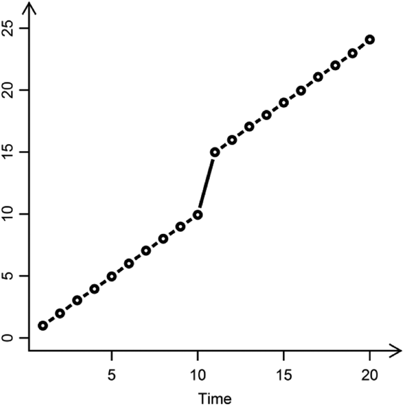
Structure of data with one discontinuity and equal slopes.

Table 4 provides parameter estimates from three alternative models. The parameter estimates are based on ordinary least squares (OLS) regression because the code generates nonindependent data (the ICC is effectively zero). In practice, data collected over time typically contains a high degree of nonindependence and can also contain serial autocorrelation within the Level 1 residuals, so one would use mixed-effects models to avoid bias in standard errors (Bliese & Hanges, 2004; Littell, Milliken, Stroup, & Wolfinger, 1996; Raudenbush and Bryk, 2002; Singer & Willett, 2003). In this example, however, we are not focusing on standard errors, and OLS estimates appropriately illustrate how parameter estimates reflect data with a known structure represented by alternative time-related covariates.

Table 4.

Parameter Estimates From Basic Discontinuous Model.

	Estimate
(Intercept)	0.996
TIME	0.998
TRANS	4.008
RECOV	0.006
(Intercept)	0.996
TIME.A	0.998
TRANS	5.007
RECOV	1.004
(Intercept)	0.996
TIME.R	0.998
TRANS	4.008
RECOV	1.004

The first block of Table 4 presents parameter estimates from standard coding. In this model, the estimate of the intercept (0.996) represents the value of the dependent variable in the referent group (pre-transition) at TIME 0 (the first occasion). The model parameters indicate that (a) a one unit change in TIME is associated with a one unit change in SCORE (0.998), (b) values increase by 4 (4.008) at the transition, and (c) the recovery slope is effectively zero (0.006). The latter two estimates are interpreted relative to TIME. That is, the value for TRANS is 4 rather than 5 (the value generated in the code) because the TRANS estimate reflects change based on the TIME and intercept parameters. Specifically, the generated value of 15 is 4 greater than the expected value of 11 based on the intercept (≈1) plus 10 increases of the TIME parameter (10 × 0.998). RECOV is effectively zero because it is also interpreted relative to TIME, and both TIME and RECOV have the same slope.

The second block of Table 4 reflects parameter estimates when TIME is held at 9 at the transition point in the coding we refer to as TIME.A. Notice in this model that both TRANS and RECOV are interpreted relative to zero. Specifically, TRANS increases by 5 points (5.007) and the recovery slope is 1 (1.004). Finally, the third block represents coding where the TIME vector continues the sequence through the first transition point (TIME.R). Notice that TRANS is interpreted relative to the pre-transition slope (again reflecting 4.008) while RECOV is interpreted relative to zero (1.004).

The coding used in TIME.A is clearly valuable for testing absolute change, and the use of TIME, TIME.A, and TIME.R together provide clear and thorough descriptions of relative and absolute change patterns. It is worth noting that each of the three model specifications fit the data equally well. The residual sum of squares is identical at 19,892 for each model, so the choice of coding alternatives revolves around interpreting model parameters. It is also worth noting that in this example, the inferences drawn from the parameter estimates are (by design) straightforward. In practice, the magnitudes of parameter estimates (and hence their interpretation) can be considerably more ambiguous, thereby making the use of alternative coding approaches helpful in interpreting patterns.

Two Discontinuities

A second extension of the basic discontinuous model we consider is one containing two discontinuities. As noted, Aguinis et al. (2010) used a variant of this model to examine the productivity of journal editors over a period with two discontinuities—the discontinuity in the appointment of the editors’ term and the discontinuity at completing the editorial term. Aguinis et al.’s model used two transition points (what we refer to as TRANS1 and TRANS2) and two slope parameters (what we refer to as RECOV1 and RECOV2). As we illustrate, the alternative coding for time (TIME.A and TIME.R) generalize in a straightforward manner to models with multiple TRANS and RECOV covariates; however, for purposes of illustration, we begin by considering a model containing only time and two transition parameters (TIME, TRANS1, and TRANS2).

Two Transitions

When specifying and interpreting models with two (or more) discontinuities, one includes time-related covariates as a block of dummy codes. Table 5 provides an example with two transition parameters based on code in presented in Appendix A. The code creates data for 15 time periods (TIME: 0-14). The first transition (TRANS1) occurs at the 5th time point, and the second transition (TRANS2) occurs at the 10th time point. The dependent variable, SCORE, increases by 5 points (from 5 to 10) at the first transition point and then decreases from 14 to 5 (a 9-point decrease) at the second transition point. TRANS1 represents a dummy-coded value for the first transition period versus the initial period; TRANS2 represents a dummy-coded value for the second transition versus the initial period. In the generated data, TIME increases by 1 point within each of the three periods. The data structure and the first 15 values of SCORE are presented in Table 5. Figure 2 shows the form of the generated data averaging across time.

Table 5.

Generated Data From Two Transitions.

TIME	TRANS1	TRANS2	SCORE
0	0	0	−0.750
1	0	0	1.873
2	0	0	4.052
3	0	0	5.430
4	0	0	4.535
5	1	0	8.995
6	1	0	13.278
7	1	0	12.164
8	1	0	11.732
9	1	0	14.231
10	0	1	5.976
11	0	1	7.017
12	0	1	6.907
13	0	1	7.697
14	0	1	8.141

Figure 2.

Structure of generated data with two discontinuities and equal slopes.

The first block of Table 6 presents the estimated values. The intercept estimate for the referent group (pre-transition) at TIME 0 is 1 (1.019); the TIME parameter reflects the point increase at each time period (0.994), and the value for the first transition (TRANS1) is 4 (4.026). As with the previous example, the parameter estimate reflects the difference between the referent-based expected value of 6 (≈1.019 + 5 × 0.994) and the generated value of 10. The parameter estimate for the second transition (TRANS2) is –6 (–5.957). The parameter estimate at the second point is also interpreted relative to the pre-transition referent. Specifically, at TIME 10 (Period 11; the point of the second transition), the expected value for SCORE based on the pre-transition referent is 11 (≈1.019 + 10 × 0.994), and the generated value of 5 is 6 points lower than 11.

Table 6.

Parameter Estimates From a Model With Two Transitions.

	Estimate
(Intercept)	1.019
TIME	0.994
TRANS1	4.026
TRANS2	−5.957

The strategy of creating dummy codes and using the initial time as the referent for interpreting parameter estimates can be extended to multiple discontinuities. In all cases, the referent for interpreting parameters is the condition where the time-based covariates are all zero. If data are coded such that zero occurs at a point other than Time 1, the interpretation of the estimates can be adjusted; however, the basic logic remains unchanged. For instance, if we subtract 2 from TIME, the zero point for TIME is now aligned with the third occasion (the pre-transition midpoint). With this change, the intercept estimate is now 3 (3.007), reflecting the value on the third occasion. The TIME, TRANS1, and TRANS2 parameters are unchanged (0.994, 4.026, –5.957, respectively). The expected value at occasion 6 (TRANS1) is still 6 (3.007 + 3 × 0.994), resulting in a TRANS1 parameter estimate of 4.

Multiple Transitions and Multiple Recovery Slopes

As an example of how parameter estimates align to data structure with multiple transitions and multiple slopes, we modify the data generating R code in Appendix A so each value for SCORE initially increases by 1 (1:5), but at the first transition point, it decreases from 10 to 6 (10:6), and at the second transition point, it remains flat at 5 (5:5). The code for data generation and variable coding is presented in Appendix A. The first 15 generated observations are presented in Table 7. Figure 3 shows the form of the data averaging across time.

Table 7.

Generated Data From Two Transitions and Two Recovery Slopes.

TIME	TIME.A	TRANS1	TRANS2	RECOV1	RECOV2	SCORE
0	0	0	0	0	0	−0.750
1	1	0	0	0	0	1.873
2	2	0	0	0	0	4.052
3	3	0	0	0	0	5.430
4	4	0	0	0	0	4.534
5	4	1	0	0	0	8.995
6	4	1	0	1	0	11.278
7	4	1	0	2	0	8.164
8	4	1	0	3	0	5.732
9	4	1	0	4	0	6.231
10	4	0	1	0	0	5.976
11	4	0	1	0	1	6.017
12	4	0	1	0	2	4.907
13	4	0	1	0	3	4.697
14	4	0	1	0	4	4.141

Figure 3.

Structure of generated data with two discontinuities and different slope segments.

We begin by modeling and interpreting the transition parameters without including slope parameters. The first block of Table 8 returns the parameter estimates for TRANS1 and TRANS2. Notice that the estimate for TIME is approximately zero, reflecting the fact that SCORE increases for the first five generated values, decreases for the next five values, and remains flat for the last five values. The estimate of the intercept is 3 (3.019), corresponding to the mean value in the referent group (i.e., 3). The TRANS1 value of 5.026 reflects that the mean after the first transition is 5 points above the referent mean (≈8), and the TRANS2 value of 2.043 indicates that the mean after the second transition is 2 points above the referent (≈5).³

Table 8.

Parameter Estimates From Models With Two Transitions and Two Recovery Slopes.

	Estimate
(Intercept)	3.019
TIME	−0.006
TRANS1	5.026
TRANS2	2.043
(Intercept)	1.018
TIME	0.994
TRANS1	4.039
TRANS2	−5.972
RECOV1	−2.007
RECOV2	−0.994
(Intercept)	1.018
TIME.A	0.994
TRANS1	5.033
TRANS2	−0.005
RECOV1	−1.012
RECOV2	0.000

The second block of Table 8 presents a model with two transitions and three slope segments. Recall that data were generated to increase for the first five observations, decrease for the second five, and remain flat for the last five. We interpret each of the model parameters in turn. First, the intercept value of 1 (1.018) reflects the model-based estimate for the referent group on the first occasion. The parameter estimate for TIME is 0.994, reflecting the 1-point increase in the first five observations. TRANS1 is approximately 4 (4.039), reflecting the difference between the expected value of 6 (1.018 + 5 × 0.994) and the generated value of 10. TRANS2 is –6 (–5.972), reflecting the difference between the expected value of 11 (1.018 + 10 × 0.994) and the generated value of 5. The parameter estimate for RECOV1 is –2 (–2.007) and represents the difference between the observed positive value of 0.994 for the pre-transition slope and the generated negative value of –1 for the post-transition slope. Finally, the RECOV2 parameter estimate is –0.994 and is interpreted relative to the initial pre-transition slope of 0.994. The difference between the two is zero, reflecting the fact that the code generated values with a flat slope after the second transition.

As with less complex models, alternative specifications for TIME provide tests of absolute versus relative change. For instance, the TIME.A coding holding TIME at a constant of 4 across all values following the first transition (see Table 7) produces the parameter estimates in the bottom portion of Table 8. Notice that the parameter estimates for the intercept and the pre-transition period remain unchanged; however, the parameter estimate for the first transition (TRANS1) period now reflects the absolute change of the generated values (≈5). The same is true of the other parameters: The TRANS2 value of approximately zero represents the fact that the last value in the pre-transition period (TIME 4) was generated to be 5 and the first value in the second transition period was also generated to be 5; thus, in absolute terms, there is no change. Estimates of slopes (RECOV1 and RECOV2) based on TIME.A reflect absolute change (roughly –1 for the middle slope period and 0 for the latter slope period). Finally, as with the previous examples, a TIME.R variant holding values at 5 following the first transition provides absolute values for slopes but comparative values for transition parameters. Again, it is worth reiterating that the different specifications of TIME do not impact model fit: In all cases (TIME, TIME.A, TIME.R), the residual sum of squares is 14,840.

Quadratic Change in Pre- and Post-Change Periods

A third extension of the basic discontinuous model we discuss is a variant that includes nonlinear reexpressions of the linear terms in the pre- and post-change periods. In this example, we use data reported in Lang and Bliese (2009) rather than data generated with known parameter values (see Appendix B for details). We also use mixed-effects models (lme in R) to estimate the parameter estimates and standard errors because the data contain a high degree of nonindependence. Specifically, in Stage 1, a null model estimate of the ICC is 0.44, indicating that 44% of the variance can be attributed to differences among individuals.

The data from Lang and Bliese (2009) allow us to illustrate how one would incorporate a smooth quadratic change process into the discontinuous growth model. Lang and Bliese used these data to test substantive questions about how differences in general mental ability predicted (a) performance learning trajectories on a complex task, (b) performance when individuals were confronted with an unexpected change, and (c) performance trajectories post-change. In the research paradigm, it was important to include a nonlinear term because skill acquisition on complex tasks asymptotically decreased over time. Therefore, Lang and Bliese included an additional time-based parameter for quadratic change associated with (a) the pre-transition slope and (b) the recovery slope.

The basic structure of the time-varying covariates is provided in Table 9. Notice the inclusion of squared terms for TIME (TIME.SQ) and for RECOV (RECOV.SQ). In what follows, we illustrate how permutations of the time-varying covariates can be used to model the change processes within Stage 2 (examining fixed-effects associated with time) of the model building process. To facilitate this illustration, we present a series of steps in Table 10 and follow these steps in the analysis of the data. Our reported values are similar but not identical to values reported in Lang and Bliese (2009) because we illustrate parameter estimates using less complex random effects in our models (specifically, we estimate random intercept models without random slopes at this stage). Table 11 provides a detailed analysis of Stage 2 following the steps in Table 10. In Table 11, the parameter estimate is followed by the t value. Standard errors can be calculated by dividing the t value by the parameter estimate.

Table 9.

Data Structure From Lang and Bliese (2009).

Measurement Occasion	TIME	TIME.SQ	TRANS	RECOV	RECOV.SQ	TIME.A	TIME.R
1	0	0	0	0	0	0	0
2	1	1	0	0	0	1	1
3	2	4	0	0	0	2	2
4	3	9	0	0	0	3	3
5	4	16	0	0	0	4	4
6	5	25	0	0	0	5	5
7	6	36	1	0	0	5	6
8	7	49	1	1	1	5	6
9	8	64	1	2	4	5	6
10	9	81	1	3	9	5	6
11	10	100	1	4	16	5	6
12	11	121	1	5	25	5	6

Table 10.

Model Testing Sequence.

Step	Change Variables in the Model	Interpretation
Step 1a	TIME TRANS RECOV	Relative change in transition and recovery
Step 1b	TIME.A TRANS RECOV	Absolute change in transition and recovery
Decision on the basis of Step 1		When relative or absolute change in the transition is nonsubstantial, execute Step 2a. When relative or absolute change in the recovery is nonsubstantial, execute Step 2b. When relative or absolute change in the transition or recovery is substantial or borderline, examine Step 3.
Step 2a	TIME RECOV	Compare to Step 1; when the substantial interpretation of the model does not change, the transition can be omitted.
Step 2b	TIME TRANS	Compare to Step 1; when the substantial interpretation of the model does not change, the recovery slope can be omitted.
Step 3a	TIME TIME.SQ TRANS RECOV RECOV.SQ	Relative change in transition and quadratic change
Step 3b	TIME.A TIME.A.SQ TRANS RECOV RECOV.SQ	Absolute change in transition and quadratic change

Table 11.

Discontinuous Change in the Decision-Making Data With Alternative Specifications of Time.

	Step 1a	Step 1b	Step 2a	Step 2b	Step 3a	Step 3b	Lang & Bliese
Fixed effects
Intercept	−3.69 (−5.84)	−3.69 (−5.84)	−2.16 (−3.65)	−2.49 (−4.04)	−4.73 (−6.83)	−4.73 (−6.83)	−4.73 (−6.83)
TIME	1.81 (14.46)		1.20 (13.42)	1.10 (12.23)	3.37 (7.57)		3.37 (7.57)
TIME.A		1.81 (14.46)				3.37 (7.57)
TIME.SQ					−0.31 (−3.65)
TIME.A.SQ						−0.31 (−3.65)	−0.31 (−3.65)
TRANS	−4.98 (−8.05)	−3.17 (−5.90)	−4.37 (−7.06)		−2.09 (−1.99)	−2.15 (−3.21)	−5.53 (−7.96)
RECOV	−1.22 (−6.88)	0.59 (4.73)		−1.02 (−5.70)	1.00 (1.33)	0.63 (1.42)	−2.74 (−4.35)
RECOV.SQ					0.30 (2.51)	−0.01 (−0.09)	−0.01 (−0.09)
Random effects (variance)
Intercept	46.82	46.82	46.73	46.69	46.85	46.85	46.85
Residual	50.66	50.66	51.82	52.25	50.37	50.37	50.37
Fit indices
−2Log	15,391.81	15,391.81	15,437.00	15,456.48	15,384.69	15,384.69	15,384.69
AIC	15,403.81	15,403.81	15,447.00	15,466.48	15,400.69	15,400.69	15,400.69
BIC	15,438.00	15,438.00	15,475.49	15,494.97	15,446.27	15,446.27	15,446.27

Note: Values in parentheses are t values. Divide the estimates by the t values to get the standard errors. AIC = Akaike Information Criterion; BIC = Bayesian Information Criterion.

Step 1a

Step 1a represents what we define as the basic discontinuous growth model. Performance at the first occasion in the referent condition (pre-change) is –3.69 and increases 1.81 units each time period. Upon encountering the unexpected change, participants decline 4.98 points relative to the predicted value based on the intercept and the TIME parameter. The recovery slope is –1.22, indicating that it is less steep than the pre-transition slope. Both the TRANS and RECOV parameters are significant, indicating significant relative differences.

Step 1b

In Step 1b, TIME.A is substituted for TIME to provide absolute estimates of the TRANS and RECOV parameters. Notice that TRANS changes values, but the sign continues to be negative, returning an estimate of –3.17; in contrast, RECOV changes values and changes sign, returning an estimate of 0.59. It is informative that the recovery has both a significant decline relative to the pre-transition slope (–1.22) and a significant positive slope in absolute terms (0.59). Again, both parameters are significant, but the values based off TIME.A reflect tests of significance for absolute change. As observed in the OLS models, the fit indices for Step 1a and Step 1b show that the two models are identical in terms of –2log likelihood, AIC, and BIC values; however, it is clear that the two alternative specifications of TIME provide different information and together produce a thorough understanding of the nature of the linear changes in performance over the course of the experiment.

Step 2a and 2b

Given that both the TRANS and the RECOV parameters were significant, there would be little value in specifying the simplified models in 2a and 2b (see Table 10); however, for illustrative purposes, we estimate the models in Table 11. Notice that the included parameters are significant, but based on the AIC and BIC indices (where smaller is better), one would conclude that the model specifications in Steps 1a and 1b provide a better fit to the data. In a choice between Models 2a and 2b, it would be reasonable to conclude (based on AIC and BIC) that the model with a step decrease and parallel lines for the pre-transition and recovery slope (Model 2a) fits better than the model without a transition step decrease with different slopes pre- and post-transition (Model 2b).

Step 3a

Step 3a represents a basic quadratic model where the TIME vector and the RECOV vector are squared (TIME.SQ and RECO.SQ, respectively). As in regression models (e.g., Cohen, Cohen, West, & Aiken, 2003), the lower-order terms are influenced by the higher-order terms when interpreting models. That is, the linear terms in the models with squared terms refer to the linear term at a particular point in time and change as a function of the higher-order terms across time (Biesanz, Deeb-Sossa, Papadakis, Bollen, & Curran, 2004). For instance, the linear terms for TIME refer to the linear effect at the origin of time. Therefore, the parameters to examine first are TIME.SQ, TRANS, and RECOV.SQ (TRANS can be interpreted because it has no corresponding higher-order term). Based on the parameter estimates in Step 3a, we conclude that a significant quadratic term exists prior to the transition. The term is negative (–0.31), suggesting a negative accelerating curve consistent with asymptotic decreases in learning. The transition estimate is negative (–2.09) and represents a relative decrease based on an expected value from parameter estimates of the intercept, the linear term, and the quadratic term. The RECOV.SQ term is 0.30, suggesting a positive quadratic term relative to the TIME.SQ term. Notice that the absolute estimate for the recovery quadratic term is near zero (0.30 larger than –0.31)—a difference we formally test in the next model.

Step 3b

Using TIME.A rather than TIME again defines all subsequent parameters in absolute terms. Model results from Step 3b show that the intercept (–4.73) and pre-transition quadratic slope (–0.31) are identical to values in Model 3a. In Model 3b, however, TRANS represents absolute change (–2.15), as does the post-transition quadratic slope (–0.01). Expressing parameter estimates in terms of absolute change is clearly informative in the complex model represented by both linear and quadratic change pre- and post-transition. For instance, one can quickly observe that performance dropped by 2.15 points at the transition. Note also that the post-transition quadratic slope is flat as expected based on the previous model.

Mixing Relative and Absolute Effects

The examples provided in the models in Steps 3a and 3b represent cases where the linear and quadratic terms were both treated as relative versus absolute. That is, TIME was paired with TIME.SQ in the relative model, and TIME.A was paired with TIME.A.SQ in the absolute model. There may be cases, however, where it is helpful to express one aspect of the model in relative terms while expressing another in absolute terms. For instance, the last column of Table 11 (labeled “Lang and Bliese”) shows a model using TIME and TIME.A.SQ. Parameters from the mixed model provide relative terms for TRANS and absolute terms for RECOV.SQ. In this model, the TRANS parameter is –5.53 while the RECOV.SQ parameter is –0.01, as it was in the absolute model in Step 3b. This coding yields a model that incorporates quadratic change but is conceptually similar to the basic discontinuous growth model (Step 1a) with a couple of other advantages.

In the Lang and Bliese coding, the transition is coded relative to the linear rate of skill acquisition that participants showed at the origin of time. The transition consequently denotes the drop in performance controlling for (and thus relative to) participants’ baseline capacity to acquire the task. Subtracting the relative TRANS effect from the linear effect approximately yields the absolute TRANS effect in model Step 3b (3.37 – 5.53 = –2.16) and demonstrates that the two models are equivalent. In a similar vein, the linear reacquisition (RECOV) is coded relative to the rate of skill acquisition at the origin of time (TIME) and consequently denotes participants’ capacity to reacquire the task relative to their skill acquisition in the task. The RECOV effect is negative, indicating that participants were less capable of acquiring the task immediately after the transition than during the pre-transition period. Subtracting the relative RECOV effect from the rate of change at the origin of time therefore yields the absolute rate of change after the transition from Step 3b (3.37 – 2.74 = 0.63), demonstrating model equivalence.

Step 3b (expressing parameters in absolute terms) and the model used by Lang and Bliese complement each other. Specifically, researchers will often be interested in whether a drop in performance occurred at the transition and whether individuals were able to reacquire the task. However, for theoretical reasons, when researchers are interested in understanding differences in trajectories, it is also important to separate the processes that occur as a result of the transition from ordinary skill acquisition processes (and thus examine TRANS and RECOV relative to baseline skill acquisition). Accordingly, we suggest that researchers use these two models to draw inferences on absolute and relative change in discontinuous models.

Limitations of Step 3a Model

In concluding the discussion of models with quadratic processes, it is informative to consider details surrounding the interpretation of the basic Step 3a model expressing relative change in both linear and quadratic terms. Our experience is that this model is less useful than Step 3b and the model used in Lang and Bliese. To understand why, it is important to consider that Step 3a parameters are defined relative to both the linear and quadratic change in the pre-transition period. Thus, the model describes the transition correcting for a hypothetical scenario where skill acquisition continued beyond the transition period, which may not be logical if the task has changed.

The coefficients from the model demonstrate the effect. The predicted value at the end of the pre-change skill acquisition period is ([–4.73] + 3.37 × 5 + [–0.31 × 5²] = 9.1). The predicted value at the first period after the transition is ([–4.73] + 3.37 × 6 + [–0.31 × 6²] = 9.06), reflecting a predicted value for a hypothetical scenario that would have existed if the transition had not occurred. The difference between these two values is –0.05 (9.1 – 9.06 = –0.05) and approximately accounts for the difference in the predicted transition between the Step 3a (relative parameters) and the Step 3b (absolute parameters) models, (–0.04) + (–2.09) ≈ –2.15. What may be counterintuitive is the fact that the relative parameters predict a very small but negative decrease in performance because of the skill acquisition process. Although this negative effect is quite small, it demonstrates a general limitation of the Step 3a model. Specifically, Model 3a generalizes curvilinear change beyond the timeframe on which the original linear mixed-effects model was fit. Conceptually, we consider it problematic that the model generalizes the skill acquisition process beyond the transition point. We also note that the statistical literature has long recognized that linear models including curvilinear change are ill-suited for generalizing beyond the originally fit time period (see Pinheiro & Bates, 2000, pp. 273-275). Accordingly, we caution researchers against using the model in Step 3a and recommend its use only in situations where researchers are confident that a curvilinear polynomial change model is valid beyond the transition time period.⁴

Extending the Example Beyond Stage 2

While our focus has been on Stage 2 modeling of time-related covariates, Stages 3 and 4 are critical aspects of developing and testing growth models that depend on decisions made in Stage 2. Stage 3 examines characteristics of the random effects within the models. One central question addressed in Stage 3 is whether the time-varying fixed effects vary across individuals. Information from Stage 3 is relevant for Stage 4 where one attempts to predict sources of variance. As noted, in terms of substantive research questions related to the Lang and Bliese (2009) example, Stage 3 provides the basis to ask whether individuals significantly vary in terms of (a) the pre-transition trajectory, (b) the degree of change observed at the transition, and (c) the post-transition trajectory.

Stage 3 Slope Variation

Given our focus on Stage 2 and the alternative specifications of TIME, an important question is whether the Stage 3 tests of –2log likelihood differences are similar for models with different specifications of TIME. For instance, we have shown that using TIME.A instead of TIME produces parameter estimates for TRANS and RECOV that reflect absolute instead of relative differences. It may not be clear, however, whether –2log likelihood tests of TRANS and RECOV would be the same with different specifications of TIME.

Table 12 presents results of Stage 3 analyses for a model specified in relative terms with the use of TIME (Model Step 1a in Table 11) versus the results of Stage 3 for a model specified in absolute terms using TIME.A (Model Step 1b in Table 11). Notice that the log likelihood values differ. Both models suggest that individuals significantly differed with respect to the transition (TRANS). That is, regardless of whether the transition is expressed in relative terms (–4.98) or absolute terms (–3.17), one would conclude that participants responded differently to the unexpected change. In contrast, the models suggest different interpretations for recovery (RECOV). The absolute slope of the recovery (0.59) did not significantly vary across individuals while the slope expressed relative to the pre-transition (–1.22) slope did vary. Clearly, the use of TIME versus TIME.A tests different theoretical assumptions with respect to both the transition and the recovery slope. Furthermore, as we discuss in Stage 4, these differences are particularly significant for interpreting RECOV parameters.

Table 12.

Stage 3 –2log Likelihood Tests of Random Effects: Relative Change Versus Absolute Change Model Specifications.

Random Term	Model	df	AIC	BIC	logLik	Test	L.Ratio	p Value
Intercept	1	6	15,403.81	15,438.00	−7,695.90
TIME	2	8	15,390.63	15,436.21	−7,687.31	1 vs 2	17.18	.00
TIME + TRANS	3	11	15,342.24	15,404.92	−7,660.12	2 vs 3	54.39	.00
TIME + TRANS + RECOV	4	15	15,331.75	15,417.22	−7,650.88	3 vs 4	18.49	.00
Intercept	1	6	15,403.81	15,438.00	−7,695.90
TIME.A	2	8	15,406.06	15,451.65	−7,695.03	1 vs 2	1.75	.42
TIME.A + TRANS	3	11	15,330.29	15,392.97	−7,654.15	2 vs 3	81.77	.00
TIME.A + TRANS + RECOV	4	15	15,331.78	15,417.25	−7,650.89	3 vs 4	6.52	.16

Note: AIC = Akaike Information Criterion; BIC = Bayesian Information Criterion; L.Ratio = likelihood ratio.

Finally, note that the TIME parameter also varied in the relative model (likelihood ratio of 17.18) but not in the absolute model (likelihood ratio of 1.75) despite having an identical parameter estimate of 1.81. It would appear that the use of TIME.A provides a more conservative test based on potential slope variability restricted to the pre-transition time (recall values are invariant after the transition). In other words, tests based on TIME (relative coding) may be influenced by post-transition variation.

Stage 4 Parameters

Based on Stage 3 results, we can conclude that individuals significantly differ in terms of the degree of performance decline at the transition and (if conducting tests of relative change) also in terms of the pre-transition slope and post-transition slope. Therefore, in Stage 4 we identify individual characteristics that explain these differences, and for didactic purposes, we explore a predictor of TIME/TIME.A, TRANS, and RECOV using both relative and absolute coding.

For illustrative purposes, we examine participant conscientiousness as a Level 2 predictor. Table 13 provides parameter estimates from two models where participant conscientiousness is used to predict difference in all three time-related covariates. For simplicity, we omit potential quadratic effects and provide estimates based on random intercept models: Models with random slopes have similar parameter values but different standard errors (see Appendix B).

Table 13.

Stage 4 Parameter Estimates With Conscientiousness as a Predictor.

	Value	SE	df	t Value	p Value
Relative coding
(Intercept)	−3.69	0.63	2,018	−5.86	.00
TIME	1.81	0.13	2,018	14.47	.00
TRANS	−4.98	0.62	2,018	−8.05	.00
RECOV	−1.22	0.18	2,018	−6.88	.00
CONSCIEN	−0.45	0.63	182	−0.72	.47
TIME:CONSCIEN	−0.22	0.13	2,018	−1.78	.07
CONSCIEN:TRANS	0.98	0.62	2,018	1.58	.11
CONSCIEN:RECOV	0.29	0.18	2,018	1.63	.10
Absolute coding
(Intercept)	−3.69	0.63	2,018	−5.86	.00
TIME	1.81	0.13	2,018	14.47	.00
TRANS	−3.17	0.54	2,018	−5.90	.00
RECOV	0.59	0.13	2,018	4.73	.00
CONSCIEN	−0.45	0.63	182	−0.72	.47
TIME:CONSCIEN	−0.22	0.13	2,018	−1.78	.07
CONSCIEN:TRANS	0.76	0.54	2,018	1.40	.16
CONSCIEN:RECOV	0.07	0.13	2,018	0.52	.60

The upper model in Table 13 uses TIME and expresses TRANS and RECOV parameters in relative terms. The lower model uses TIME.A and expresses TRANS and RECOV in absolute terms. Both models are identical in terms of overall fit; however, the last two parameter estimates associated with the interactions differ between the two models. The upper model tests whether conscientiousness interacts with the relative change at the transition and with the relative slope during the recovery (parameter estimates values of 0.98 and 0.29, respectively). The lower model tests whether conscientiousness interacts with the absolute change at the transition and with the absolute slope during the recovery (0.76 and 0.07, respectively).

While none of the interactive effects in Table 13 meet conventional criteria for significance, it is nonetheless informative to plot the interactions to facilitate interpreting parameter estimates. Figure 4 presents the form of the interactions for the interactive effects involving conscientiousness. Figure 4a represents plots from relative coding (using TIME); Figure 4b represents plots from absolute coding (using TIME.A). Notice that the absolute and relative forms of the model provide identical predicted values in the plots. Pre-transition, those with high conscientiousness have a less pronounced increase in performance than those with low conscientiousness (both models have parameter estimates of –0.22). Recall from Table 11 (see also Table 13) that the transition parameter estimate for the relative effect was stronger (–4.98) than the estimate for the absolute effect (–3.17); therefore, an interactive effect involving relative change should be greater than an interactive effect involving absolute change, explaining why the parameter estimate is 0.98 in the relative model versus 0.76 in the absolute model.

Figure 4.

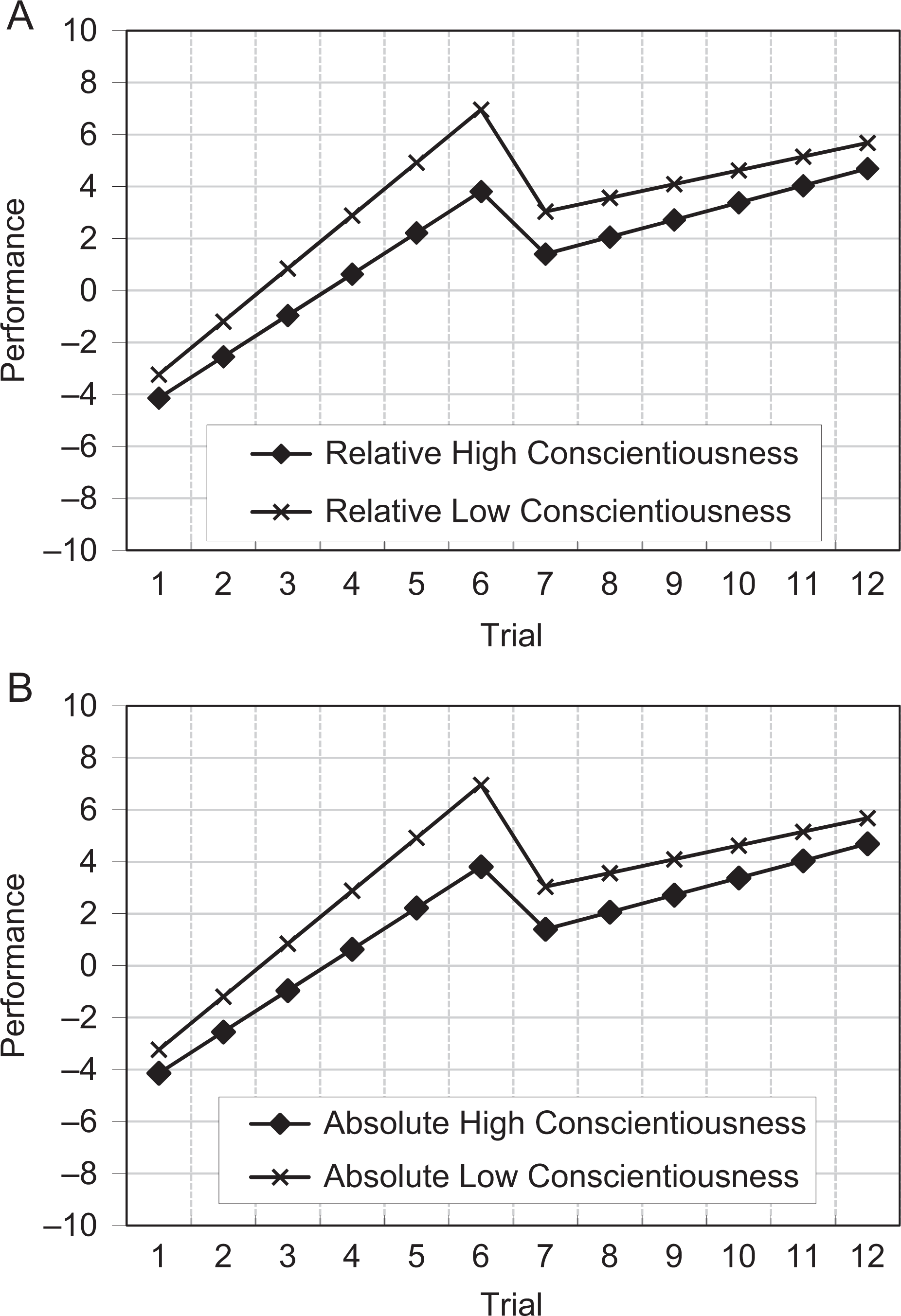
Interaction between conscientiousness and time-based covariates. (a) Relative coding versus (b) absolute coding.

Conceptually, the figures provide an intuitive interpretation of the Conscientiousness × RECOV interaction terms. We begin by interpreting the absolute change parameters in Table 13 based on TIME.A (lower block of parameter estimates). In this model, the parameter estimate tests the interactive effects of the slope lines post-transition. Notice in either Figure 4a or 4b that there is a weak convergence over time between those high and those low in conscientiousness, reflected in the parameter estimate of 0.07. In contrast, in the relative model, the Conscientiousness × RECOV interaction term contrasts the form of the post-transition interaction relative to the form of the pre-transition interaction. Visually, in the pre-transition period, individuals with high and low conscientiousness diverged over time (parameter estimate of –0.22), whereas in the post-transition period, individuals with high and low conscientiousness converged (0.07). The difference between this divergence (–0.22) and convergence (0.07) is 0.29—the parameter estimate for the Conscientiousness × RECOV in relative coding. Thus, while relative versus absolute specifications of time produce the same visual image of an interaction effect, the interpretation fundamentally differs. We elaborate on this point in the discussion.

Discussion

In this article, we have argued that (a) organizational data with numerous repeated measures characterized by one or more discontinuities are common, (b) discontinuous growth models offer considerable potential, and (c) alternative specifications of TIME provide enhanced precision in terms of testing inferences about change. Table 14 provides a summary of the coding alternatives and how the different forms of coding link to tests of absolute versus relative change. What we refer to as the basic discontinuous growth model is specified in the first row, and variants of the basic model that return parameter estimates testing various combinations of absolute versus relative effects are presented in the subsequent rows. Using this table, one can quickly identify the appropriate coding for a variety of models. It is worth noting that while the table presents coding for single transitions and/or single recoveries, the principles detailed in the table generalize to multiple transitions. For instance, TIME, TRANS1, TRANS2, RECOV1, and RECOV2 would return parameters for transition and recovery relative to TIME at each point, whereas TIME.A, TRANS1, TRANS2, RECOV1, and RECOV2 would return parameters in absolute terms at each point.

Table 14.

Coding for Discontinuous Growth Models.

Transition Parameter (TRANS)	Recovery Slope Parameter (RECOV)	Quadratic Recovery Slope (RECOV.SQ)	Time-Related Covariates
Relative to pre-transition	Relative to pre-transition		TIME + TRANS + RECOV
Absolute change	Absolute change		TIME.A + TRANS + RECOV
Relative to pre-transition	Absolute change		TIME.R + TRANS + RECOV
Not estimated	Relative to pre-transition		TIME + RECOV
Not estimated	Absolute slope		TIME.A + RECOV
Relative to pre-transition	Not estimated (equal to pre)		TIME + TRANS
Absolute change	Not estimated (equal to pre)		TIME.A + TRANS
Not estimated	Relative to pre-transition	Relative to pre-transition	TIME + TIME.SQ + RECOV + RECOV.SQ
Not estimated	Absolute slope	Absolute slope	TIME.R + TIME.SQ + RECOV + RECOV.SQ
Relative to pre-transition	Relative to pre-transition	Relative to pre-transition	TIME + TIME.SQ + TRANS + RECOV + RECOV.SQ
Relative to pre-transition	Absolute slope	Absolute slope	TIME.R + TIME.SQ + TRANS + RECOV + RECOV.SQ
Absolute change	Absolute slope	Absolute slope	TIME.A + TIME.SQ + TRANS + RECOV + RECOV.SQ

In the examples motivating Table 14, the data structure was consistent in that transitions occurred at the same time point. In some situations, however, it may not be possible to align data so that the transition occurs at the same time point for each entity. For instance, Singer and Willett (2003) use an example regressing wages on the discontinuity event of receiving a GED for a sample of high school dropouts. In the example, study participants received their GED at different points and had different numbers of measurement occasions prior to receiving GEDs (indeed, not all participants received their GEDs). One can easily imagine other situations (e.g., studies of retirement, changes of leadership in groups, etc.) where potentially discontinuous events occur at different times in a data collection sequence.

Figure 5 illustrates a simple example where transitions do not align across entities. In the figure, the circles experience a transition at Time 10 while the triangles experience a transition at Time 15. While the data structure may make data management more complicated, the interpretation of parameter estimates generalizes from the case where transitions occur at the same point. For instance, the R code in Appendix A generates data matching Figure 5 with 500 entities following the circle pattern and 500 entities following the triangle pattern. The data were generated with a one-point increase each time period, a five-point increase at the transition, and a one-point increase after the transition. Thus, the pattern in the data is similar to the pattern illustrated in Table 3 and which produced the parameter estimates in Table 4 except that in Figure 5, the transition occurs at occasion 15 for half the entities. While not shown, the parameter estimates based off the structure described in Figure 5 will be approximately one, one, four, zero for intercept, TIME, TRANS, and RECOV, respectively, and approximately one, one, five, one when modeled as absolute change (TIME.A). In other words, the parameter estimates from the data structure in Figure 5 (with transitions occurring at different times) will match the parameter estimates in the simpler case presented in Table 3. Interested readers can confirm this using Appendix A code. Our point is that having the transition occur at different points for different entities produces a model that can be interpreted as if the transition points had occurred at the same point for each entity, and thus the taxonomy in Table 14 holds in these cases as well.

Figure 5.

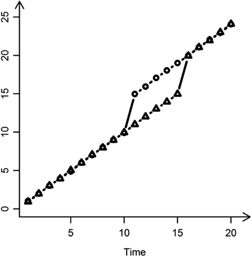
Data where discontinuities occur at different times.

Hypothesis Generation

Throughout the article, we have provided numerous examples of the types of questions that can be examined using discontinuous growth models. Having detailed absolute versus relative coding, we more thoroughly examine how complementary ways of specifying parameters augment researchers’ ability to specify and test hypotheses about complex longitudinal data. Given the richness of the models and the diversity of data to which the models can be applied, it is not possible to provide concrete recommendations that will generalize to all settings. It is, however, possible to illustrate hypothesis generation via several examples. To begin, we review the types of hypotheses that can be generated within the various stages.

Stage 2 (delineating the nature of the change process) can either serve as a step supporting Stage 3 and Stage 4 or provide results testing specific hypotheses. When Stage 2 is used to test hypotheses, two conditions will generally be true: The nature of the change process is unknown, and the change process is assumed to be similar for all Level 2 entities (no interactions). Examples include examinations of editor productivity (Aguinis et al., 2010) and policy changes in education (e.g., Raudenbush, 2009). In all the Stage 2 examples, research questions center on trajectories that are presumably altered by some event. As a rule of thumb, Stage 2-centered research will almost always benefit from testing complementary models that examine both relative and absolute change. Even if theory does not support differentiating between relative and absolute change, the additional knowledge about the change process garnered from examining absolute and relative change is valuable. Interestingly, when the pre-transition period has a significant slope, tests involving absolute change about the transition (i.e., comparing TRANS to zero) will generally be more stringent than tests of relative change (i.e., comparing TRANS to pre-transition based expected values). In contrast, the opposite will often be true of tests of absolute change for the recovery slope (RECOV). That is, it will generally be easier to demonstrate that recovery slopes differ from zero than to show that recovery slopes differ from the pre-recovery slope.

One’s choice of absolute versus relative tests in Stage 2 should also be informed by the nature of the discontinuous event. For instance, in certain circumstances, the event causing the initial slope is removed at the point of discontinuity. Clear examples would be studies of sleep restriction and recovery (e.g., Bliese, Wesensten, & Balkin, 2006; Rupp, Wesensten, Bliese, & Balkin, 2009) where the slope representing performance changes associated with sleep restriction was interrupted by removing sleep restriction. In these cases, one can argue that hypotheses and tests should focus on absolute change. Consider, for example, that a test of relative change surrounding the transition assumes that it is meaningful to extrapolate an existing trajectory driven by sleep restriction to a time at a future point where the event driving the initial trajectory had been removed. In other cases, the discontinuous event may be considered one of numerous factors influencing a trajectory so questions of relative change are more meaningful: One can logically assume that declines in customer satisfaction, for instance, are multifaceted, so examining how a change (a new customer engagement program) is related to relative change in the transition and recovery is meaningful (though they still may be augmented with tests of absolute change).

Stage 3 is routinely used as a building block for Stage 4 but can also potentially serve to support hypotheses that center on homogeneity of responses to the change process. For instance, Stage 3 examinations of cognitive performance trajectories in the pre-recovery transition helped document the existence of reliable individual differences in response to sleep restriction (Bliese et al., 2006; see also Van Dongen, Baynard, Maislin, & Dinges, 2004). As shown in Table 12, absolute versus relative model specifications impact the –2loglikelihood tests that form the basis of Stage 3 tests. Therefore, it is important to consider the meaning of the model parameters when contrasting models.

Stage 4 focuses on identifying interaction effects surrounding Stage 3 variability and represents the most complex situation regarding alternative coding of time. Recall from Table 13 that alternative coding evokes different contrasts and thus produces different parameter estimates for the post-change interaction terms (see CONSCIEN × TRANS and CONSCIEN × RECOV). As a general rule, it will be valuable to examine both relative and absolute effects associated with interactions involving TRANS; however, decisions about whether to focus on absolute versus relative change with respect to interactions associated with the RECOV term need to be carefully considered. For many analytic questions, interaction tests involving absolute differences will be of interest. For instance, in a randomized trial where Level 2 units are randomly assigned to two or more conditions, pre-transition slopes would presumably be equal between groups. In this situation, tests of absolute differences in slope trajectories post-intervention would be most informative. That is, following an intervention, one would be interested in the slope trajectories of the different groups irrespective of any existing pre-transition data.

In other situations, however, one might formally want to test relative change. For instance, if one had a theoretical reason to expect that a pre-transition pattern (divergent pattern) would be reversed post-transition (convergent pattern), the appropriate test would be based on relative coding. In some ways, the use of relative coding with respect to interactions with the recovery term is most appropriate when theory can be framed in terms analogous to those used to describe three-way interactions. In other words, the theoretical proposition would be framed as a two-way interaction between time and a construct of interest pre-transition being significantly different than the form of the two-way interaction post-transition. If the theoretical arguments cannot be articulated in a way analogous to a three-way interaction, then relative coding is not likely to be appropriate.

In sum, effective and compelling hypothesis generation requires specific knowledge of what is being tested within each stage using alternative specifications of time. The examples have shown that different stages of the process lead to different types of hypotheses, and within these stages, alternative specifications of time have further implications for developing and testing hypotheses.

Summary and Conclusions

While the technical details surrounding the specification of discontinuous growth models are a straightforward extension of growth models, the interpretation of parameter estimates from discontinuous growth models is not always straightforward. By detailing how alternative ways of specifying time leads to alternative interpretations of the parameter estimates, we have attempted to clarify and refine how discontinuous growth models can be used to test a variety of theoretical assumptions. More specifically, we have shown that simple changes to the time vector can be used to generate parameter estimates that test for absolute differences rather than relative differences. The ability to test for absolute change enhances researchers’ ability to understand the nature of the change process and that it also allows more precision when specifying and testing hypotheses. We anticipate that the models we have described will be applied with increasing frequency to a wide range of repeated measures data and that our ability to develop and refine theory will, in part, be contingent upon correctly interpreting model parameters.

Footnotes

Appendix A

Appendix B

#######################

# Read csv datafile (available from authors)

#######################

tankdat<-read.csv(file.choose())

names(tankdat)

stage1<-lme(SCORE∼1, random=∼1|ID, tankdat)

VarCorr(stage1)

46.16066/(46.16066+58.59416) # ICC estimate

###############################

# Create TIME-related variables

###############################

tankdat$TIME.SQ<-tankdat$TIME⁁2

tankdat$TRANS<-ifelse(tankdat$TIME<6,0,1)

tankdat$RECOV<-tankdat$TIME-6; tankdat$RECOV[tankdat$RECOV<0]<-0

tankdat$RECOV.SQ<-tankdat$RECOV⁁2

tankdat$TIME.A<-ifelse(tankdat$TIME<5, tankdat$TIME,5)

tankdat$TIME.R<-ifelse(tankdat$TIME<6, tankdat$TIME,6)

#Table 9

tankdat[1:12, c(“TIME”,”TIME.SQ”,”TRANS”,”RECOV”,”RECOV.SQ”,”TIME.A”,

“TIME.R”)]

#Table 11

step1a<-lme(SCORE∼TIME+TRANS+RECOV, random=∼1|ID, tankdat,

control=lmeControl(opt=“optim”))

round(summary(step1a)$tTable, dig=2)

VarCorr(step1a)

-2*logLik(step1a); AIC(step1a); BIC(step1a)

step1b<-update(step1a, SCORE∼TIME.A+TRANS+RECOV)

round(summary(step1b)$tTable, dig=2)

VarCorr(step1b)

-2*logLik(step1b); AIC(step1b); BIC(step1b)

step2a<-update(step1a, SCORE∼TIME+TRANS)

round(summary(step2a)$tTable, dig=2)

VarCorr(step2a)

-2*logLik(step2a); AIC(step2a); BIC(step2a)

step2b<-update(step1a, SCORE∼TIME+RECOV)

round(summary(step2b)$tTable, dig=2)

VarCorr(step2b)

-2*logLik(step2b); AIC(step2b); BIC(step2b)

step3a<-update(step1a, SCORE∼TIME+TIME.SQ+TRANS+RECOV+RECOV.SQ)

round(summary(step3a)$tTable, dig=2)

VarCorr(step3a)

-2*logLik(step3a); AIC(step3a); BIC(step3a)

tankdat$TIME.A.SQ<-tankdat$TIME.A⁁2 #create at TIME.A squared term

step3b<-update(step1a, SCORE∼TIME.A+TIME.A.SQ+TRANS+RECOV+RECOV.SQ)

round(summary(step3b)$tTable, dig=2)

VarCorr(step3b)

-2*logLik(step3b); AIC(step3b); BIC(step3b)

lbcoding<-update(step1a, SCORE∼TIME+TIME.A.SQ+TRANS+RECOV+RECOV.SQ)

round(summary(lbcoding)$tTable, dig=2)

VarCorr(lbcoding)

-2*logLik(lbcoding); AIC(lbcoding); BIC(lbcoding)

# Table 12

stage3b2<-update(step1a, random=∼TIME|ID)

stage3b3<-update(step1a, random=∼TIME+TRANS|ID)

stage3b4<-update(step1a, random=∼TIME+TRANS+RECOV|ID)

anova(step1a, stage3b2, stage3b3, stage3b4)

stage3b2<-update(step1b, random=∼TIME.A|ID)

stage3b3<-update(step1b, random=∼TIME.A+TRANS|ID)

stage3b4<-update(step1b, random=∼TIME.A+TRANS+RECOV|ID)

anova(step1b, stage3b2, stage3b3, stage3b4)

# Table 14

stage4a<-lme(SCORE∼TIME+TRANS+RECOV+CONSC+TIME: CONSC+TRANS: CONSC+RECOV: CONSC,

random=∼1|ID, tankdat, control=lmeControl(opt=“optim”))

summary(stage4a)$tTable

-2*logLik(stage4a); AIC(stage4a); BIC(stage4a)

stage4b<-lme(SCORE∼TIME.A+TRANS+RECOV+CONSC+

TIME.A: CONSC+TRANS: CONSC+RECOV: CONSC,

random=∼1|ID, tankdat, control=lmeControl(opt=“optim”))

summary(stage4b)$tTable

-2*logLik(stage4b); AIC(stage4b); BIC(stage4b)

# Alternative Table 14 with random effects

stage4a<-lme(SCORE∼TIME+TRANS+RECOV+CONSC+

TIME: CONSC+TRANS: CONSC+RECOV: CONSC,

random=∼TIME+TRANS+RECOV|ID, tankdat, control=lmeControl(opt=“optim”))

summary(stage4a)$tTable

stage4b<-lme(SCORE∼TIME.A+TRANS+RECOV+CONSC+

TIME.A: CONSC+TRANS: CONSC+RECOV: CONSC,

random=∼TIME.A+TRANS+RECOV|ID, tankdat,

control=lmeControl(opt=“optim”))

summary(stage4b)$tTable

Declaration of Conflicting Interests

The author(s) declared no potential conflicts of interest with respect to the research, authorship, and/or publication of this article.

Funding

The author(s) received no financial support for the research, authorship, and/or publication of this article.

Notes

References

Aguinis

de Bruin

G. P.

Cunningham

Hall

N. L.

Culpepper

S. A.

Gottfredson

R. K.

(2010). What does not kill you (sometimes) makes you stronger: Productivity fluctuations of journal editors. Academy of Management Learning & Education, 9, 683–695.

Barkema

H. G.

Schijven

(2008). Toward unlocking the full potential of acquisitions: The role of organizational restructuring. Academy of Management Journal, 51, 696–722.

Bhaskar-Shrinivas

Harrison

D. A.

Shaffer

M. A.

Luk

D. M.

(2005). Input-based and time-based models of international adjustment: Meta-analytic evidence and theoretical extensions. Academy of Management Journal, 48, 257–281.

Biesanz

J. C.

Deeb-Sossa

Papadakis

A. A.

Bollen

K. A.

Curran

P. J.

(2004). The role of coding time in estimating and interpreting growth curve models. Psychological Methods, 9, 30–52.

Bliese

P. D.

Hanges

P. J.

(2004). Being both too liberal and too conservative: The perils of treating grouped data as though it is independent. Organizational Research Methods, 7, 400–417.

Bliese

P. D.

McGurk

Thomas

J. L.

Balkin

T. J.

Wesensten

(2007). Discontinuous growth modeling of adaptation to sleep setting changes: Individual differences and age. Aviation, Space, and Environmental Medicine, 78, 485–492.

Bliese

P. D.

Ployhart

R. E.

(2002). Growth modeling using random coefficient models: Model building, testing, and illustrations. Organizational Research Methods, 5, 362–387.

Bliese

P. D.

Wesensten

Balkin

T. J.

(2006). Age and individual variability in performance during sleep restriction. Journal of Sleep Research, 15, 376–385.

Blumenthal

Tavenner

(2010). The “meaningful use” regulation of electronic health records. New England Journal of Medicine, 363, 501–504. doi:10.1056/NEJMp1006114

10.

Boswell

W. R.

Shipp

A. J.

Payne

S. C.

Culbertson

S. S.

(2009). Changes in newcomer job satisfaction over time: examining the pattern of honeymoons and hangovers. Journal of Applied Psychology, 94, 844–858.

11.

Canato

Ravasi

Phillips

(2013). Coerced practice implementation in cases of low cultural fit: Cultural change and practice adaptation during the implementation of Six Sigma at 3 PM. Academy of Management Journal, 56, 1724–1753.

12.

Chen

(2005). Newcomer adaptation in teams: Multilevel antecedents and outcomes. Academy of Management Journal, 48, 101–116.

13.

Cohen

West

S. G.

Aiken

L. S.

(2003). Applied multiple regression/correlation analysis for the behavioral sciences (3rd ed.). Mahwah, NJ: Lawrence Erlbaum Associates.

14.

Cudeck

Klebe

K. J.

(2002). Multiphase mixed-effects models for repeated measures data. Psychological Methods, 7, 41–63.

15.

Greenberg

(2006). Losing sleep over organizational injustice: Attenuating insomniac reactions to underpayment inequity with supervisory training in interactional justice. Journal of Applied Psychology, 91, 58–69.

16.

Halbesleben

J. R. B.

Wheeler

A. R.

Paustian-Underdahl

S. C.

(2013). The impact of furloughs on emotional exhaustion, self-rated performance, and recovery experiences. Journal of Applied Psychology, 98, 492–503.

17.

Hausman

J. A.

(1978). Specification tests in econometrics. Econometrica, 46, 1251–1271.

18.

Hernández-Lloreta

M. V.

Colmenares

Martínez-Arias

(2004). Application of piecewise hierarchical linear growth modeling to the study of continuity in behavioral development of baboons (Papio hamadryas). Journal of Comparative Psychology, 118, 316–324.

19.

Hox

J. J.

(2002). Multilevel analysis: Techniques and applications. Mahwah, NJ: Lawrence Erlbaum Associates.

20.

Johnson

M. D.

Hollenbeck

J. R.

Humphrey

S. E.

Ilgen

D. R.

Jundt

Meyer

C. J.

(2006). Cutthroat cooperation: Asymmetrical adaptation to changes in team reward structures. Academy of Management Journal, 49, 103–119.

21.

Kim

Ployhart

R. E.

, (2014). The effects of staffing and training on firm productivity and profit growth before, during, and after the great recession. Journal of Applied Psychology, 99, 361–389.

22.

Kozlowski

S. W. J.

Chao

G. T.

Chang

C.-H.

Fernandez

(2016). Team dynamics: Using “big data” to advance the science of team effectiveness. In Tonidandel

King

Cortina

(Eds.), Big data at work: The data science revolution and organizational psychology. New York, NY: Routledge Academic.

23.

Kramer

Chung

(2015). Work demands, family demands, and BMI in dual-earners families: A 16-year longitudinal study. Journal of Applied Psychology, 100, 1632–1640.

24.

Lang

J. W. B.

Bliese

P. D.

(2009). General mental ability and two types of adaptation to unforeseen change: Applying discontinuous growth models to the task-change paradigm. Journal of Applied Psychology, 92, 411–428.

25.

Lang

J. W. B.

Kersting

(2007). Regular feedback from student ratings of instruction: Do college teachers improve their ratings in the long run? Instructional Science, 35, 187–205.

26.

LePine

J. A.

(2005). Adaptation of teams in response to unforeseen change: Effects of goal difficulty and team composition in terms of cognitive ability and goal orientation. Journal of Applied Psychology, 90, 1153–1167.

27.

LePine

J. A.

Colquitt

J. A.

Erez

(2000). Adaptability to changing task contexts: Effects of general cognitive ability, conscientiousness, and openness to experience. Personnel Psychology, 53, 563–593.

28.

Littell

R. C.

Milliken

G. A.

Stroup

W. W.

Wolfinger

R. D.

(1996). SAS system for mixed models. Cary, NC: SAS Institute Inc.

29.

Lucas

R. E.

Clark

A. E.

Georgellis

Diener

(2004). Unemployment alters the set point of life satisfaction. Psychological Science, 15, 8–13.

30.

Marquis

Huang

(2010). Acquisitions as exaptation: The legacy of founding institutions in the U.S. commercial banking industry. Academy of Management Journal, 53, 1441–1473.

31.

Mundlak

(1978). On the pooling of time series and cross section data. Econometrica, 46, 69–85. doi:10.2307/1913646

32.

Parker

S. K.

(2003). Longitudinal effects of lean production on employee outcomes and the mediating role of work characteristics. Journal of Applied Psychology, 88, 620–634.

33.

Pinheiro

J. C.

Bates

D. M.

(2000). Mixed-effects models in S and S-PLUS. New York, NY: Springer-Verlag.

34.

R Core Team. (2014). R: A language and environment for statistical computing. Vienna, Austria: R Foundation for Statistical Computing. Retrieved from http://www.r-project.org

35.

Raudenbush

S. W.

(2009). Adaptive centering with random effects: An alternative to the fixed effects model for studying time-varying treatments in school settings. Education, 4, 468–491.

36.

Raudenbush

S. W.

Bryk

A. S.

(2002). Hierarchical linear models: Applications and data analysis methods. Newbury Park, CA: Sage.

37.

Rupp

T. L.

Wesensten

N. J.

Bliese

P. D.

Balkin

T. J.

(2009). Banking sleep: Realization of benefits during subsequent sleep restriction and recovery. Sleep, 32, 311–321.

38.

Singer

J. D.

Willett

J. B.

(2003). Applied longitudinal data analysis: Modeling change and event occurrence. New York, NY: Oxford University Press.

39.

Van Dongen

H. P. A.

Baynard

M. D.

Maislin

Dinges

D. F.

(2004). Systematic inter-individual differences in neurobehavioral impairment from sleep loss: Evidence of trait-like differential vulnerability. Sleep, 27, 423–433.

40.

Wang

(2007). Profiling retirees in the retirement transition and adjustment process: Examining the longitudinal change patterns of retirees’ psychological well-being. Journal of Applied Psychology, 92, 455–474.

Measurement Occasion	TIME	TRANS	RECOV	TIME.A	TIME.R
1	0	0	0	0	0
2	1	0	0	1	1
3	2	0	0	2	2
4	3	0	0	3	3
5	4	0	0	4	4
6	5	1	0	4	5
7	6	1	1	4	5
8	7	1	2	4	5
9	8	1	3	4	5
10	9	1	4	4	5

Measurement Occasion	TIME	TIME.SQ	TRANS	RECOV	RECOV.SQ	TIME.A	TIME.R
1	0	0	0	0	0	0	0
2	1	1	0	0	0	1	1
3	2	4	0	0	0	2	2
4	3	9	0	0	0	3	3
5	4	16	0	0	0	4	4
6	5	25	0	0	0	5	5
7	6	36	1	0	0	5	6
8	7	49	1	1	1	5	6
9	8	64	1	2	4	5	6
10	9	81	1	3	9	5	6
11	10	100	1	4	16	5	6
12	11	121	1	5	25	5	6

Measurement Occasion	TIME	TRANS	RECOV	TIME.A	TIME.R
1	0	0	0	0	0
2	1	0	0	1	1
3	2	0	0	2	2
4	3	0	0	3	3
5	4	0	0	4	4
6	5	1	0	4	5
7	6	1	1	4	5
8	7	1	2	4	5
9	8	1	3	4	5
10	9	1	4	4	5

Measurement Occasion	TIME	TIME.SQ	TRANS	RECOV	RECOV.SQ	TIME.A	TIME.R
1	0	0	0	0	0	0	0
2	1	1	0	0	0	1	1
3	2	4	0	0	0	2	2
4	3	9	0	0	0	3	3
5	4	16	0	0	0	4	4
6	5	25	0	0	0	5	5
7	6	36	1	0	0	5	6
8	7	49	1	1	1	5	6
9	8	64	1	2	4	5	6
10	9	81	1	3	9	5	6
11	10	100	1	4	16	5	6
12	11	121	1	5	25	5	6

Measurement Occasion	TIME	TRANS	RECOV	TIME.A	TIME.R
1	0	0	0	0	0
2	1	0	0	1	1
3	2	0	0	2	2
4	3	0	0	3	3
5	4	0	0	4	4
6	5	1	0	4	5
7	6	1	1	4	5
8	7	1	2	4	5
9	8	1	3	4	5
10	9	1	4	4	5

Measurement Occasion	TIME	TIME.SQ	TRANS	RECOV	RECOV.SQ	TIME.A	TIME.R
1	0	0	0	0	0	0	0
2	1	1	0	0	0	1	1
3	2	4	0	0	0	2	2
4	3	9	0	0	0	3	3
5	4	16	0	0	0	4	4
6	5	25	0	0	0	5	5
7	6	36	1	0	0	5	6
8	7	49	1	1	1	5	6
9	8	64	1	2	4	5	6
10	9	81	1	3	9	5	6
11	10	100	1	4	16	5	6
12	11	121	1	5	25	5	6