
Abstract
Multiple imputation (MI) is one of the principled methods for dealing with missing data. In addition, multilevel models have become a standard tool for analyzing the nested data structures that result when lower level units (e.g., employees) are nested within higher level collectives (e.g., work groups). When applying MI to multilevel data, it is important that the imputation model takes the multilevel structure into account. In the present paper, based on theoretical arguments and computer simulations, we provide guidance using MI in the context of several classes of multilevel models, including models with random intercepts, random slopes, cross-level interactions (CLIs), and missing data in categorical and group-level variables. Our findings suggest that, oftentimes, several approaches to MI provide an effective treatment of missing data in multilevel research. Yet we also note that the current implementations of MI still have room for improvement when handling missing data in explanatory variables in models with random slopes and CLIs. We identify areas for future research and provide recommendations for research practice along with a number of step-by-step examples for the statistical software R.
Keywords
Multilevel models have become one of the standard tools for analyzing clustered empirical data. Such data are often found in organizational psychology, for example, when employees are nested within work groups or enterprises, or in longitudinal studies when measurement occasions are nested within persons. In addition, empirical data are often incomplete, for example, when some participants fail to answer all of the items on a questionnaire. Several authors have advocated the use of modern missing data techniques such as multiple imputation (MI) rather than traditional approaches such as listwise deletion (LD; Allison, 2001; Enders, 2010; Little & Rubin, 2002; Newman, 2014; Schafer & Graham, 2002). One central requirement of MI is that the imputation model must be at least as general as the model of interest in order to preserve its key features. In multilevel data, it is important that the imputation model takes the multilevel structure into account (e.g., Andridge, 2011; Drechsler, 2015). However, depending on the research question, the multilevel structure may manifest itself in the analysis model in a number of ways (e.g., random intercepts and slopes, relations between variables within and between groups), leading to a multitude of possible multilevel analysis models, each directed at different research questions (e.g., Aguinis & Culpepper, 2015; Snijders & Bosker, 2012).
The motivation behind the present paper is twofold. First, we offer simulation results regarding the performance of MI when the substantive analysis model belongs to one of several types of multilevel models. Second, we provide an introduction to and recommendations for MI of multilevel data directed toward readers who are not yet familiar with the often technical literature on MI. Our article is divided into four sections. In the first section, we focus on the multilevel random intercept model and discuss imputation procedures that are suitable for application in such models. In the second section, we focus on the random coefficients model and the specific challenges that arise when working with random slopes and cross-level interactions (CLIs). In the third section, we briefly discuss missing data in categorical and group-level variables. In each section, we present results from simulation studies in which we used different MI procedures as well as full-information maximum likelihood (FIML). Finally, in the last section, we provide recommendations for how to handle missing data for different types of multilevel models. We conclude with a discussion of our findings and possible topics for future research.
Missing Data and Multiple Imputation
The basic idea of MI is to replace missing values by forming an “informed guess” that is based on the observed data and a statistical model (the imputation model). Multiple imputation generates several (M) replacements for the missing data by drawing repeatedly from the posterior predictive distribution of the missing data, given the observed data and the parameters of the imputation model. The M data sets completed in this manner are then analyzed separately, yielding M sets of parameter estimates. To obtain final estimates and inferences, these results are pooled using the rules described in Rubin (1987; see also Enders, 2010).
The use of MI in most (but not all) implementations is predicated on the assumption that the data are missing at random (MAR). The definition of MAR, according to Rubin (1976), assumes that a hypothetical complete data set can be divided into observed and unobserved parts,
Two aspects make MI a particularly attractive method for dealing with missing data. First, MI recognizes the uncertainty that is due to missing data by generating multiple (as opposed to single) replacements for each missing value, and by drawing the parameters of the imputation model from Bayesian posterior distributions, given the currently imputed data and a set of prior beliefs. Second, because the imputation phase is separated from the analysis phase, MI is able to make full use of the data by including variables in the imputation model that are either predictive of missingness, thus improving the plausibility that MAR holds, or related to the variables of interest, thus improving the power of its predictions (Collins, Schafer, & Kam, 2001).
Multiple Imputation for Multilevel Models
A crucial point in the application of MI to multilevel data is that the imputation model not only includes all relevant variables, but also that it “matches” the model of interest (i.e., the substantive analysis model; see Meng, 1994; Schafer, 2003). In other words, the imputation model must capture the relevant aspects of the analysis model, making the imputation model at least as general as (or more general than) the analysis model. If the imputation model is more restrictive than the analysis model, then imputations are generated under a simplified set of assumptions, and the results of subsequent analyses may be misleading. For example, consider the case in which the model of interest is a multilevel random intercept model (Snijders & Bosker, 2012) in which an individual-level outcome Y is regressed on an individual-level explanatory variable X

where
Two aspects of the model in Equation 1 are worth noting, and both must be accommodated during MI in order for subsequent analyses to yield proper results. First, the model accounts for the clustered structure of the data by including random effects for each group (Snijders & Bosker, 2012). Therefore, the imputation model must also take the clustered structure into account. Failing to do so, for example, by using single-level MI, might lead to biased parameter estimates and might distort statistical decision making (e.g., Andridge, 2011; Enders, Mistler, & Keller, 2016; Lüdtke, Robitzsch, & Grund, 2017; Taljaard, Donner, & Klar, 2008). Second, the model differentiates between the effects of X at the individual and the group level (i.e., for
Joint Modeling and the Fully Conditional Specification of MI
The procedures available for multilevel MI can be roughly divided into two broad paradigms: the joint modeling approach (JM) and the fully conditional specification of MI (FCS). Both approaches offer the necessary tools for dealing with multilevel missing data. Here, we consider the JM approach implemented in the
Joint modeling (JM)
In the JM approach, a single model is specified for all variables with missing data, and imputations are simultaneously generated from this model for all variables with missing data. For individual-level variables, the joint model reads

where
The design matrices,

where the random effects
The FCS approach
In contrast to the JM approach, the FCS approach imputes missing data separately for each variable with missing data, conditioning on some or all of the other variables in the data set. To address multivariate patterns of missing data, the FCS algorithm iterates back and forth between different target variables. Again, consider the analysis model in Equation 1. For missing data in X and Y, an appropriate FCS approach may generate imputations on the basis of the following two univariate models

The FCS approach iterates between these equations, generating imputations for each missing variable in turn. If both variables are affected by missing data, then the group means are updated at each iteration of the sampling algorithm on the basis of the most recent imputations for X and Y (passive imputation; see below). Similar to JM, unsystematic differences between groups in X and Y are captured by the inclusion of random effects,
Summary
Summing up, there are two points worth noting. First, both the JM and the FCS approach allow for different relations between variables to be estimated at the individual and the group level. Second, the two approaches differ in the way in which they accomplish this task. In the JM, the group level is represented by random effects, whereas the FCS approach relies on the observed group means. However, even though the general approach is different, it has been argued that the two approaches imply similar covariance structures at the individual and the group level and can be used interchangeably (e.g., Carpenter & Kenward, 2013, p. 220; Lüdtke et al., 2017; Mistler, 2015; however, see also Resche-Rigon & White, 2016). Therefore, we expected the two procedures to yield approximately the same, unbiased parameter estimates, making both suitable for MI in quite general applications of the multilevel random intercept model.
Model-Based Treatment using FIML
As an alternative to MI, it is often possible to use model-based procedures such as FIML to treat missing data (for an introduction, see Enders, 2010). FIML is often considered to be very user-friendly because missing data are handled directly during the estimation of the analysis model without requiring any additional steps to be taken by the user (e.g., Allison, 2012; Graham, 2009). Currently, the most popular and versatile implementation of FIML for multilevel models is available in the statistical software Mplus (L. K. Muthén & Muthén, 2012). FIML estimates the parameters of the analysis model directly from the incomplete data set by maximizing the observed-data likelihood. As a result, the use of FIML to treat missing data is closely tied to the analysis model (Schafer & Graham, 2002). In the traditional multilevel model (e.g., Equation 1), the observed-data likelihood includes only the dependent variable in the analysis (e.g., Y), and distributional assumptions are imposed only on that variable. For that reason, FIML initially deals with missing data only in the dependent variable, whereas cases with missing data in explanatory variables are often discarded (see also Hox, van Buuren, & Jolani, 2016). To treat missing data in explanatory variables (e.g., X), the model must be extended in such a way that the likelihood function will incorporate all variables with missing data, thus imposing additional distributional assumptions on the data. In Mplus, this is typically achieved by specifying a set of latent variables for the explanatory variables with missing data (for an illustration, see Enders, 2010).
Although it may not be immediately obvious, this strategy can have negative side-effects in multilevel modeling because of the way in which Mplus estimates multilevel models with latent variables. For example, consider the model in Equation 1 with missing values in X and Y. To estimate this model, Mplus uses a decomposition approach similar to the JM, in which the two variables are decomposed into (latent) individual- and group-level components, each of which is assumed to follow a multivariate normal distribution (Rabe-Hesketh, Skrondal, & Zheng, 2012). However, in doing so, Mplus adopts a different analysis model in which the group-level effects of X on Y are represented by latent variables instead of observed group means (i.e.,
Study 1: Random Intercept Models
Next, we present findings from a computer simulation study in which we compared the performance of different MI procedures in the context of multilevel random intercept models. In addition to the JM and the FCS approach, we also investigated single-level MI, which ignores the multilevel structure altogether, LD, and FIML as discussed above. The main question was which procedures would preserve the relevant features of the substantive analysis model. Here, we provide only a brief sketch of the study’s design. For interested readers, we provide further details in Appendix A.
The substantive analysis model was the random intercept model in Equation 1, and the data were generated from this model. The parameters of the data-generating model were chosen in such a way that they would imply a given value for the intraclass correlations (ICCs) of X and Y. Missing data were generated on Y or X in either a random fashion (MCAR) or conditional on the other variable (MAR). A summary of the simulation conditions is provided in Table 1. We varied the number of groups (k = 50, 100, 200, 500), the number of individuals within each group (n = 5, 10), the ICCs of X and Y (
Simulation Conditions for the Data-Generating Model and the Generation of Missing Values
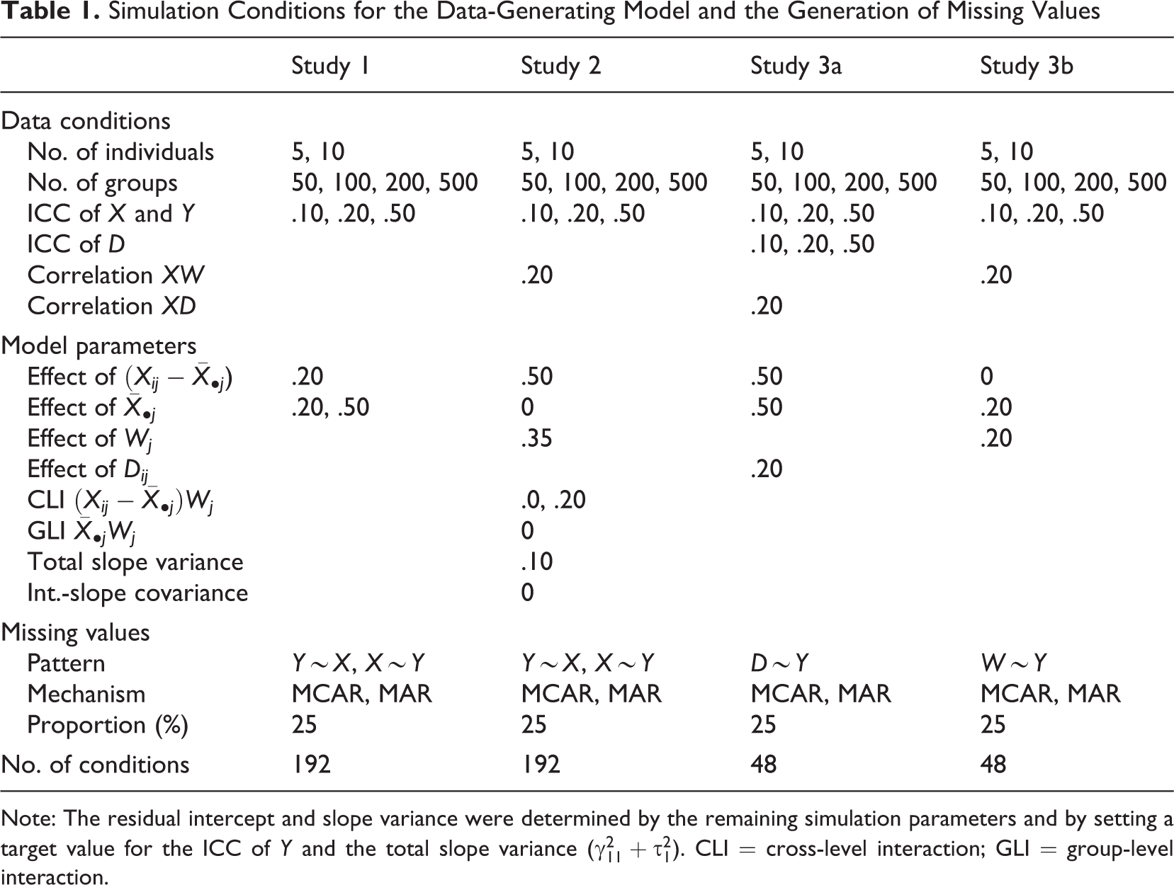
Note: The residual intercept and slope variance were determined by the remaining simulation parameters and by setting a target value for the ICC of Y and the total slope variance (
LD
single-level FCS, ignoring the multilevel structure (FCS-SL)
multilevel FCS with separate within- and between-group effects (Equation 4; FCS-ML)
multilevel JM (Equation 2; JM)
FIML
The parameters of interest were the ICC of Y, estimated from an empty model, and the regression coefficients within and between groups,
Results
Our findings are summarized in Table 2 and Figure 1. The complete collection of results for the parameters of interest is provided in the supplemental online materials. Consistent with our expectations, single-level MI (FCS-SL) reduced the ICC of Y when Y was partially missing. In such a case, the between-group regression coefficient was biased downwards, and the within-group regression coefficient was biased upwards to different extents as determined by the true magnitude of the ICCs of X and Y. With missing values in X, FCS-SL either over- or understated the true size of the regression coefficients, depending on the ICCs. As shown in Figure 1, this bias did not decrease in larger samples. The results from the two appropriate MI procedures (FCS-ML and JM) were similar to one another. Both procedures had a slight tendency to overestimate the ICC of Y and to underestimate the between-group coefficient in smaller samples (i.e.,
Bias (in %), RMSE, and Coverage of the 95% Confidence Interval for the ICC of Y and the Within- and Between-Group Regression Coefficients in Study 1 (Small Groups, n = 5).
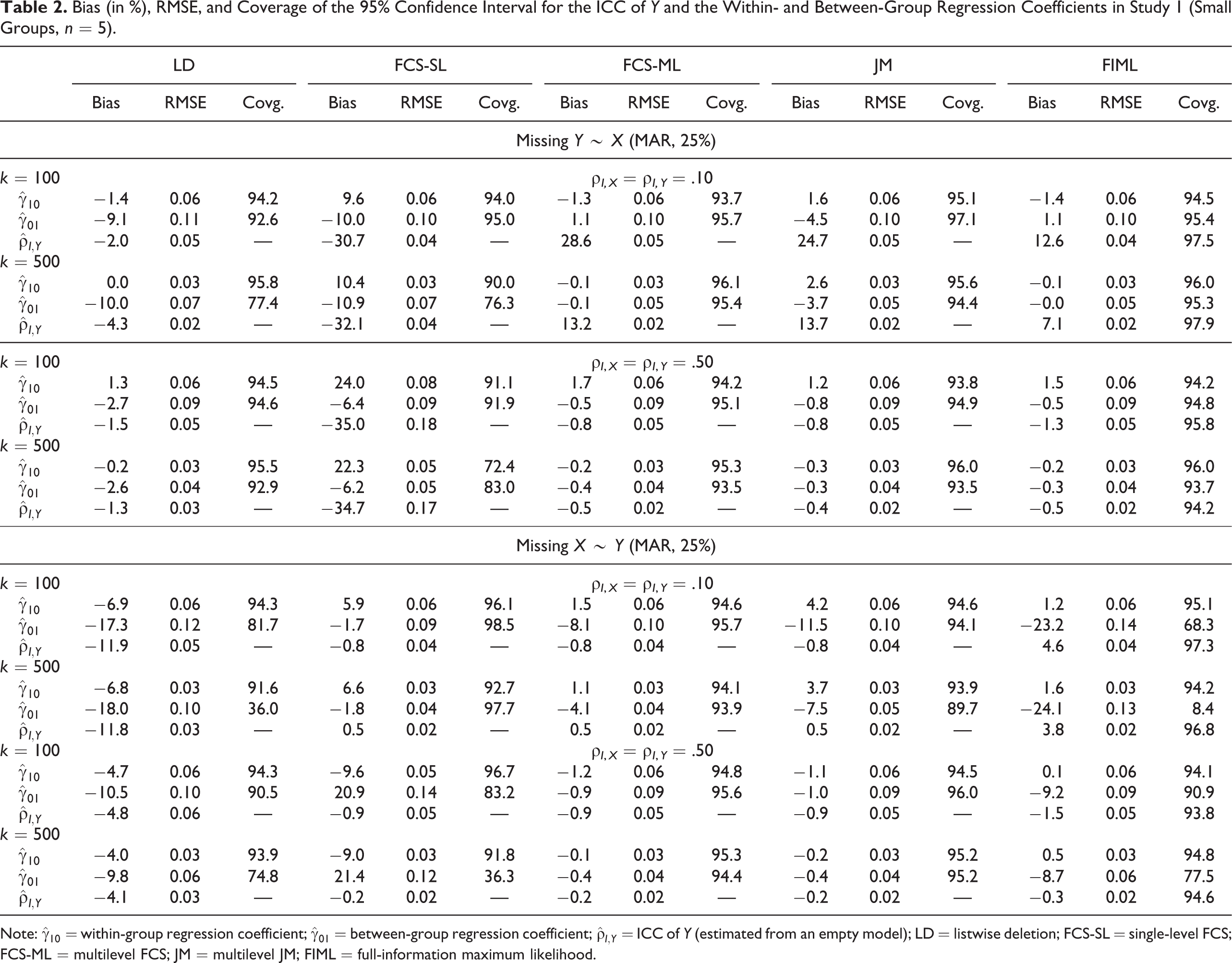
Note:

Estimated bias for the between-group regression coefficient of X (γ01) and the ICC of Y (ρI,Y) in Study 1 for different numbers of individuals (n) and groups (k), moderate ICCs (ρI,X = ρI,Y = .20), and different missing data mechanisms (MAR; Y ∼ X and X ∼ Y). LD = listwise deletion; FCS-SL = single-level FCS; FCS-ML = multilevel FCS; JM = multilevel JM; FIML = full-information maximum likelihood.
The coverage of the 95% confidence interval was acceptable in all conditions for FCS-ML and in all but the most extreme conditions under JM. However, owing to persistent bias, the coverage rates under FCS-SL frequently dropped below 90% in larger samples (i.e., above k = 200, n = 10 or k = 500, n = 5). Coverage rates for FIML were acceptable with missing Y, but dropped below 90% with missing X; those for LD were acceptable under MCAR but unacceptable under MAR. Finally, the RMSE tended to be lowest under FCS-ML and JM as well as under FIML with missing Y. By contrast, the RMSE for the parameters of interest tended to be larger under FCS-SL as well as under LD and FIML with missing X, indicating that these procedures were altogether less accurate and efficient. For example, the average RMSE for the between-group regression coefficient was
Random Slopes and Cross-Level Interactions
Beyond the scope of random intercept models, those engaged in organizational research often seek to understand how the effects of various quantities differ across higher level organizational units. Multilevel models with random slopes allow (a) individual-level effects to vary across groups and (b) for the inclusion of group-level explanatory variables to explain that variability (i.e., CLIs). Recently, Aguinis & Culpepper (2015) stated that random slopes and CLIs were “at the heart of […] any theory that considers outcomes to be a result of combined influences emanating from different levels of analysis,” adding that “the extent to which we understand the presence of cross-level interactions is an indication of theoretical progress” (p. 156).
Consider a multilevel random coefficients model (Snijders & Bosker, 2012) in which an individual-level outcome Y is regressed on an individual-level variable X and a group-level variable W. In addition to the random intercept, we allow the individual-level slope to vary across groups, and we include a CLI to account for some of that variation

where u1j denotes the random slope associated with
Two aspects of the model in Equation 5 are worth noting. First, the slope of the regression of Y on X is assumed to vary across groups. Incorporating the variability in the slope in the imputation model is particularly important if the slope variance itself is of interest, because ignoring the slope variance may lead one to underestimate it in subsequent analyses. Second, the CLI denotes the degree to which the effect of
Accommodating Random Slopes and CLIs
In contrast to applications in the multilevel random intercept model, performing MI is not straightforward when the model of interest includes random slopes and CLIs, particularly when the explanatory variables contain missing data (e.g., Enders et al., 2016; Gottfredson, Sterba, & Jackson, 2016; Grund, Lüdtke, & Robitzsch, 2016a). For example, consider the model of interest in Equation 5. In order for an imputation model to be consistent with this model of interest, it has to acknowledge the fact that the relation between X and Y is assumed to vary both systematically as a function of W (i.e., due to the interaction effects) and unsystematically (i.e., due to random slopes). However, the presence of such terms implies a complex joint distribution for the dependent and explanatory variables which is difficult to emulate in conventional software for multilevel MI (e.g., Kim, Sugar, & Belin, 2015). More advanced methods for accommodating the model of interest when generating imputations are currently being developed, but these are not yet available in standard software for multilevel MI (for further details, see the Discussion section). For this reason, we focus on the procedures that are available in standard software for multilevel MI, which often provide options for accommodating random slopes and CLIs, albeit to different (and arguably imperfect) extents.
Joint modeling (JM)
As mentioned earlier, modeling the joint distribution of the dependent and explanatory variables in a general manner is not a straightforward endeavor if the model of interest includes random slopes or interaction effects. For this reason, we used

where
The FCS approach
To address missing data in multilevel models with random slopes, it has been recommended that researchers specify conditional models that include varying slopes between pairs of variables (Enders et al., 2016). In addition, product terms involving W can be introduced to accommodate the CLI. If both random slopes and product terms are included, the two conditional models become
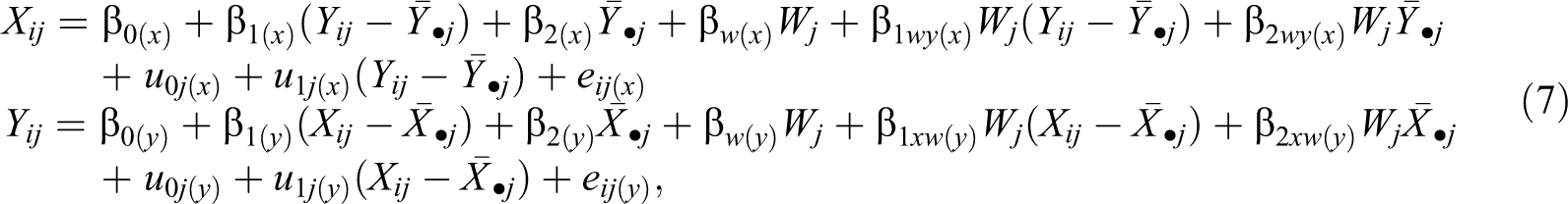
where
There are two aspects worth noting. The first is related to the way in which random slopes are handled in the conditional models. The imputation model for missing values in Y is identical to the analysis model. Thus, imputing Y should be straightforward. However, previous research has shown that missing values in the explanatory variable X pose a much greater challenge because “reversing” the random slope model may produce biased estimates of the regression coefficients and the slope variance in the analysis model (Gottfredson et al., 2016; Grund et al., 2016a; see also Enders et al., 2016). This is not entirely surprising because the analysis model (Equation 5) and the imputation model for missing X (Equation 7, first line) make different statements about the varying relation between X and Y. In other words, although replacing
The second aspect is related to the presence of nonlinear effects (i.e., interaction effects) in the conditional models. At each iteration of the FCS algorithm, the product terms
FIML
Similar to MI, analyzing the incomplete data with FIML can be difficult if the model of interest includes random slopes and CLIs. As before, we focus on FIML estimation in the statistical software Mplus. If missing data occur only on Y, estimating the model of interest in Mplus is straightforward because the observed-data likelihood can be evaluated directly on the basis of the incomplete data. However, if missing values occur on X, it is currently not possible to include X in the analysis model in Mplus without dropping cases with missing X from the analysis (for a discussion, see also Shin & Raudenbush, 2010).
Summary
In contrast to applications in the multilevel random intercept model, missing data pose a greater challenge when the model of interest includes random slopes. Multilevel MI can be expected to provide proper results when only the dependent variable Y contains missing data. However, if the explanatory variable with a random slope, X, contains missing data, conducting MI is not straightforward. Specifically, the “reversed” imputation model for missing X contains only a proxy for the relation of interest, and accommodating product terms (i.e., CLIs and group-level interactions) is still an open area of research (see the Discussion section). As a result, neither JM nor FCS was expected to provide perfect results.
Study 2: Random Slope Models
In this section, we present findings from a simulation study in which we compared different MI procedures in the context of multilevel models with random slopes and CLIs. The model of interest was the random coefficients model presented in Equation 5, and the data were also generated from this model (see Appendix A). The parameters of the data-generating model were chosen in such a way as to imply a given value for the ICCs of X and Y and a given “total” variance for the random slope (i.e., LD single-level FCS, ignoring the multilevel structure and product terms (FCS-SL) multilevel FCS, ignoring random slopes but including passive imputation of product terms (FCS-CLI/no RS) multilevel FCS including random slopes and passive imputation of product terms (Equation 7; FCS-CLI/RS) FIML
The FIML estimation was conducted in Mplus as described above. Because FIML could not be used to estimate the model in conditions with missing X, we included FIML only for conditions with missing Y. The parameters of interest were the within-group regression coefficient of X (
Results
Our main findings are summarized in Table 3 and Figure 2. In presenting our results, we focus on the MI procedures because FIML could be applied only in conditions with missing Y, and the estimates were approximately unbiased in these conditions. For the remaining procedures, the difference between cases with missing data in Y and X was substantial, and sample size continued to play an important role. When only the dependent variable Y was incomplete, FCS-CLI/RS provided approximately unbiased estimates for the parameters of interest, with bias present for the slope variance (
Bias (in %), RMSE, and Coverage of the 95% Confidence Interval for the Within-Group Regression Coefficient of X, the Between-Group Regression Coefficient of W, and the CLI of X with W in Study 2 (Small Groups, n = 5).
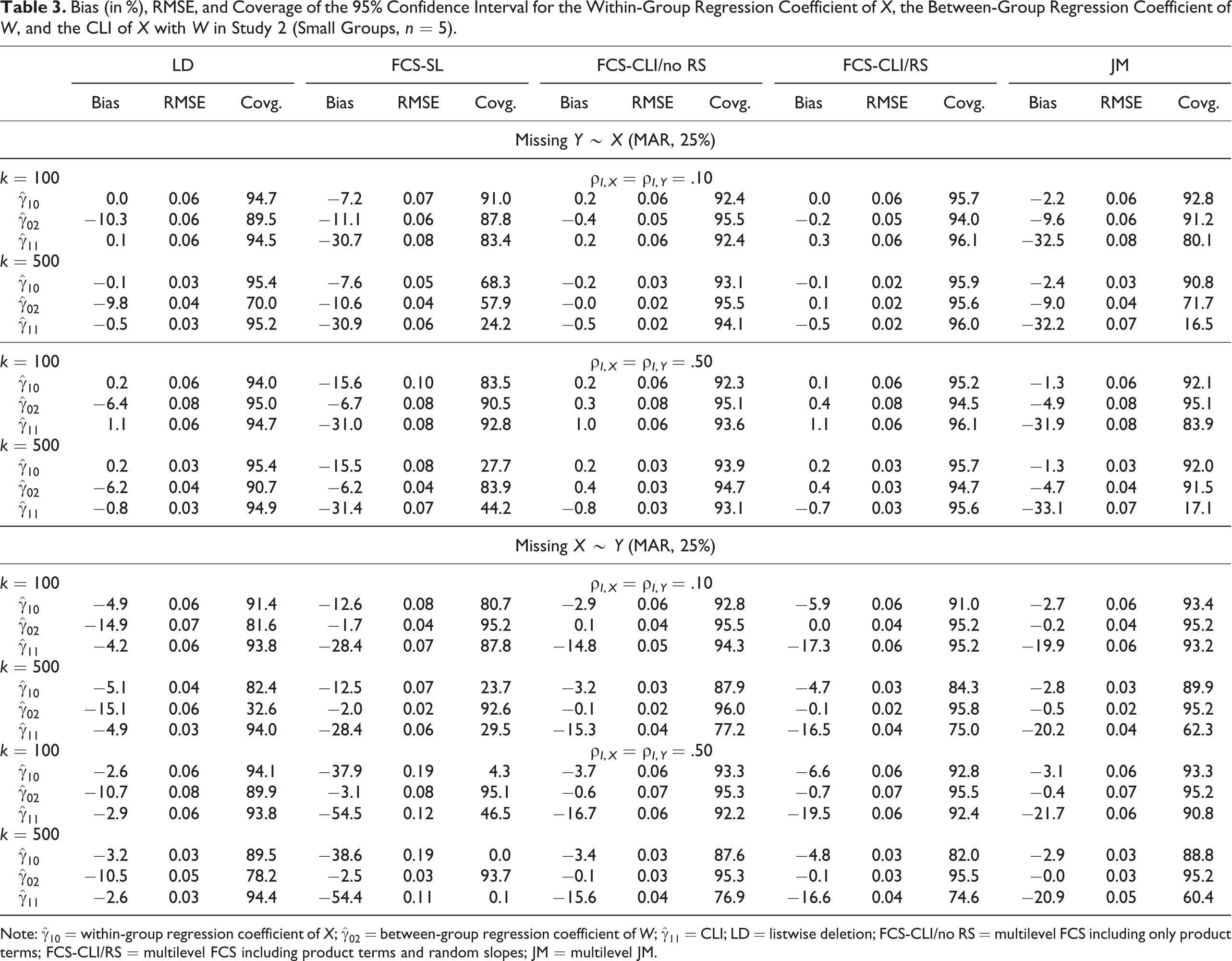
Note:
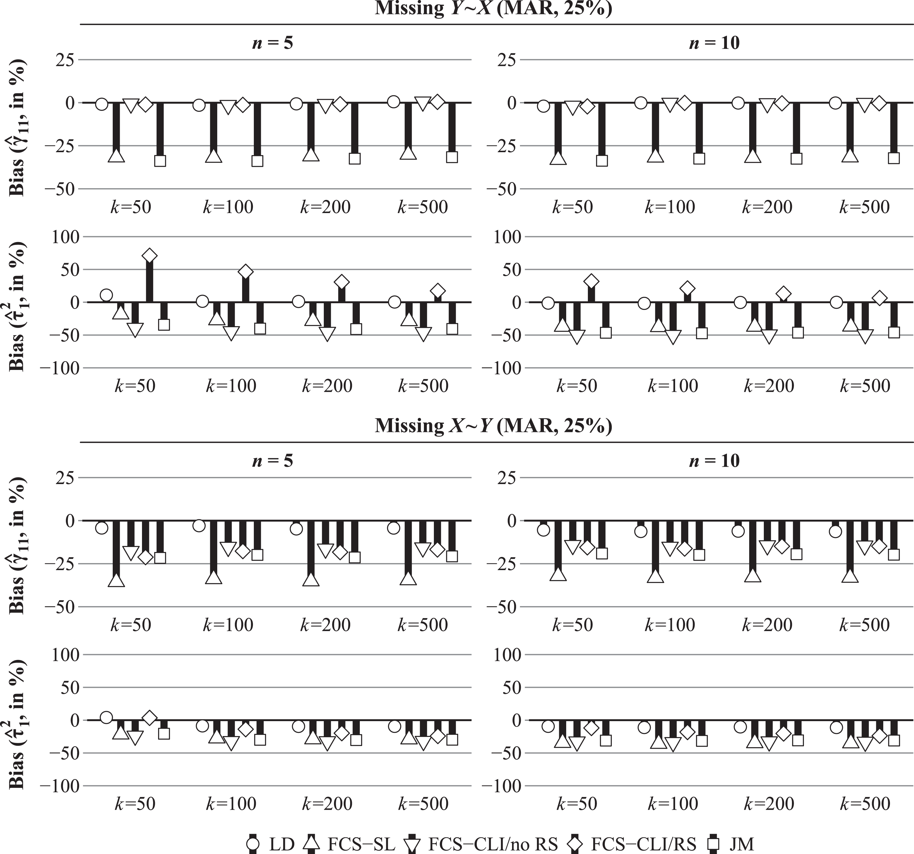
Estimated bias for the CLI (γ11) and the slope variance (
In these cases, both FCS-CLI/no RS and JM also provided approximately unbiased estimates of the regression coefficients (see also Enders et al., 2016; Grund et al., 2016a). Finally, LD provided approximately unbiased estimates of the slope variance, but the estimates of the regression coefficient for W (
When missing values occurred in the explanatory variable X, no procedure provided unbiased estimates of the CLI and the slope variance (see Table 3 and Figure 2). Even when the product terms and random slopes were included in the model (FCS-CLI/RS), multilevel MI provided only biased estimates of the CLI and the slope variance. Ignoring the slope variance (FCS-CLI/no RS) led to slightly better estimates of the regression coefficients but increased the bias in the slope variance. Ignoring both the interaction effects and the random slopes (JM) led to further bias in the CLI but was otherwise comparable to FCS-CLI/no RS. On the other hand, single-level MI (FCS-SL) led to strongly biased estimates of both the main and interaction effects as well as the slope variance. It is interesting that LD provided the least biased estimates of the CLI and the slope variance in conditions with small groups even under MAR. On the other hand, LD introduced bias into the other estimates, particularly the main effect of W when the data were MAR. In conditions with no CLI (
The coverage of the 95% confidence interval and the RMSE were closely related to the bias in the parameter estimates. For FCS-CLI/RS, the coverage was close to the nominal value of 95% for most parameters, but the coverage of the regression coefficient of
Taken together, our results indicate that the FCS approach provides reliable estimates for the parameters of interest when missing values are restricted to Y and still reasonable (though imperfect) estimates with missing values on X. Even though some parameter estimates obtained from FCS were biased, they had better statistical properties overall than those of the competing methods. Ignoring the slope variance sometimes reduced bias in the regression coefficients but resulted in confidence intervals for these coefficients that were too narrow. LD provided the least biased estimates of the slope variance and the CLI but introduced bias in other parameters and tended to be slightly less efficient than MI.
Categorical and Group-Level Missing Data
In the previous two simulation studies, the models of interest were simplified in two ways: (a) the data were always continuous, thus not accounting for missing categorical data, and (b) data were missing only at the individual level, thus not accounting for missing data in group-level variables. Therefore, we conducted two smaller simulation studies that addressed these issues separately.
Study 3a: Missing Categorical Data
Turning back to the random intercept model, researchers are often interested in estimating the differences between groups of participants by including categorical variables in the model of interest, be it to control for group differences (e.g., due to gender, education, etc.) or to assess the effectiveness of interventions (e.g., treatment vs. control group). Especially in the former case, categorical variables may contain missing data. Here, we briefly discuss two procedures for multilevel MI—one using JM, one using FCS—that address missing data in multilevel categorical variables. We also discuss FIML estimation, and we evaluate their performance in a simulation study.
Here, the model of interest is a multilevel random intercept model with two explanatory variables at the individual level, one continuous and one binary

where D is a dummy-coded binary variable that takes on values for each individual i in group j. This model was also used to generate the data (see Appendix A). To ensure that D had a multilevel structure, we simulated a latent background variable
Joint modeling (JM)
Quite general procedures that use the JM approach are available for categorical data (e.g., Goldstein, Carpenter, Kenward, & Levin, 2009). These procedures have been implemented recently in the

where
The FCS approach
Imputations for D may also be generated by directly conditioning on X and Y using FCS. Similar to the joint model, imputations may be generated from a generalized linear mixed-effects model (e.g., with a probit or logit link function)

where
FIML
As an alternative to MI, the model can also be estimated directly by applying FIML. However, because Mplus assumes that the variables in the multilevel model are multivariate normal, it was not straightforward to include D as a multilevel categorical variable. Instead, we treated D as a multilevel continuous normal variable to estimate the model with FIML.
Results
Our main findings are summarized in Table 4. We restricted our reporting to the overall effects of X (
Bias (in %), RMSE, and Coverage of the 95% Confidence Interval for the Overall Regression Coefficients in Study 3a (Missing D ∼ Y, MAR, 25%).

Note:
Study 3b: Group-Level Missing Data
The ideal case in which missing data occur only on the lowest level of multilevel data sets (i.e., on the level of individuals) rarely holds in practice. Moreover, data that are missing at the group level can be particularly cumbersome because they can force researchers to discard complete records at lower levels of the data. For example, consider a study in which employees were asked to rate the frequency of benevolent behavior engaged in by supervisors, and supervisors were asked the same question about their employees. If both variables were to be used as explanatory variables in some model of interest, missing data in supervisor ratings would lead one to discard employees’ ratings as well, resulting in a severe loss of information. Surprisingly, the methodological literature has focused so far on ad hoc procedures, for example, separate imputation of individual- and group-level variables (Gibson & Olejnik, 2003) or “flat file” imputation using single-level MI (Cheung, 2007; for an overview, see Hox et al., 2016; van Buuren, 2011). However, recent advances in statistical software have greatly improved our ability to treat group-level missing data. Here, we briefly discuss two procedures—one using JM, one using FCS—that can be used to impute missing data at the group level.
Here, the model of interest was a multilevel random intercept model with explanatory variables at the individual (e.g., employee ratings) and the group level (e.g., supervisor ratings)

Furthermore, we assumed that W was partially missing. The critical point in this model is that W is measured at the group level; that is, it does not vary across individuals in the same group. Thus, information located at the group level, including the information provided by individual-level variables, may be used to predict missing scores in W. For comparison, we also included LD and single-level FCS.
Joint modeling (JM)
Computationally, the imputation of missing data at the group level is not much different from imputation at the individual level. Specifically, imputations for group-level missing data can be obtained by conditioning on observed group-level variables and on the between-group components of individual-level variables by employing the same general paradigm that is already employed for multilevel MI (for details, see Carpenter & Kenward, 2013; Goldstein et al., 2009). Similar to before, the joint model for the three variables of interest can be written as

where
The FCS approach
Instead of conditioning on the random effects of individual-level variables as in the JM approach, group-level variables can be imputed by applying an FCS approach based on the observed group means of these variables. Specifically, for missing values in W, missing data may be imputed by using the linear regression

where
FIML
Missing values in W can also be addressed using FIML. Because W is directly measured at the group-level, missing data in W can be addressed simply by specifying W as a latent variable in Mplus.
Results
Our main findings are summarized in Table 5. We restricted our reporting to the group-level effects of X (
Bias (in %), RMSE, and Coverage of the 95% Confidence Interval for the Group-Level Regression Coefficients in Study 3b (Missing W ∼ Y, MAR, 25%).
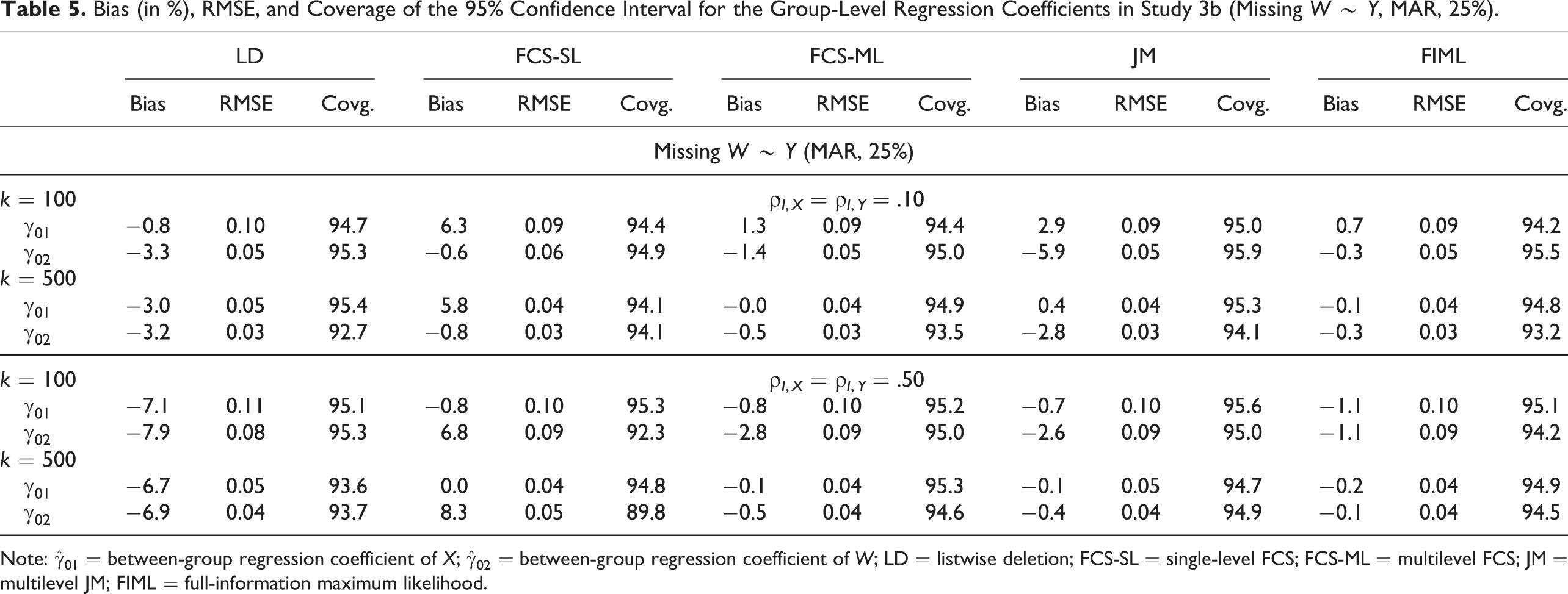
Note:
Recommendations for Practice
There exist several approaches to the treatment of missing data in multilevel designs. As a result, researchers are faced with a multitude of options, several but not all of which may be suitable for a given task. In order to guide researchers in picking a suitable procedure, we provide a detailed list of recommendations in Table 6. This table covers different applications of multilevel models, including applications with random intercepts, random slopes, different variable types, and interaction effects. For each application, we distinguish between a general case with arbitrary patterns of missing data and a number of cases with missing data on specific variables (e.g., categorical and group-level variables). For each case, we list the recommended and not-recommended procedures as well as the likely consequences of choosing the latter.
Finally, we list statistical software that implements one or more of the recommended procedures, and we provide reference to one of the step-by-step examples in Appendix B, which illustrate the use of multilevel MI for each application in the statistical software R (for a general introduction to multilevel MI, see Enders et al., 2016; Grund et al., 2016b).
Recommended Missing Data Treatments and Software for Different Types of Multilevel Analysis Models Recommended Missing Data Treatments and Software for Different Types of Multilevel Analysis Models
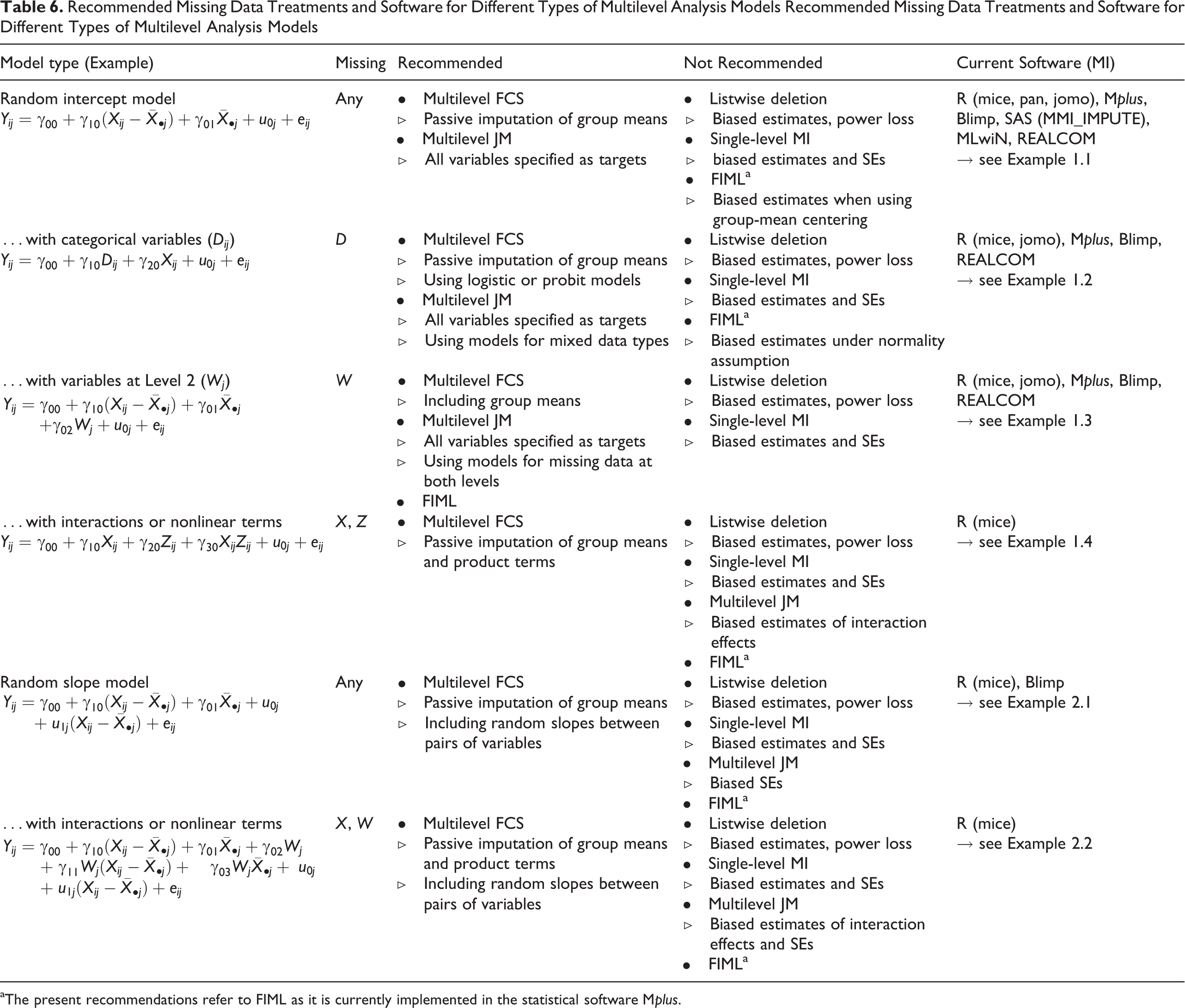
aThe present recommendations refer to FIML as it is currently implemented in the statistical software Mplus.
For applications in the multilevel random intercept model, multilevel MI—using either JM or FCS—provides an effective and general method for dealing with missing data. Procedures for multilevel JM, for example, are implemented in the software packages
Apart from the procedure selected for the treatment of missing data, the performance of MI also depends on a few general factors. For example, researchers should try to include auxiliary variables in the imputation model, that is, variables that are related to either the occurrence of missing data or the variables with missing data themselves (e.g., Collins et al., 2001; Graham, 2009; Schafer & Graham, 2002). When more information can be included from auxiliary variables, then missing values can be inferred from the observed data with greater accuracy (for a discussion about the use of auxiliary variables under FIML, see Enders, 2008; Graham, 2003). In addition, the quality of estimates and inferences obtained from MI can often be improved by generating a larger number of imputations (Bodner, 2008; Graham, Olchowski, & Gilreath, 2007). In our experience, generating 20 imputations is sufficient for most applications in which the primary goal is to estimate the model parameters, but as many as 100 or more imputations can be useful if the analyses involve testing more elaborate statistical hypotheses (Bodner, 2008; see also Grund et al., 2016b).
Discussion
In the present article, we outlined several procedures for MI of multilevel missing data, each intended to accommodate typical research questions in organizational psychology and other areas in the social sciences. Through several smaller simulation studies, we tried to provide a broad overview of multilevel MI. We demonstrated that the current implementations of multilevel MI are able to accommodate quite general research questions and multilevel designs. For example, several procedures for multilevel MI, using either the JM or the FCS approach, were suitable in the broad context of random intercept models. In such a context, missing data can be treated fairly accurately and in a very general manner even when missing data occur at different levels of the sample or in categorical and continuous variables simultaneously.
However, we also pointed out applications in which the current implementations of multilevel MI do not correctly accommodate the model of interest. Specifically, it is still challenging to implement multilevel MI for multilevel models with random slopes or interaction effects when the explanatory variables contain missing data (see also Kim et al., 2015). Even though multilevel FCS appears to be slightly more flexible than multilevel JM in accommodating the substantive model, both approaches ultimately contain limitations due to the ways in which they are currently implemented in statistical software. To alleviate this problem, it has been recommended that the substantive analysis model be taken into account when conducting MI, thus ensuring that imputations are generated in a manner consistent with the model of interest (Bartlett, Seaman, White, & Carpenter, 2015). With this procedure, Bartlett et al. (2015) demonstrated that the bias associated with nonlinear and interaction effects in single-level regression models can be greatly reduced (see also Goldstein, Carpenter, & Browne, 2014). Unfortunately, this approach is currently not available in standard software for multilevel MI.
As an alternative to MI, multilevel models can be estimated directly from the incomplete data by applying model-based procedures such as FIML (e.g., in Mplus). Even though current implementations of FIML are still quite general and easy to use, it can be challenging to estimate multilevel models with missing values in explanatory variables, for example, when the model of interest uses observed group means to incorporate group-level effects or it includes categorical variables, random slopes, or interaction effects (see also Shin & Raudenbush, 2010). The challenges of FIML are ultimately similar to those of MI, and similar proposals have been made with respect to how one might overcome these challenges. For example, Stubbendick & Ibrahim (2003) proposed a factorization approach to FIML estimation of multilevel models with missing data in explanatory variables (see also Wu, 2010). Unfortunately, this approach is also currently not available in standard software. As an alternative, the model-based treatment of missing data can be implemented in a Bayesian analysis approach (Erler et al., 2016; see also Goldstein et al., 2014; Zhang & Wang, 2016). However, the Bayesian approach requires specialized software for Bayesian analyses such as WinBUGS (Lunn, Thomas, Best, & Spiegelhalter, 2000) or JAGS (Plummer, 2016), and such software can be challenging to use in practice (e.g., syntax-based model specification, selection of priors and starting values). Our own experiences indicate that these procedures can provide unbiased estimates with good coverage properties even in multilevel models with random slopes and CLIs. For interested readers, we provide an example of a model-based procedure in the supplemental online materials. This example includes a multilevel model with random slopes and cross- and group-level interactions with missing data in explanatory variables (i.e., the conditions simulated in Study 2). The model syntax for the JAGS software is provided. However, before they can be widely adopted, we recommend that these procedures be subjected to further research and implemented in standard software. Additional software packages that implement FIML for multilevel models are xxM (Mehta, 2013) and Latent GOLD (Vermunt & Magidson, 2013).
Despite limitations in complex multilevel analyses, multilevel MI provides a more reliable and efficient approach to the treatment of missing data in comparison with simpler methods (e.g., single-level MI). As an alternative, it has been suggested that the multilevel structure might be expressed by including dummy-indicator variables in a single-level imputation model (Drechsler, 2015). Although this strategy substantially increases the complexity of the imputation model when the model of interest includes random slopes or interaction effects, it may be interesting to investigate its performance more thoroughly under such conditions (see also Andridge, 2011; Enders et al., 2016). In the context of multilevel models with random slopes, it has also been recommended that single-level MI be performed separately within each group (Graham, 2009). However, this strategy has been shown to be inefficient (i.e., low power) and should be avoided (Taljaard et al., 2008)
Every simulation study has its limitations, and owing to their smaller frame, the simulation studies presented here are no exception. In each study, we focused on varying the sample sizes rather than creating a diverse pattern of possible effects and effect sizes. However, this came at the price of choosing constant values for many of the population parameters. Therefore, the results should not be generalized to arbitrary patterns of effects. On the other hand, it is nearly impossible to address the diversity of possible research designs in a single study. Future studies should investigate the performance of multilevel MI in more specialized applications, including settings with very small samples at the individual level (e.g., dyadic data) or the group level (e.g., research in large organizations), a larger variety of patterns of effects and missing data mechanisms (see Newman, 2009), low ICCs, or a large number of continuous and categorical variables (see Vermunt, 2003; Vermunt, van Ginkel, van der Ark, & Sijtsma, 2008). Further topics for future research also include the application of multilevel MI in longitudinal data, which share many but not not all of the features of cross-sectional data, and in models with additional levels of hierarchy (see Yucel, 2008). In principle, however, these models can be addressed with existing statistical software.
Summing up, we believe that MI is already a powerful tool for treating missing data in multilevel research. Several procedures that make MI both generally applicable and easy to use have become available. In the present article, we attempted to provide guidance on the application of multilevel MI in research practice by providing both simulation results and recommendations for different applications of multilevel models. Our findings suggest natural directions for future research. For example, even though multilevel MI yielded reliable results in most applications, this was not the case in multilevel models with random slopes or interaction effects when data were missing in explanatory variables. Several procedures that might alleviate these problems have been proposed, but before these procedures can widely be adopted in practice, they must be evaluated more thoroughly in the context of multilevel designs, and they must be implemented in standard software. In this spirit, we hope that the present study and the materials provided with it will stimulate further research in this area and contribute to the regular use of MI in research practice.
Footnotes
Appendix A
Appendix B
Declaration of Conflicting Interests
The author(s) declared no potential conflicts of interest with respect to the research, authorship, and/or publication of this article.
Funding
The author(s) received no financial support for the research, authorship, and/or publication of this article.
Notes
References
Supplementary Material
Please find the following supplemental material available below.
For Open Access articles published under a Creative Commons License, all supplemental material carries the same license as the article it is associated with.
For non-Open Access articles published, all supplemental material carries a non-exclusive license, and permission requests for re-use of supplemental material or any part of supplemental material shall be sent directly to the copyright owner as specified in the copyright notice associated with the article.