
Abstract
Using a historical data set and recent advances in non-parametric time series modelling, we investigate the nexus between tourism flows and house prices in Germany over nearly 150 years. We use time-varying non-parametric techniques given that historical data tend to exhibit abrupt changes and other forms of non-linearities. Our findings show evidence of a time-varying effect of tourism flows on house prices, although with mixed effects. The pre-World War II time-varying estimates of tourism show both positive and negative effects on house prices. While changes in tourism flows contribute to increasing housing prices over the post-1950 period, this is short-lived, and the effect declines until the mid-1990s. However, we find a positive and significant relationship after 2000, where the impact of tourism on house prices becomes more pronounced in recent years.
Introduction
Tourism is one of the most important contributors to economic development in many countries. Given that tourism creates jobs and facilitates infrastructure development and tourism-related income generation activities, it has long been considered as an essential generator of economic activity (Balli and Tsui, 2016; Wu, 2019). A large body of literature has, thus, examined the relationship between tourism and economic growth (see Brida et al., 2016: for a review). To further inform policy on tourism development, a substantial body of literature has also examined the factors that influence tourism growth (see, e.g. Arana and León, 2008; Awaworyi Churchill and Nuhu, 2018; Ceron and Dubois, 2005; Crouch, 1995; Crouch, 1994; Fourie and Santana-Gallego, 2011; Naudé and Saayman, 2005; Qiu and Zhang, 1995).
Despite the benefits of tourism, concerns about the potential negative externalities of tourism, especially on house prices, have recently heightened. For instance, in some major cities around the world, there have been protests about the undesirable effects of tourism on house prices and the housing market in general (see, e.g. Daily Mail, 2018; Henley, 2020, López Díaz, 2017; Milano et al., 2018). The interest in understanding the impact of tourism on house prices has, thus, gained traction among policymakers and researchers (Biagi et al., 2012, 2015, 2016; Paramati and Roca, 2019; Wu, 2019).
What is the impact of tourism on house prices? The theoretical literature suggests that the effects of tourism on house prices could be negative or positive (Biagi et al., 2012). Empirically, relatively few studies have examined the impact of tourism on house prices, and two groups of studies mostly dominate this literature. The first group has primarily focused on the impact of tourism-related facilities on house prices in tourist destination or on prices of tourism accommodation (see, e.g. Benson et al., 1998; Conroy and Milosch, 2011; Do and Grudnitski, 1995; Fleischer and Tchetchik, 2005; Le Goffe, 2000; Rush and Bruggink, 2000). The second group of studies examines how the demand for holiday homes have influenced the house princes in tourist destinations inflation (see, e.g. Gallent and Tewdwr-Jones, 2001; Marjavaara and Müller, 2007). Very few studies examine the impact of tourism on house prices in general as opposed to prices of holiday or tourism accommodations (Biagi et al., 2015, 2016; Paramati and Roca, 2019; Wu, 2019). Although these studies provided useful evidence on the tourism-housing market dynamics, they are limited because they are often based on specific case studies that focus on a city or neighbourhood or focus on the role of specific amenities (Biagi et al., 2015). Evidence from this literature is also drawn from either cross-sectional data or panel/time series data that are based on a relatively short period. This makes it unlikely to observe the evolution of tourism over time and how it has influenced house prices.
We examine the impact of tourism on house prices in Germany using annual data covering the period 1870–2016. In doing so, we advance the literature in at least two important ways. The first is that by using a data set that spans almost 150 years, our study focuses on a period which is longer than any of the previous studies in this line of inquiry. The use of historical data is important given that it allows us to understand how the evolution of tourism over time, in a country that has strong historical roots in tourism, has influenced house prices. The advantage of using such a historical data set is that we are able to examine the time-varying nature of the relationship between tourism and house prices, thus, capturing the considerable variation in tourism growth and house prices over time. Second, unlike previous studies, our methodological approach establishes the inherent non-linearities in the variables under investigation, given that we make use of historical time series data. We apply the time-varying coefficient (TVC) model (Cai, 2007; Orbe et al., 2000, 2005, 2006; Phillips, 2001; Park and Phillips, 2001) to determine the evolution of tourism changes on house prices using the non-parametric local liner method, which has been utilised in the non-parametric literature given its valuable properties such as efficiency, adaptation of boundary effects and bias reduction (Awaworyi Churchill et al., 2019; Chen et al., 2018b; Hailemariam et al., 2019; Ivanovski et al., 2020). The TVC has the advantage of flexibility and robustness to functional form and misspecification (Cai, 2007; Orbe et al., 2000, 2005, 2006).
We situate our study in Germany, given the unique historical characteristics of German tourism and the trends in house prices. Germany is known for numerous natural and cultural resources and has a well-established infrastructure for both business and leisure tourism, which evolved since the nineteenth century (Semmens, 2005). Germany is also Europe’s largest economy and one of the region’s most competitive tourist destinations (Dustmann et al., 2014; Vismara et al., 2012). Importantly, rising house prices is a concern for policymakers in Germany. House prices in Germany have been found to deviate significantly from the Organisation for Economic Co-operation and Development (OECD) average and long-term projections (OECD, 2017). German policymakers are, thus, increasingly concerned about the implications of house prices and rent growing faster relative to income and are exploring various avenues to address the ensuing challenges of housing affordability, well-being, and inclusive growth (OECD, 2018). The focus on Germany is therefore appropriate and contributes to ongoing policy debate.
Our results suggest that the effect of tourism on house prices is time-varying. Pre-World War II, we find mixed evidence on the impact of tourism with both positive and negative effects on house prices at different times. Tourism contributed to soaring house prices in the early 1950s for a short period, after which it led to a persistent decline in house prices until the mid-1990s. We find a positive and significant relationship after 2000 with more pronounced effects of tourism on house prices in recent years.
The remainder of the article is structured as follows. The next section presents a brief overview of the literature. The third section discusses the empirical methods and data used. The fourth section presents the results from preliminary data analysis and trends. The fifth section presents the time-varying estimates while the sixth section concludes.
Brief overview of related literature
Discussions in the existing literature suggest that tourism and tourism-related activities can directly or indirectly influence housing markets. 1 The broader literature on the determinants of house prices has shown that house prices depend on location, structural characteristics, and a set of external factors including neighbourhood characteristics that influence suppliers’ and consumers’ decisions to sell and buy (Biagi et al., 2012; Cheshire and Sheppard, 1998). Thus, tourism can affect house prices either by directly influencing demand and supply of housing or by shaping structural and neighbourhood characteristics that influence the dynamics of demand and supply in the housing market.
Tourists create extra demand for housing and increase competition for land use, thus, directly influencing land and property prices (Tsui et al., 2016a). Indirectly, tourism also affects house prices via externalities emerging from tourism-related activities and economic growth, which contributes to higher standards of living and with that, higher prices for properties. Tourism tends to facilitate local infrastructure development including airport infrastructure, which could negatively or positively influence house prices (Bilotkach, 2015; Chalermpong, 2010; Chen et al., 2018a; Cidell, 2015).
Purpose-built and natural tourist attractions also tend to add value to properties within their vicinities, thus, increasing house prices (Cebula, 2009; Voicu and Been, 2008), while others negatively influence property values (Lin et al., 2013). The literature here demonstrates that willingness to pay for houses is higher in areas with purpose-built and natural attractions (Biagi et al., 2012). However, purpose-built or natural amenities may also be a source of negative social and environmental externalities that can be detrimental to neighbourhood appeal, and consequently, a decline in house prices (Biagi and Detotto, 2014; Recher and Rubil, 2020).
Empirically, the majority of the studies that have examined the tourism–house price relationship focus on the effects of tourism on prices of tourism-related accommodation. These studies tend to apply the hedonic price method to measure the impact of amenities on tourism accommodation. Studies in this tradition examine the effects of location facilities on the price of holiday cottages, hotels and tourism accommodation in general. In doing so, the bulk of studies focus on specific locations or neighbourhoods within a country or examine the role of specific tourism-related amenities (Biagi et al., 2016). The findings from this literature generally suggest that purpose-built and natural tourist attractions and amenities tend to put an upward pressure on price in most locations (Espinet et al., 2003; Fleischer and Tchetchik, 2005; Hamilton, 2007; Nelson, 2010; Taylor and Smith, 2000), while in other locations this can drive prices down (Le Goffe, 2000; Vanslembrouck et al., 2005).
A related strand of literature focuses on holiday homes. The growing demand for holiday homes by tourists has been found to influence the dynamics of local housing markets. In major tourist destinations, tourists and tourism-related workers who relocate for employment opportunities represent external demand in direct competition for land and housing with local residents (Biagi et al., 2012). Research has shown that the additional demand for holiday homes puts upward pressure on house prices and causes house price inflation (see, e.g. Gallent and Tewdwr-Jones, 2001; Marjavaara and Müller, 2007). The literature demonstrates differential effects on house prices depending on preferences for location and amenities, the length of occupancy of tourists, the type of housing demand and preferred leisure activities, among others (Gill, 2000; Muller et al., 2008; Sautter and Leisen, 1999). There is also evidence that tourism impacts housing rent (Schäfer and Hirsch, 2017) and results in a decline in housing affordability (Gu and Ryan, 2008).
Our study also relates to the literature that has examined the impact of airport activity on various aspects of the housing market (see, e.g. Chalermpong, 2010; Cohen and Coughlin, 2008; Matos et al., 2013; Pope, 2008; Tsui et al., 2016b). 2 Chalermpong (2010) examines the effects of airport noise on property values in Bangkok, while Cohen and Coughlin (2008) examine a similar relationship in Atlanta. Pope (2008) examines the impact of airport noise disclosure on the property values, while Matos et al. (2013) compare the effect of airport noise on property prices around seven airports in the United Kingdom. Tsui et al. (2016b) show that airport traffic volume influences house prices in New Zealand. Our study also relates to those that examine the impact of rail stations (including location and rail station activities, among others) on property values (see Debrezion et al., 2007, for a review). Our study relates to these studies, given that an increase in tourist arrivals can be linked to increased airport and rail activities. However, our focus is on tourist arrivals rather than airport noise, transport infrastructure or airport and rail station activities.
The closest studies in the literature to ours are the very few studies that have examined the impact of tourism on house prices in general as opposed to prices of holiday or tourism accommodations (Biagi et al., 2015, 2016; Paramati and Roca, 2019; Wu, 2019). Using data for a panel of Italian cities, Biagi et al. (2015) found a positive association between tourism and house prices. Biagi et al. (2016) adopted a regime-based model to examine a similar relationship and find that tourism activity positively influences house prices in some Italian cities but either decreased or had no effect in others. Using cross-country aggregate data for 20 OECD countries, Paramati and Roca (2019) have shown that tourism is positively associated with house prices.
Overall, the empirical literature on tourism and housing market dynamics are mostly microeconomic studies that have modelled tourism amenities as a function of prices of different tourism accommodations. Other studies have examined how the growing demand for holiday homes by tourists influence house prices or rents. While another group of studies, which are closely related to ours, focus on the impact of tourism on house aggregate house prices either focusing on sub-national units within a single country (see, e.g. Biagi et al., 2015, 2016) or cross-country macro indicators (Paramati and Roca, 2019). We build on these last group of studies by presenting evidence on the time-varying nature of the relationship between tourism and house prices in a macroeconomic context.
Methodology and data
TVC framework
The primary objective of this study is to estimate the time-varying impact of tourism on house prices by utilising a non-parametric model. In particular, we make use of the TVC model in which the estimated coefficients change over time. The appeal of this modelling approach is the flexibility and robustness to functional form and misspecification and continues to receive significant research interest (Cai, 2007; Orbe et al., 2000, 2005, 2006; Park and Phillips, 2001; Phillips, 2001) since its initial development by Robinson (1989).
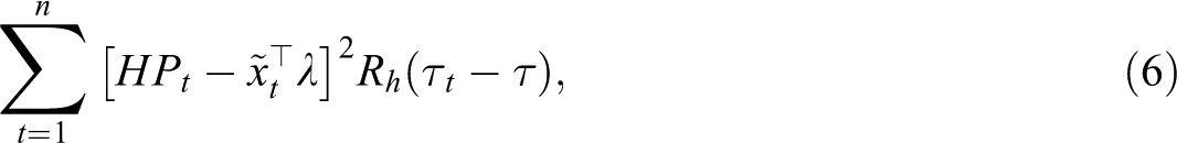
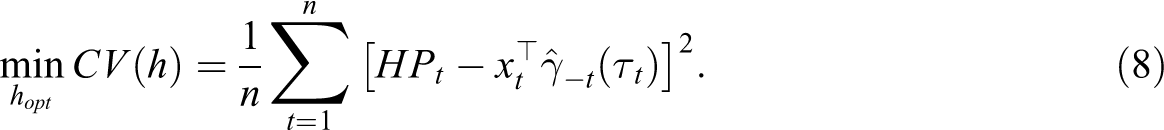
The empirical specification is given by:

where

where n is the sample size and

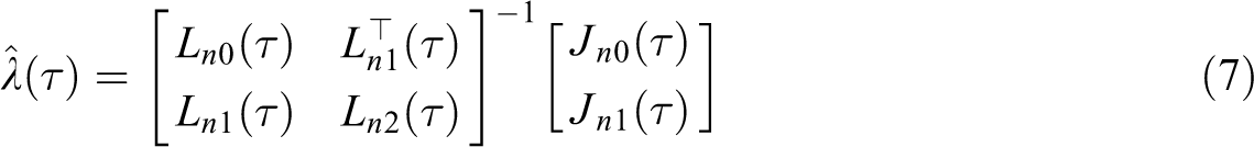
To estimate the coefficient functions, we use the local linear (LL) technique, which has been utilised in the non-parametric literature given its valuable properties such as efficiency, adaptation of boundary effects and bias reduction (Chen et al., 2018b). Under the assumption that each

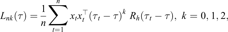
where

where
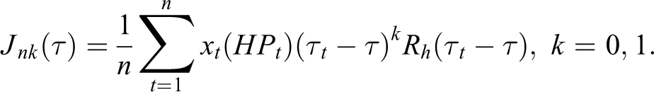
where
with
The LL estimate of
Data
One of the novel features of this article is that it examines the effect of tourism on house prices in Germany over the many decades, which stretches back to the 1870s. The historical time series data is obtained from several sources. Real house prices, real GDP per capita, interest rate, inflation rate, mortgage loans-to-GDP and non-mortgage loans-to-GDP are taken from the Jordà–Schularick–Taylor Macrohistory Database for the period 1870–2016. 4 Data on tourist arrivals from 1870 to 1994 are taken from Rahlf (2016). 5 We update tourist arrival data for the years 1995–2016 from the World Bank’s Development Indicators database. Accordingly, our time series data set consists of annual observations for the period 1870–2016. Table A1 in the Online Appendix details the description and data sources of the variables used.
Standard empirical analyses of time series data utilise parametric techniques that impose linearity assumptions regarding the data generating process and involves satisfying the basic estimation assumptions such as normality, homoscedasticity and no autocorrelation. These assumptions of linearity often lead to using techniques that exhibit low power, despite the fact they may be non-linear. Table 1 presents the descriptive statistics of the time series variables which exhibit volatility in
Descriptive statistics (log-level).
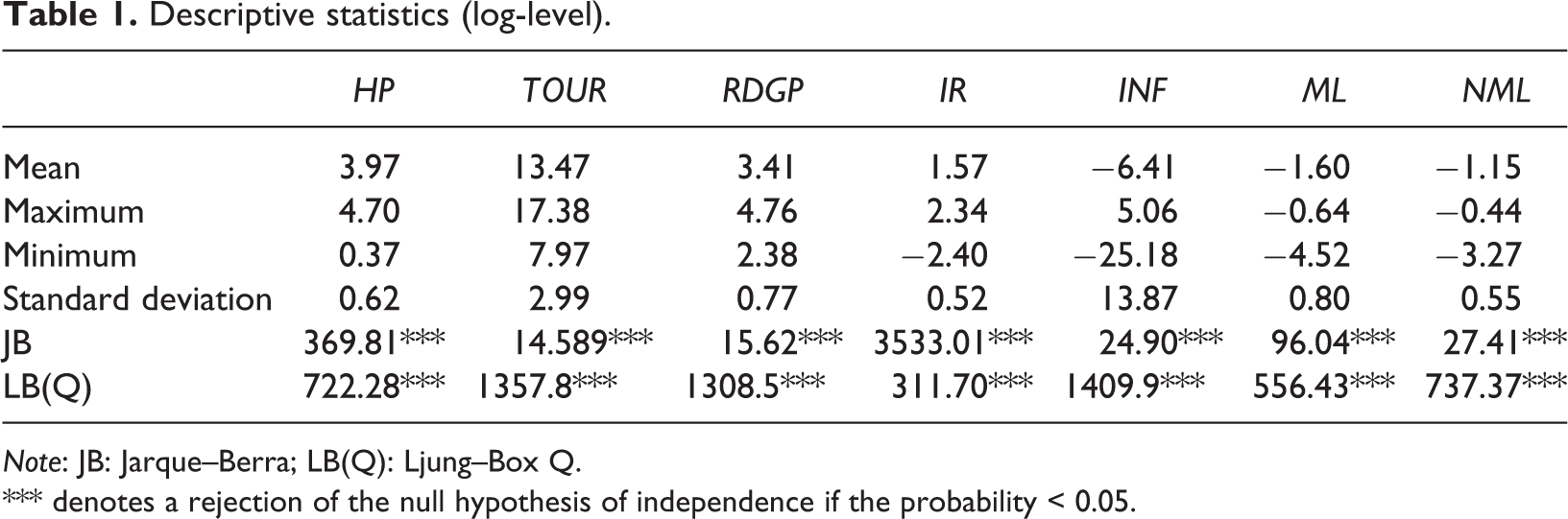
Note: JB: Jarque–Berra; LB(Q): Ljung–Box Q.
*** denotes a rejection of the null hypothesis of independence if the probability < 0.05.
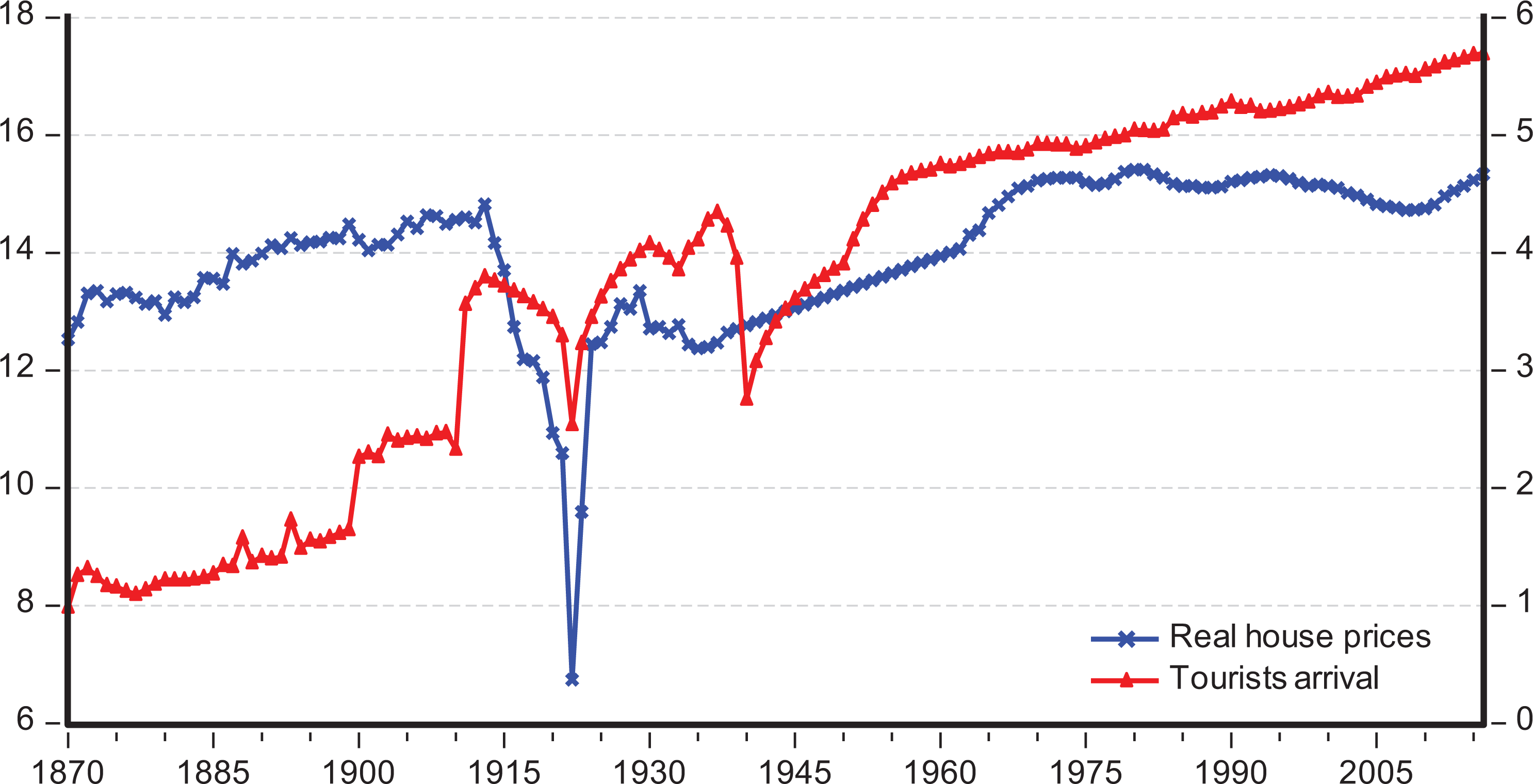
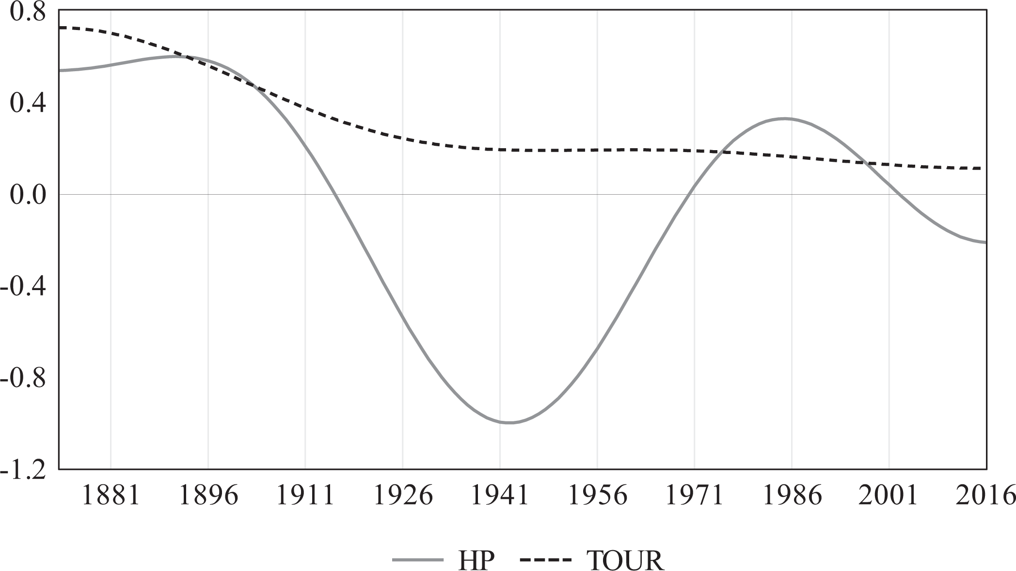
Plot of real house prices (1990 = 100) and tourist arrivals (in logs).
Preliminary analysis
Unit root and time-varying cointegration test
We begin the discussion of the empirical findings with preliminary testing procedures for our time series variables. Conventional analysis of time series data requires testing for stationarity in the variables to determine the order of integration. First, we begin with traditional unit root testing by conducting the augmented dickey–fuller (ADF) unit root test. Second, given the long-run nature of our data, global events such as the world wars and various economic shocks may have caused structural shifts in the variables. Since traditional unit root tests, such as the ADF test, are unable to capture significant structural shifts in the data series, we undertake unit root testing that accommodates for structural breaks. Clemente et al. (1998) develop a test for non-stationarity in the presence of double structural breaks in the series and based on the framework of the additive outlier (AO) and innovative outlier (IO).
Table 2 reports the unit root test results for each variable. Under the ADF test, which includes a constant and a time trend, we find that all variables are non-stationary in levels. Upon first differencing, we find that all variables are stationary (expect for
ADF and Clemente et al. (1998) unit root test.
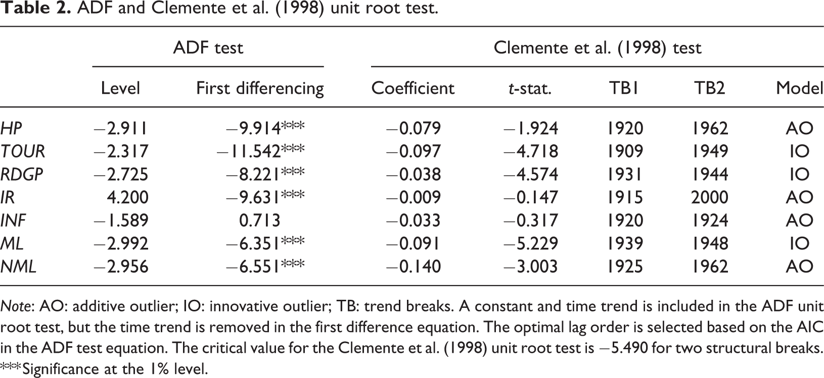
Note: AO: additive outlier; IO: innovative outlier; TB: trend breaks. A constant and time trend is included in the ADF unit root test, but the time trend is removed in the first difference equation. The optimal lag order is selected based on the AIC in the ADF test equation. The critical value for the Clemente et al. (1998) unit root test is −5.490 for two structural breaks.
*** Significance at the 1% level.
Given the non-stationarity of the variables, we procced with examining the cointegrating relationship between
The χ2 distribution with
Bierens and Martins (2010) test for time-varying cointegration.
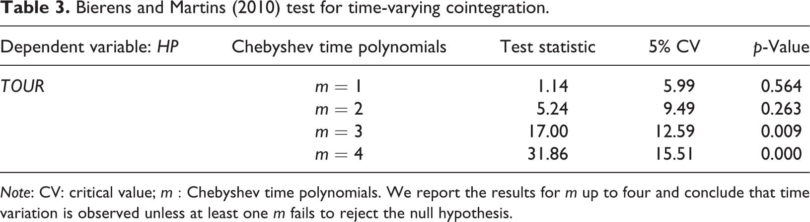
Note: CV: critical value;
Scaled trace statistic of cointegration parameters.
In sum, the findings from the Clemente et al. (1998) unit root test and Bierens and Martins (2010) time-varying cointegration test provide suggestive evidence that the relationship between
Non-linear analysis
Given the findings from the previous section, we test for the existence of a non-linear relationship. Since we observe the presence of time breaks in the variables, we apply the Broock et al. (1996) BDS test. The results from the BDS test are reported in Table 4 and confirm the variables exhibit non-linear dependencies. Based on the test statistics (across the embedded dimensions), the null hypothesis of independent and identically distributed residuals is rejected. Accordingly, this result strongly confirms non-linearity in the time series variables.
BDS non-linearity test.
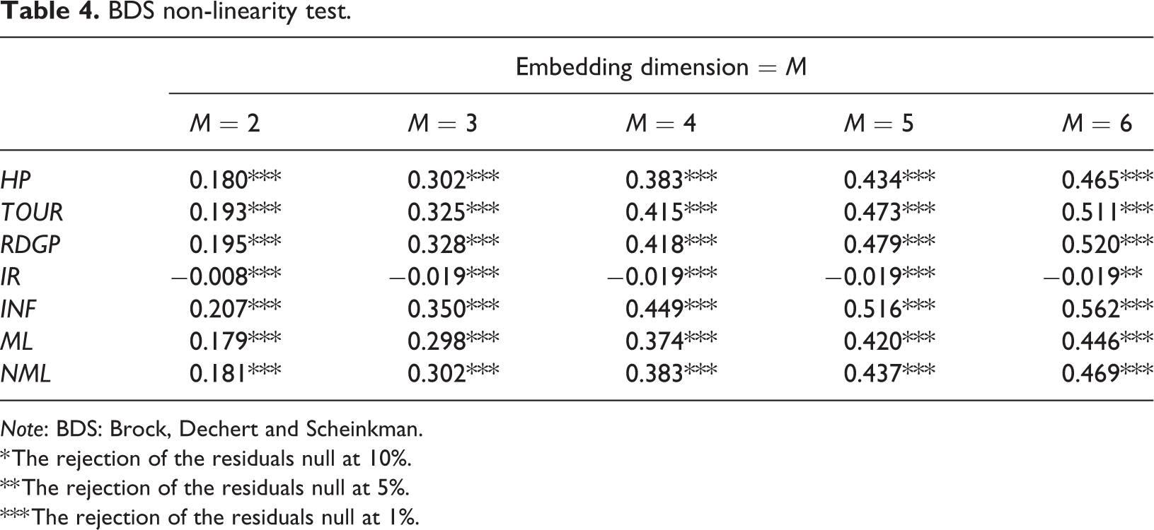
Note: BDS: Brock, Dechert and Scheinkman.
* The rejection of the residuals null at 10%.
** The rejection of the residuals null at 5%.
*** The rejection of the residuals null at 1%.
Next, we apply the Kapetanios et al. (2003) (KSS2003) and Kapetanios and Shin (2008) (KSS2008) non-linear unit root to determine the integration of the variables. The detection of the existence of non-stationarity against non-linear processes is a distinct characteristic of these tests. Given the long span of the data, the use of the non-linear unit root tests is desirable, since the data is characterised by the existence of structural changes and time-varying volatility. The lag length is based on fixed lag and AIC conditions.
Table 5 reports the findings from the KSS2003 and KSS2008 non-linear unit root tests and reveals that the null hypothesis of a unit root in the series is rejected for
Kapetanios et al. (2003) and Kapetanios and Shin (2008) non-linear unit root test.
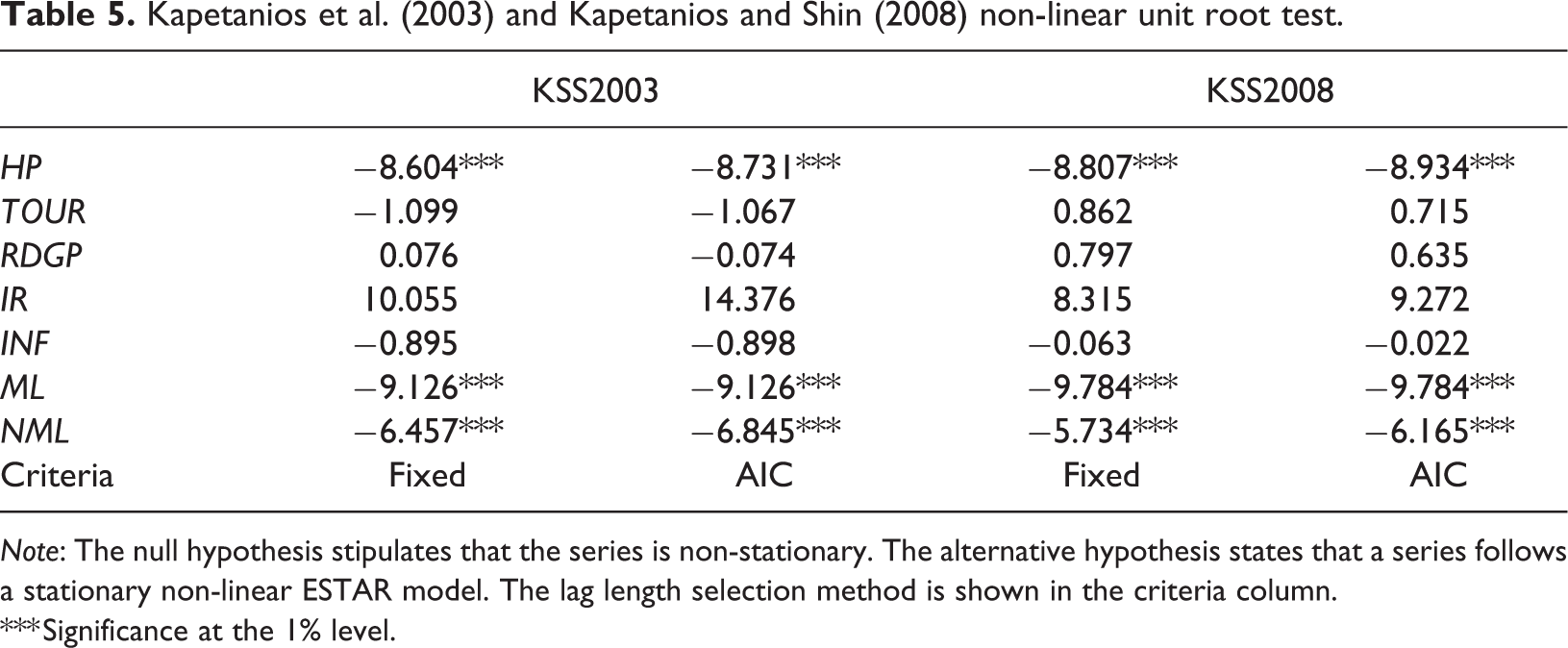
Note: The null hypothesis stipulates that the series is non-stationary. The alternative hypothesis states that a series follows a stationary non-linear ESTAR model. The lag length selection method is shown in the criteria column.
*** Significance at the 1% level.
Based on the mixed evidence on stationarity, we consider whether a cointegrating relationship is present using the non-linear autoregressive distributed lag (NARDL) model. Note that the NARDL model may also be applied regardless of whether the variables are (non-linearly) stationary, non-stationary, or a combination of both. The NARDL technique is also useful as it simultaneously models asymmetries in both the pattern of dynamic adjustment and the long-run relationship. Thus, the negative and positive long-run relationships between the variables of interest are disentangled, and sudden shocks in the series are captured.
The results from the NARDL model are reported in Table 6. Based on the F-test, the results reveal the presence of a long-run asymmetric relationship between
Shin et al. (2014) non-linear ARDL cointegration test.
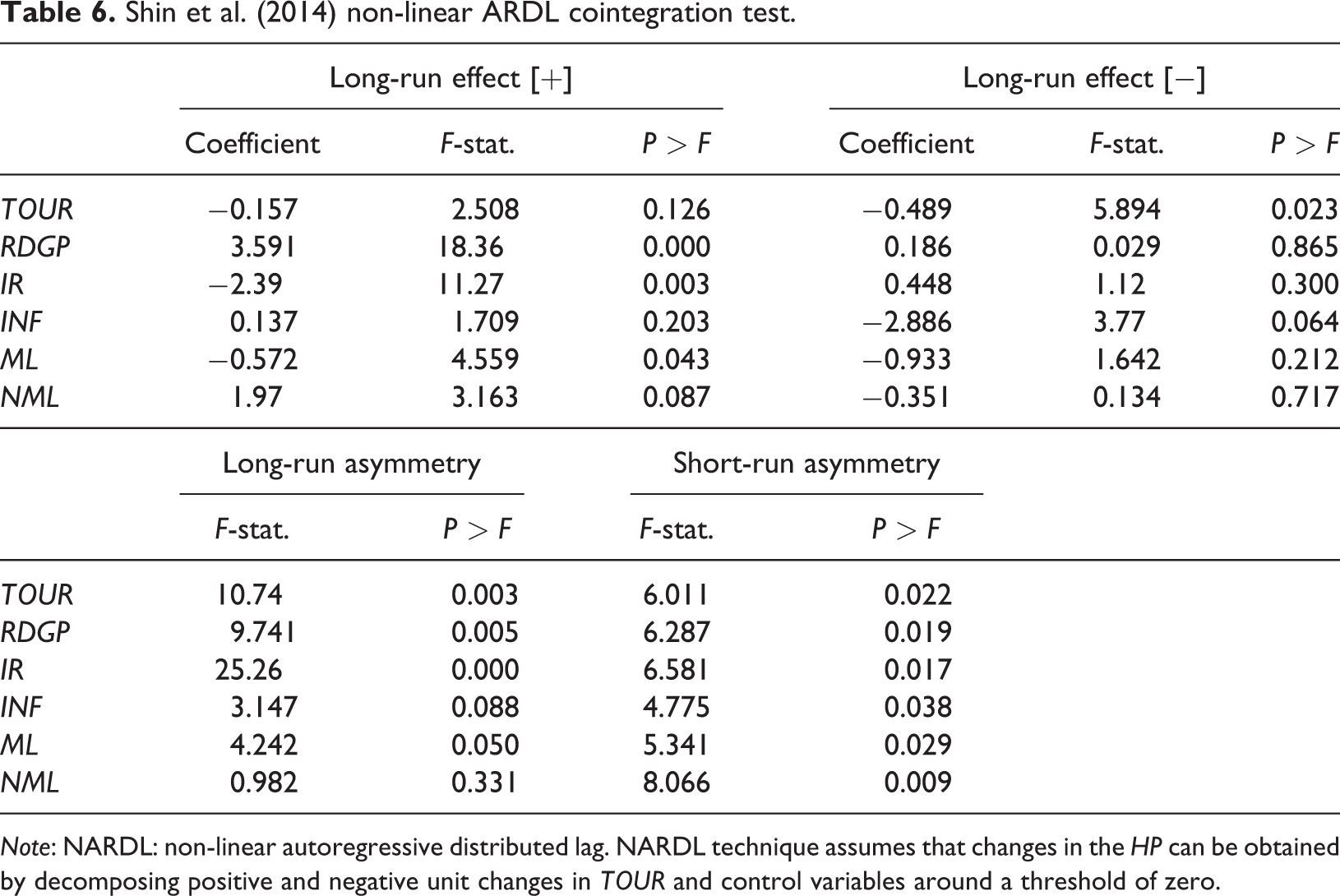
Note: NARDL: non-linear autoregressive distributed lag. NARDL technique assumes that changes in the
Since the results provide evidence for an asymmetric relationship, it becomes necessary to provide more precise estimates of how these changes in
LL TVC results
The findings from the previous section provide evidence of a time-varying relationship and that non-linearities are inherent within the variables. As a result, we now turn to our main analysis by estimating the effects of
The TVC LL estimates are presented in Figure 3 and accompanied by their confidence intervals (90%). In relation to the main variable of interest, we find that
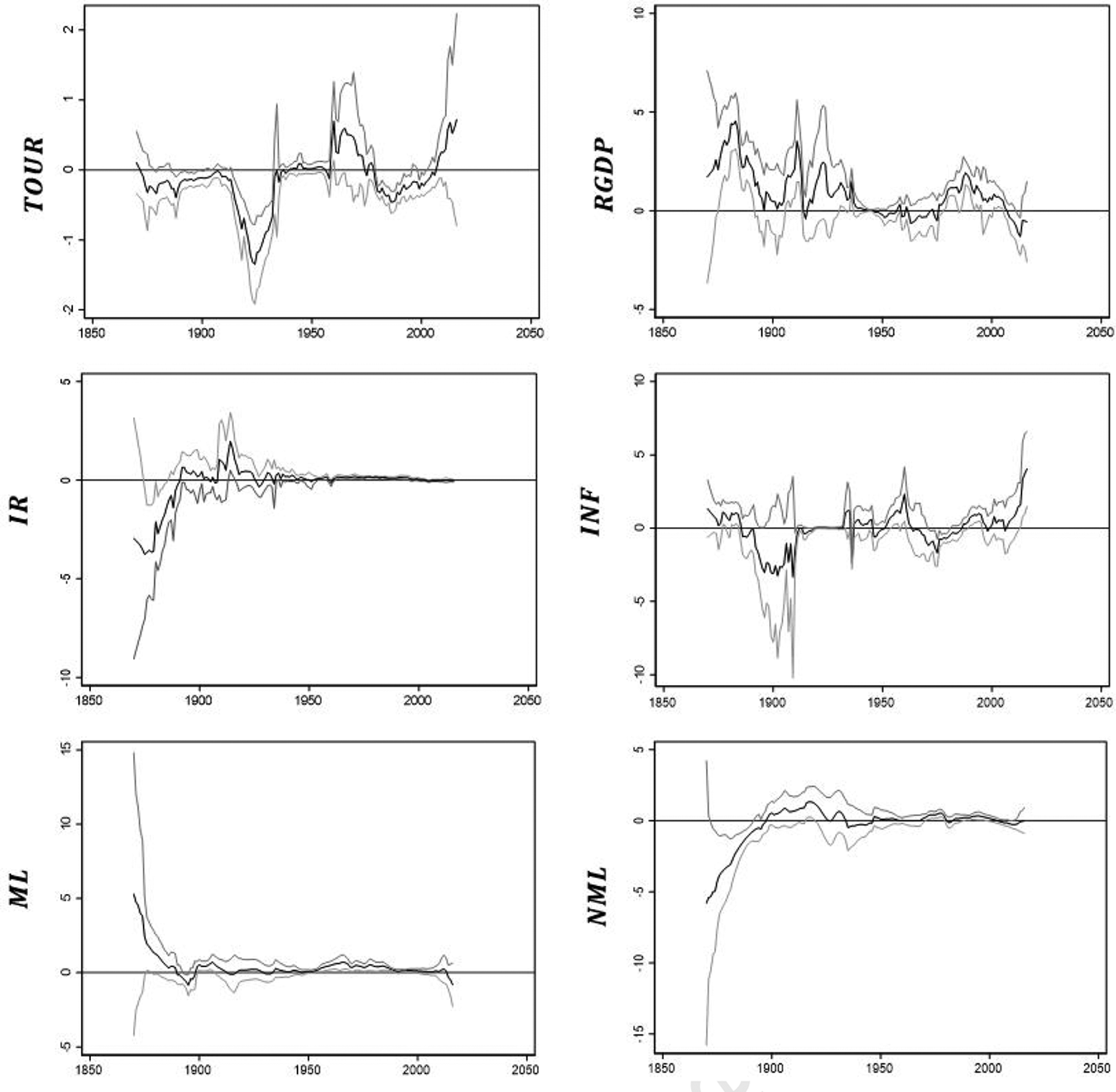
LL TVC estimates (levels). Notes: Dark grey lines denote the 90% confidence interval levels. Black line denotes TVC estimates. TVC: time-varying coefficient; LL: local linear.
From 1935 to 1940, the TVC of
However, the post-1950 period witnessed a surge in the TVC of
Regarding the control variables, for most of the periods under investigation,
Conclusion
This study examined the impact of tourism flows on house prices in Germany since the first globalisation boom of the 1870s. We move beyond traditional parametric techniques and adopt non-parametric methods that track how the tourism–house prices relationship has evolved over time. Our main analysis considers a time-varying non-parametric framework which is more suitable for modelling a dynamic relationship between tourism flows and house prices due to structural breaks caused by global shocks such as the world wars and financial crises, changes in policies, reforms, regulations as well as continued financial development over the many decades.
The initial testing procedures indicate our variables are influenced by abrupt changes due to various economic shocks over the decades and display time-varying characteristics. Based on this evidence, we proceed to determine the non-linear behaviour in the data. We find evidence of an asymmetric relationship between tourism flows and house prices, where negative long-run effects of tourism flows dominate the positive long-run effects for house prices. The main results show a time-varying relationship between tourism and house prices. Tourism has a negative impact on the TVCs on house prices over the early part of the sample period. This negative relationship peaks in the build up to World War II before stabilising during this war period. However, the post-1950 period witnessed a positive relationship between tourism and house prices, albeit for a brief period, after which the effect reverts to a negative relationship up until the mid-1990s. Finally, a second positive relationship if identified between tourism and house prices after 2000 and becomes more pronounced in recent years.
Understanding the dynamic relationship between tourism and house prices is of importance to policymakers. The time-varying relationship between tourism and house prices suggests that other underlying factors mediate the relationship between tourism and house prices and can explain the differential effects over time. Thus, policymakers need to understand the mechanisms through which tourism transmits to house prices to formulate relevant policies. The strong positive effect of tourism on house prices in recent years (i.e. post-2000) could be linked with other externalities, causing an increase in house prices together with tourism growth. While tourism contributes to domestic economic growth, employment and service export (OECD, 2016), many OECD nations, such as Germany, face significant issues of housing affordability coupled with greater tourist flows each year. Policymakers need to find a balance between maintaining growth in the tourism industry and develop regulatory frameworks surrounding real estate properties and accommodation facilities for tourists.
While empirically exploring the mechanisms or channels through which tourism transmits to house prices is beyond the scope of this study, future research can explore these dynamics. There is a general lack of empirical studies on the potential channels through which tourism influences house prices, although these channels can provide meaningful direction for policy. Future research could also focus on other major tourist destination countries in assessing how tourism flows affect house prices or even consider a panel of countries using non-parametric techniques to investigate the time-varying relationship. Several studies have also shown that income inequality may be an important factor that affects tourism–house price nexus (Alam and Paramati, 2016; Paramati and Roca, 2019; Raza and Shah, 2017). Thus, future studies may consider the moderating role of income inequality and tourism on house prices using time-varying non-parametric techniques. Furthermore, while this study considers the effect of tourism on house prices at the country-level, future studies may also consider a within-country (or territorial-level) analysis. An advantage of this type of analysis is that it can reveal the dynamic impact according to the type of region as well as the type of tourism affecting house prices. This, however, does depend on data availability at the regional level.
Supplemental material
Supplemental Material, sj-docx-1-teu-10.1177_13548166211008832 - Has tourism driven house prices in Germany? Time-varying evidence since 1870
Supplemental Material, sj-docx-1-teu-10.1177_13548166211008832 for Has tourism driven house prices in Germany? Time-varying evidence since 1870 by Sefa Awaworyi Churchill, John Inekwe and Kris Ivanovski in Tourism Economics
Footnotes
Declaration of conflicting interests
The author(s) declared no potential conflicts of interest with respect to the research, authorship, and/or publication of this article.
Funding
The author(s) received no financial support for the research, authorship, and/or publication of this article.
Supplemental material
Supplemental material for this article is available online.
Notes
References
Supplementary Material
Please find the following supplemental material available below.
For Open Access articles published under a Creative Commons License, all supplemental material carries the same license as the article it is associated with.
For non-Open Access articles published, all supplemental material carries a non-exclusive license, and permission requests for re-use of supplemental material or any part of supplemental material shall be sent directly to the copyright owner as specified in the copyright notice associated with the article.