Experimental investigation of aerodynamic vibrations of solar wing system

Abstract

The general characteristics of aerodynamic vibrations of a solar wing system were investigated through wind tunnel tests using an aeroelastic model under four oncoming flows. In total, 12 solar panels were suspended by cables and orientated horizontally. Distances between panels were set constant. Tests showed that the fluctuating displacement increases proportionally to the square of the mean wind speed for all wind directions in boundary-layer flows. Larger fluctuating displacements were found for boundary-layer flows with larger power-law indices. Under low-turbulence flow, the fluctuating displacement increased proportionally to the square of the mean wind speed for wind directions between 0° and 30°, but an instability vibration was observed at high mean wind speed for wind directions larger than 40°. And when the wind direction was larger than 60°, a limited vibration was observed at low mean wind speed and the instability vibration was also observed at high mean wind speed. Fluctuating displacements under grid-generated flow showed a similar trend to that of the boundary-layer flows, although the values became much smaller.

Keywords

boundary-layer flow grid-generated flow instability vibration limited vibration low-turbulence flow solar wing system wind tunnel test

Introduction

Fossil fuels have traditionally been used as the dominant energy source for power generation to meet the demands of the growing population for improved lifestyle. The heavy dependence on fossil fuels has severe consequences on the global climate and threatens the balance of the natural environment. Challenges on issues of energy and environmental protection have led to a lot of research and development of clean alternative energy sources to meet energy needs and to reduce fossil fuel consumption and carbon dioxide emissions.

Representative clean energy sources include solar, wind, and biomass, and solar energy is being increasingly used around the world. One widely commercialized solar energy technology is based on photovoltaic solar cells that convert sunlight directly into electricity. Structural design of solar power systems is often governed by wind loads rather than earthquake loads, and wind loads vary significantly depending on the installation method and/or mounting location. Lots of damage to solar panels has been reported because of inadequate estimation of design wind loads, and this has attracted the attention of wind engineers worldwide. As it is difficult to conduct field measurements on solar panels especially on their upper surfaces, and a large number of wind tunnel tests and computational fluid dynamic (CFD) analyses of ground-mounted solar panels have been conducted by numerous researchers (Aly and Bitsuamlak, 2013; Andre et al., 2017; Bitsuamlak et al., 2010; Kopp et al., 2002; Paetzold et al., 2016; Radu and Axinte, 1989; Rohr et al., 2015; Shademan and Hangan, 2009; Somekawa et al., 2013; Strobel and Banks, 2014), some have focused on the characteristics of dynamic wind loading (Andre et al., 2017; Rohr et al., 2015; Strobel and Banks, 2014) and some on the effects of a large geometric scale model (Banks, 2011; Kray and Paul, 2017). And recently in Japan, Manual of Wind Resistant Design for Photovoltaic Systems (Committee of Wind Load Estimation on Photovoltaic System, 2017) was published to help engineers and practitioners to design and maintain solar power systems with higher reliability.

To generate electricity efficiently, solar panels have been mounted on the ground, forming the so-called mega solar power systems. But these systems require huge areas of land, which are very difficult to secure in mountainous and small countries. Thus, alternative systems called solar wing systems or tracking photovoltaic systems have been deployed (Baumgartner et al., 2008, 2009, 2010, 2015). The solar wing system is a new type of installation using cables at both ends, as shown in Figure 1, and the concept and efficiency of this system, including one-axis and two-axis tracking, were introduced by Baumgartner et al. (2008, 2009, 2010, 2015). Theoretically, more than 40% more sunlight can be made available by tracking the solar panels to follow the daily course of the sun relative to the fixed installations. Full-scale measurements have shown that the solar wing system or tracking photovoltaic system offers a gain in yield of up to about 35% relative to fixed mounted photovoltaic installations, depending on the design and the location of the installation. As mentioned, as the solar panels are supported by cables, the solar wing system can be deployed in mountainous areas and in lower seaside areas. Besides, this system has advantages of reduced material costs by reducing the number of mounting platforms and intermediate foundations within the range of the cables. Moreover, it is possible to utilize the ground for other purposes.

Figure 1.

Solar wing system and concept of tracking (Baumgartner et al., 2008).

Table 1 summarizes existing solar wing systems around the world. At present, most are installed near the Germany–Switzerland border. There is also one in South Korea and one in China, which is the one most recently constructed. The ground can be utilized for various purposes, such as waste disposal and storage, because the solar panels are generally installed approximately 5–10 m above ground. Currently, the largest cable length is over 300 m.

Table 1.

Solar wing systems around the world.

Ground usage	Panel height above ground (m)	Cable length (m)	Nominal power (kW)	Since	Location	Tracking system
Parking	4	20	2	2008, 5	Flums, Switzerland	1-axis
Waste disposal site	2	300	654.3	2008, 12	Waldshut, Germany	1-axis
Storage	9	200	90	−	Flums, Switzerland	2-axis
Ski lift	9	320	60.3	2011, 12	Tenna, Switzerland	1-axis
Carport	4	40	420	2012,	Flums, Germany	−
Storage	6	31 (20 layers)	99	2015, 6	Umsung, South Korea	1-axis
Sewage treatment plant	About 5	−	4390	2016, 1	Taizhou, China	1-axis

Although there have been reports on full-scale measurements concerning constructability and productivity of solar wing systems, as the vibrations of cable-supported structures are much more sensitive to wind excitation than earthquake excitation, their aerodynamic characteristics should be carefully investigated in either full scale or model scale. But, to the authors’ knowledge, no such studies have been reported so far. In this article, the aerodynamic characteristics of a solar wing system were investigated through wind tunnel tests using an aeroelastic model under various wind environments, focusing on the variation of fluctuating displacement, power spectrum, and cross-correlations between panels.

Wind tunnel test

Wind tunnel tests were performed in a boundary-layer wind tunnel at Tokyo Polytechnic University in Japan. Its working section is 1.8 m high by 2.2 m wide. Figure 2 outlines the wind tunnel test. In total, 12 solar panels were supported by cables at both ends and the panel size (b × h × D) was 75 mm × 30 mm × 750 mm. They were installed horizontally, not parallel to the cables, and the gaps between panels were set constant. A full-scale structure has six solar modules and supporting members in each panel, but in the experiment they were simply represented by a C-shaped plate made of wood. The length scale was 1/13.3 and the velocity scale was 1/3.7. The mass of one panel was adjusted carefully by considering that of a full-scale one, which includes the mass of six solar modules, supporting members, and cables. Cables with a large Young’s modulus E = 206,000 N/mm² and a diameter of 0.56 mm were used to meet the similarity conditions.

Figure 2.

Outline of wind tunnel test: (a) set-up of solar wing model (low-turbulence flow) and (b) definition of wind direction.

Four laser sensors were installed under a turntable to measure the displacements of solar panels in groups of 2, 5, 8, and 11 (simply, P2, P5, P8, and P11) as shown in Figure 2, and downward displacement was defined as positive. A sag ratio of 2% was used considering that of existing full-scale structures, which is defined as the ratio of sag at the center of the cable to total span length (B). The sampling frequency of the laser sensors was 300 Hz and the measuring time was adjusted such that one 10-min sample was measured. Mean wind speeds U_ref were measured at the tip of the supporting column. To eliminate the effects of the supporting structure on the turntable, tapers were incorporated into its four sides and its inside was also covered by a light board, as shown in Figure 2(a). Wind directions θ from 0° to 90° were considered at 10° intervals, where wind direction 0° is defined as parallel to the model’s short side (Figure 2(b)).

For structures, the shapes of which are affected by gravity, similarity conditions of Froude number F_r and elastic parameter E_s are very important. The Froude number and elastic parameter are defined using equations (1) and (2) and they were satisfied by adjusting the mean wind speeds

F_{r} = \frac{U_{r e f}}{\sqrt{g B}}

(1)

E_{s} = \frac{E A}{B^{2} ρ_{a} U_{r e f}^{2}}

(2)

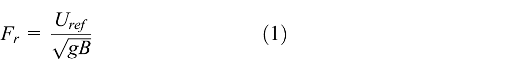
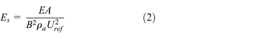
where U_ref is the mean wind speed, g is the gravity acceleration, B is the width, E and A are Young’s modulus and cross-sectional area of the cable, respectively, and ρ_a is the air density.

Four oncoming flows were employed in this study, and the profiles of the oncoming flows are shown in Figure 3. Two boundary-layer flows (BLFs) with power-law indices α = 0.2 and 0.27 were used, and the turbulence intensities at the tip of the supporting column were I_u = 11% and 15%, respectively. Grid-generated flow (GGF) was simulated by placing a grid 0.9 m upstream of the models. The grid size was 0.09 m × 0.09 m and the grid was fixed to the wind tunnel wall and floor during the tests. In the GGF, there was a slight inverse slope in mean wind speed up to about 0.2 m, but the mean wind speed and turbulence intensity were reasonably constant near the panel height. The turbulence intensity at the tip of the supporting column was I_u = 8%. For a low-turbulence flow (LTF), no turbulence-generating apparatuses or spires were used, but because of friction with the wind tunnel floor there were slight slopes in mean wind speed and turbulence intensity up to 0.2 m, the profiles were reasonably constant near panel height. The turbulence intensity at the tip of the supporting column was about I_u = 0.4%. Power spectra of oncoming flows are shown in Figure 3(d). Power spectra for the BLFs show similar tendency and agree well with the Karman spectrum. The power spectra for the GGF and LTF show very different trends from those of BLFs, and for GGF more power is included in the higher frequency range than for LTF.

Figure 3.

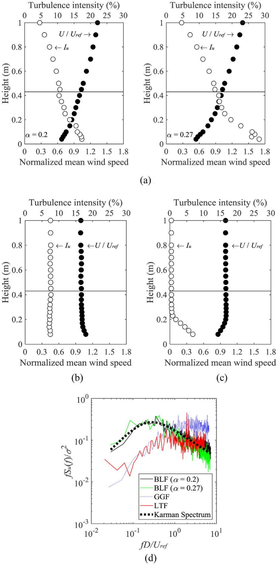
Profiles of oncoming flows: (a) boundary-layer flows (α = 0.2 (left) and 0.27 (right)), (b) grid-generated flow, (c) low-turbulence flow, and (d) power spectra of oncoming flows.

Table 2 summarizes the similarity conditions. A 20-m-long solar wing system of height 5 m above ground was considered. The maximum full-scale mean wind speeds up to 26 m/s for BLF and 37 m/s for GGF and LTF at 5 m were considered, but the maximum wind speeds under GGF and LTF were limited by severe vibrations depending on the wind direction.

Table 2.

Similarity conditions.

	Full-scale	Model-scale	Scale
Length B (m)	20	1.5	1/13.3
Width D (m)	9.95	0.75
Height H (m)	5	0.38
Panel width b (m)	0.99	0.07
Panel height h (m)	0.34	0.03
Total weight (N)	64,331	27.3	(1/13.3)³
Weight of one panel (N)	5361	2.26	(1/13.3)³
Mean wind speed (m/s)	~26 (BLF) or 37 (GGF and LTF)	~7 (BLF) or 10 (GGF and LTF)	1/3.7

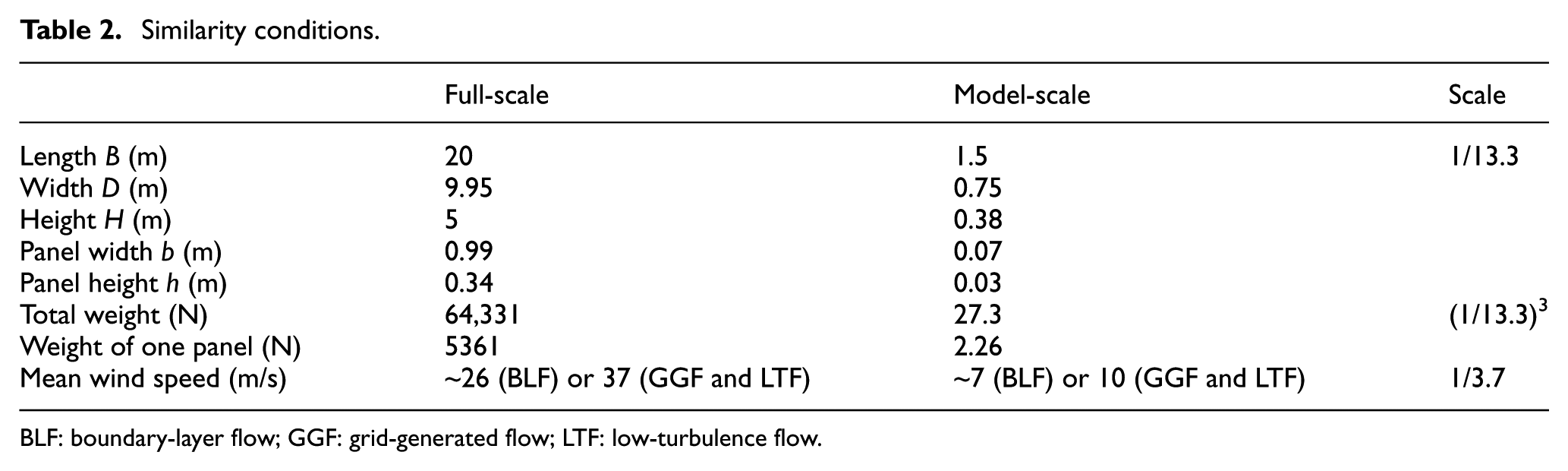
BLF: boundary-layer flow; GGF: grid-generated flow; LTF: low-turbulence flow.

System properties were obtained from free vibration tests with no wind condition, and the first three natural frequencies and damping ratios in the vertical direction were about 3.9, 5.7, and 8.6 Hz, and 0.28%, 0.14%, and 0.1%, respectively.

Results and discussion

Figure 4 shows the variation of fluctuating displacements for wind direction 0° for the BLF with α = 0.2. The abscissa indicates the mean wind speed measured at the tip of the supporting column and the ordinate indicates the normalized fluctuating displacements by column height (σ/H). The fluctuating displacements are defined as the standard deviation of the time series. Symbols in the figure represent panel positions (Figure 4(a)) and wind directions (Figure 4(b)). The fluctuating displacements increase moderately with mean wind speed regardless of panel positions, and the inner panels (P5 and P8) show larger values than the outer panels (P2 and P11). The increase is almost proportional to the square of mean wind speed. As the wind direction increases, the fluctuating displacement increases up to wind direction 30°, and after showing a maximum value at 30°, the fluctuating displacement decreases and becomes similar to that for wind direction 0°.

Figure 4.

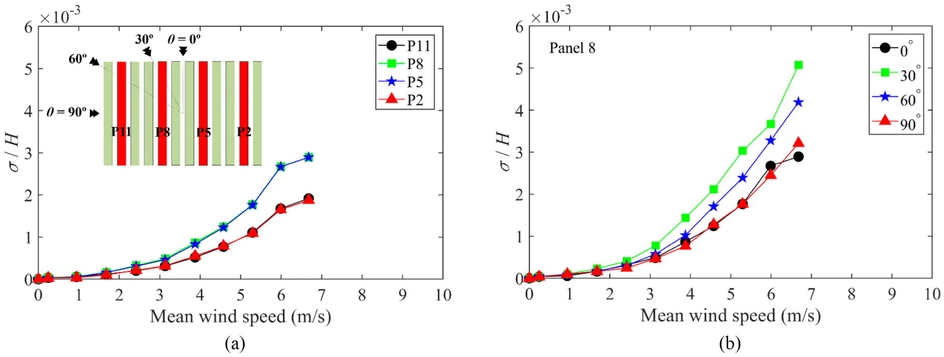
Variation of fluctuating displacement for BLF with α = 0.2: (a) wind direction of 0° and (b) panel 8.

Figure 5 shows the variation of fluctuating displacements for the BLF with α = 0.27. A similar trend was found to the BLF with α = 0.2, showing a moderate increase with mean wind speed and also maximum values at wind direction 30°. From Figures 4 and 5, it was found that the fluctuating displacement under the BLFs corresponds to a buffeting vibration, being proportional to the square of mean wind speed.

Figure 5.

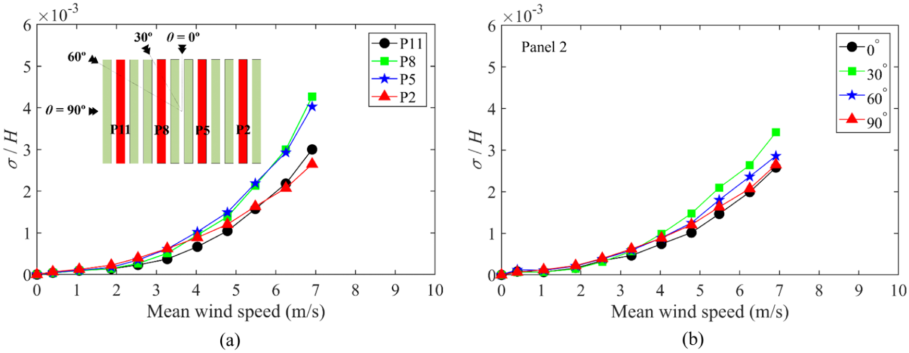
Variation of fluctuating displacement for BLF with α = 0.27: (a) wind direction of 90° and (b) panel 2.

Figure 6 shows the fluctuating displacement under GGF. As shown, it increases moderately with mean wind speed for all wind directions such as those under BLFs, but few differences were found in panels and wind directions. The fluctuating displacement also corresponds to the buffeting vibration, even though the values and slope are smaller than those under BLFs.

Figure 6.

Variation of fluctuating displacement for GGF: (a) wind direction of 90° and (b) panel 11.

Fluctuating displacement in LTF for various wind directions is shown in Figure 7. When the wind direction is 0° (Figure 7(a)), fluctuating displacement increases moderately with mean wind speed and wind direction. A moderate increase is found up to wind direction 30°. As the wind direction increases (Figure 7(b)), a sudden increase is observed near the mean wind speed of 9 m/s (about 33 m/s in full scale), and at the next step one of the cables was cut on account of severe vibrations. These kinds of instability vibrations were observed at relatively high mean wind speeds when the wind direction was larger than 40°. For the following tests for LTF, when a sudden increase occurred in any of the solar panels, the test was stopped and moved to the next wind direction. As the wind direction increases further (Figure 7(c)), a sudden increase is observed near the mean wind speed of 1.5 m/s (about 5 m/s in full scale) and near 6 m/s (about 22 m/s in full scale). For the sudden increase near the mean wind speed of 1.5 m/s, the fluctuating displacements greatly decrease at the next step, implying that the increase is a kind of limited vibration such as vortex-shedding vibration. Limited vibration is clearly observed when the wind direction is larger than 50° near the mean wind speed of 1.5 m/s, and there is little effect of fairing on reducing the limited vibration near the mean wind speed of 1.5 m/s (Tamura et al., 2015). Comparison of fluctuating displacement with wind direction is shown in Figure 7(d). For wind directions from 0° to 30°, buffeting-like vibrations were observed and instability vibrations occurred at high mean wind speed for wind directions larger than 40°. The mean wind speeds at which the instability vibrations occurred decrease with increasing wind direction. Limited vibrations were clearly seen for wind directions larger than 50° near the mean wind speed of 1.5 m/s regardless of panel positions. In this study, limited vibrations were only observed under LTF near the mean wind speeds of 1.5 m/s.

Figure 7.

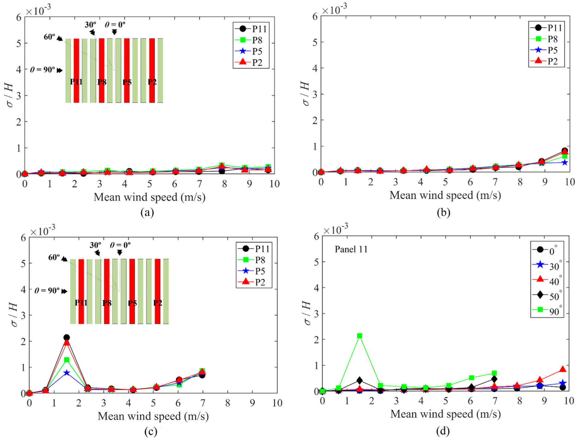
Variation of fluctuating displacement for LTF: (a) wind direction of 0°, (b) wind direction of 40°, (c) wind direction of 90°, and (d) panel 11.

Figure 8 shows the fluctuating displacements of P8 and P11 for wind directions 0° and 90°. For wind direction 0°, the fluctuating displacement increases with mean wind speed and those under BLF are much larger than those under GGF and LTF, showing the smallest values for LTF. For the BLFs, the larger the power-law index, the larger the fluctuating displacement. A similar trend was found for wind direction 90°, but a clear limited vibration under LTF was found and the fluctuating displacements for GGF and LTF became similar.

Figure 8.

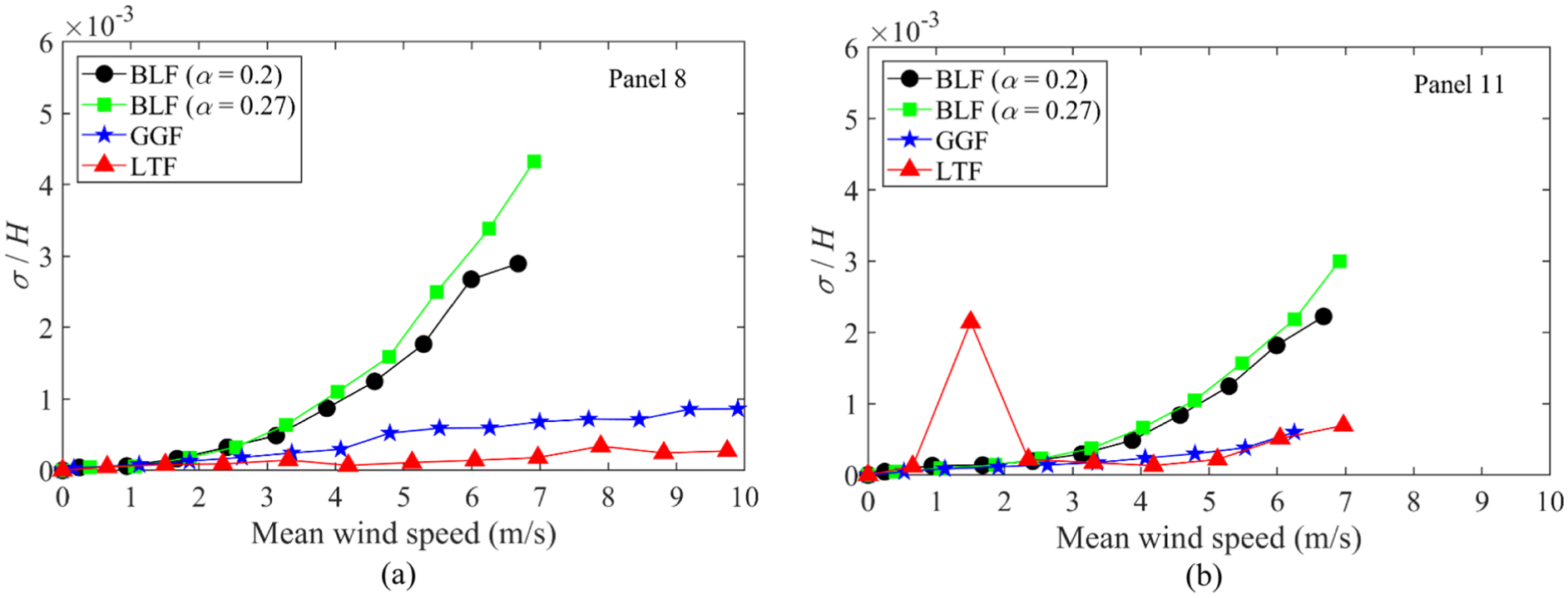
Comparison of fluctuating displacements under different oncoming flows: (a) wind direction of 0° and (b) wind direction of 90°.

As shown in Figures 7 and 8, limited vibrations occurred near mean wind speed 1.5 m/s under LTF and an additional test was conducted to examine their characteristics. The procedure was as follows. As shown in Figure 9, first all intervals between solar panels were covered by very light sheets and the occurrence of limited vibration was examined at mean wind speed 1.5 m/s. When all intervals between solar panels were covered, no limited vibration occurred, implying that the intervals between solar panels are related to the occurrence of limited vibration. Then, only a light sheet (11) in Figure 9 was removed, leaving the rest of the light sheets covered, and the occurrence of limited vibration was re-examined at mean wind speed 1.5 m/s. When a panel interval (11) was open, no limited vibration occurred. Next, a light sheet (10) was removed (intervals (11) and (10) were open in this state), leaving the rest of the light sheets covered, and the occurrence of limited vibration was examined again. In this way, the light sheets were removed one by one from the upstream side and the occurrences of limited vibration were examined. The results are summarized in Table 3. As shown, when one of the intervals of (1) and (2) or both were open regardless of the other intervals, limited vibrations occurred, meaning that the phenomena that occurred in intervals (1) and/or (2) are related to the limited vibration.

Figure 9.

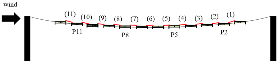
Covering intervals between solar panels (wind blows from left to right).

Table 3.

Position of light sheets and occurrence of limited vibration.

Position of light sheets	Opening of panel intervals	Occurrence of limited vibration
(1)~(11)	All closed	Not occurred
(1)~(10)	(11) open	Not occurred
(1)~(9)	(11)~(10) open	Not occurred
(1)~(8)	(11)~(9) open	Not occurred
(1)~(7)	(11)~(8) open	Not occurred
(1)~(6)	(11)~(7) open	Not occurred
(1)~(5)	(11)~(6) open	Not occurred
(1)~(4)	(11)~(5) open	Not occurred
(1)~(3)	(11)~(4) open	Not occurred
(1)~(2)	(11)~(3) open	Not occurred
(1)	(11)~(2) open	Occurred
(2)	All open except (2)	Occurred
No light sheets	All open	Occurred

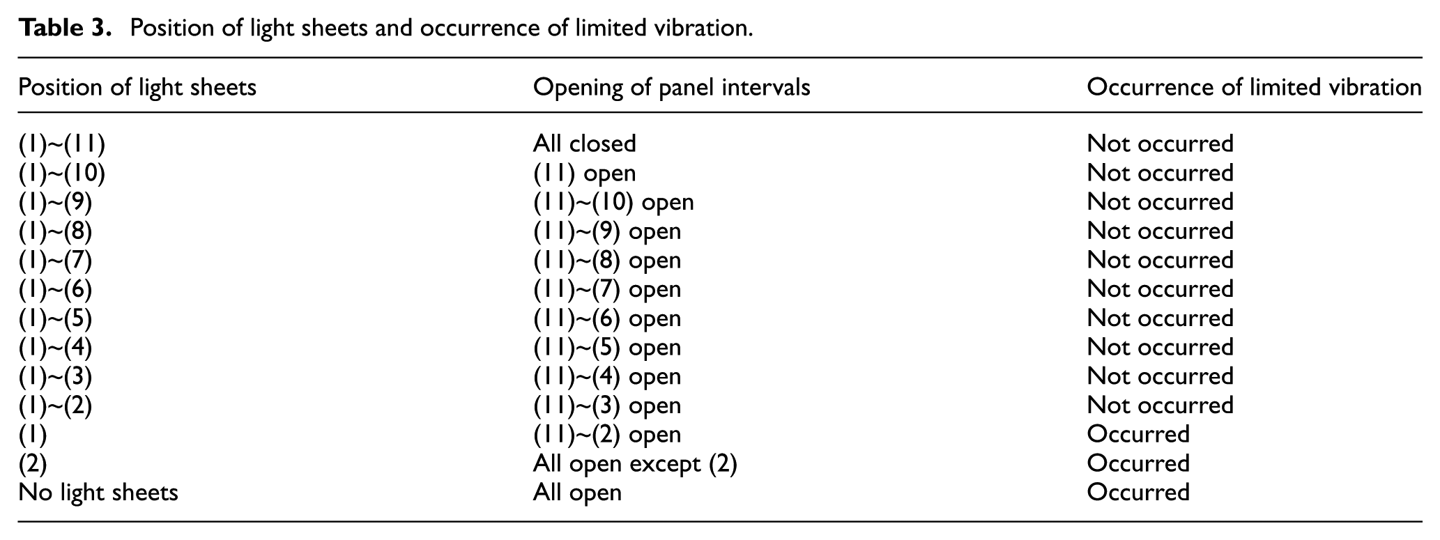
Figure 10 shows the power spectra of fluctuating displacement for various wind speeds under different oncoming flows (P2). Note that the axes were not normalized and the areas under the power spectra correspond to the variance of the time series. There are some peaks near the system’s natural frequencies, and the power becomes larger for higher mean wind speed for BLF regardless of wind direction (Figure 10(a) and (b)). A similar trend was found for LTF in Figure 10(c) and (d), but when the limited vibration occurs the peak of the 3rd mode becomes much larger than those of other power spectra, meaning that the limited vibration is a resonant phenomenon in the 3rd mode. In Figure 10(d), the black line indicates the power spectrum at the mean wind speed just before the limited vibration, the red line indicates that at the limited vibration, and the green line indicates that right after the limited vibration. Normalized frequency for the limited vibration by mean wind speed U_ref and panel height h, which can be defined as the Strouhal number (fh/U_ref), is 0.177. As the resonant vibration is always related to the vortex shedding, it can be imagined that the panel intervals of (1) and (2) are important in the vortex formation and shedding. The power spectra of GGF show similar shapes to those of BLFs, and by considering turbulence in oncoming flows it can be found that the vortex formation between panels becomes weak or disturbed.

Figure 10.

Characteristics of power spectra under different oncoming flows (P2): (a) under BLF of α = 0.2 (θ = 0°) for various mean wind speeds; (b) under BLF of α = 0.2 (θ = 90°) for various mean wind speeds; (c) under LTF (θ = 90°) for various mean wind speeds; and (d) under LTF (θ = 90°) near the limited vibration.

Figure 11 shows the cross-correlation coefficient between P11 and P2 (ρ_P11-P2), which are located at both outer sides, for various wind speeds under different oncoming flows. The abscissa is a normalized time lag normalized by mean wind speed U_ref and width D of the system (Figure 1). For wind direction 0° under BLF (Figure 11(a)), the correlations show a kind of periodic trend and the period becomes large and correlations seem to become small with increasing mean wind speed. When the wind direction becomes 90° (Figure 11(b)), the periodic trends collapse and correlations become small. On the other hand, the correlations in LTF are very high, but decrease with increasing mean wind speed (Figure 11(c)) at wind direction 0°. When the wind direction becomes 90° (Figure 11(d)), periodic characteristics can be observed and the correlation amplitude is very large when the limited vibration occurs, implying that the vibrations of P11 and P2 are governed by a periodic vortex excitation. For high mean wind speeds, the periodic characteristics remain, but the periods and correlations become different. As the periodic trends under BLF in Figure 11(a) are not as clear as those under LTF in Figure 11(d), the excitation characteristics are considered to be different from each other.

Figure 11.

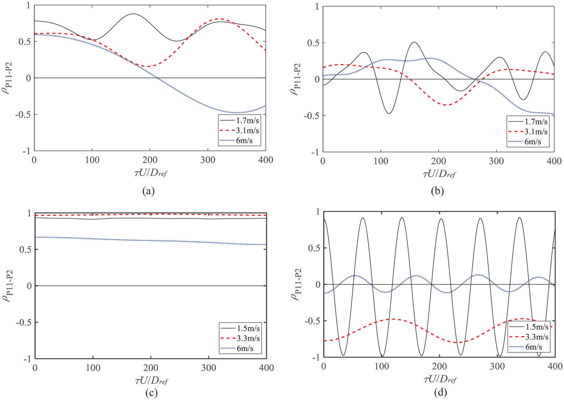
Comparison of cross-correlation coefficients between P11 and P2 under different oncoming flows: (a) under BLF of α = 0.2 (θ = 0°) for various mean wind speeds; (b) under BLF of α = 0.2 (θ = 90°) for various mean wind speeds; (c) under LTF (θ = 0°) for various mean wind speeds; and (d) under LTF (θ = 90°) for various mean wind speeds.

Concluding remarks

The general characteristics of aerodynamic vibrations of a solar wing system were investigated through wind tunnel tests using an aeroelastic model under four different oncoming flows. Fluctuating displacements for BLF and GLF show very similar trends for all wind directions. However, very different and characteristic vibrations were found for LTF.

For BLF and GLF, fluctuating displacements increase linearly with the square of mean wind speed (buffeting vibration), and a similar trend was also found for LTF for wind directions between 0° and 30°.

For LTF, an instability vibration was found at high mean wind speed for wind directions larger than 40°, meaning that there is a possibility of system collapse on account of instability vibration for a certain wind direction. In this study, the mean wind speed at which instability vibration occurs was about 37 m/s for wind direction 40° and the mean wind speed became small with increasing wind direction. When the wind direction was larger than 50°, limited vibration was found at low mean wind speed as well as instability vibration at high mean wind speed. The full-scale mean wind speed for limited vibration corresponds to about 5 m/s, and as this mean wind speed is expected to occur daily, fatigue damage may accumulate, again resulting in a possibility of system collapse under daily wind. The limited vibration is thought to be a higher mode resonant vibration (especially, 3rd mode), which can be suppressed by adding damping, and intervals between panels located on the downstream side are found to be important to the occurrence of limited vibration. By considering turbulence in oncoming flows, the vortex formation between panels becomes weak or disturbed.

The importance of simulation of realistic oncoming flow can well be understood from this study again, and for areas with small slopes in mean wind speed and turbulence intensity and with very low turbulence intensity similar to LTF, the construction of solar wing systems should be carefully examined in various aspects.

Footnotes

Author’s Note

Q Yang is now affiliated to School of Civil Engineering, Beijing Jiaotong University, Beijing, P.R. China and School of Civil Engineering, Chongqing University, Chongqing, P.R. China.

Declaration of Conflicting Interests

The author(s) declared no potential conflicts of interest with respect to the research, authorship, and/or publication of this article.

Funding

The author(s) disclosed receipt of the following financial support for the research, authorship, and/or publication of this article: This study was funded by the Ministry of Education, Culture, Sports, Science and Technology, Japan, through the Global Center of Excellence Program, 2008-2012 (H13), and 111 Project and 1000 Foreign Talent Program, China (B13002). The authors gratefully acknowledge their support.

References

Aly

Bitsuamlak

(2013) Aerodynamics of ground-mounted solar panels: test model scale effects. Journal of Wind Engineering and Industrial Aerodynamics 123: 250–260.

Andre

Péntek

Bletzinger

et al . (2017) Aeroelastic simulation of the wind-excited torsional vibration of a parabolic trough solar collector. Journal of Wind Engineering and Industrial Aerodynamics 165: 67–78.

Banks

(2011) Measuring peak wind loads on solar power. In: Proceedings of the 13th international conference on wind engineering, Amsterdam, 10–15 July.

Baumgartner

Büchel

Bartholet

(2008) Solar wings: a new lightweight photovoltaic tracking system. In: Proceedings of the 23th European photovoltaic solar energy conference, Valencia, 1–5 September, 4DO.9.5.

Baumgartner

Büchel

Bartholet

(2009) Experiences with cable-based solar wings tracking system and progress towards two-axis large scale solar systems. In: Proceedings of the 24th European photovoltaic solar energy conference, Hamburg, 21–24 September, 4CO.8.6.

Baumgartner

Büchel

Bartholet

(2010) Cable-based solar wings tracking system: two-axis system and progress of one-axis system. In: Proceedings of the 25th European photovoltaic solar energy conference, Valencia, 6–9 September, 4BV.1.34.

Baumgartner

Büchel

Bartholet

(2015) Solar ski lift PV carport and other solar wings cable based solutions. In: Proceedings of the 27th European photovoltaic solar energy conference, Frankfurt, 25 September, 4BV.1.60.

Bitsuamlak

Dagnew

Erwin

(2010) Evaluation of wind loads on solar panel modules using CFD. In: 5th international symposium on computational wind engineering, Chapel Hill, NC, 23–27 May.

Committee of Wind Load Estimation on Photovoltaic System (2017) Manual of Wind Resistant Design for Photovoltaic System. Tokyo: Japan Association for Wind Engineering and Joint Usage/Research Center, Tokyo Polytechnic University (in Japanese).

10.

Kopp

Surry

Chen

(2002) Wind loads on solar array. Wind and Structures 5(5): 393–406.

11.

Kray

Paul

(2017) Peak negative pressure coefficients on low-tilted solar arrays mounted on flat roofs: the effects of building size and model scale. In: Proceedings of the 7th European-African conference on wind engineering, Liège, 3–6 July.

12.

Paetzold

Cochard

Fletcher

et al . (2016) Wind effects in solar fields with various collector designs. AIP Conference Proceedings 1734(1): 020018-1–020018-8.

13.

Radu

Axinte

(1989) Wind forces on structures supporting solar collectors. Journal of Wind Engineering and Industrial Aerodynamics 32: 93–100.

14.

Rohr

Bourke

Banks

(2015) Torsional instability of single-axis solar tracking systems. In: Proceedings of the 14th international conference on wind engineering, Porto Alegre, 21–26 June.

15.

Shademan

Hangan

(2009) Wind loading on solar panels at different inclination angles. In: 11th American Conference on Wind Engineering, San Juan, 22–26 June.

16.

Somekawa

Taniguchi

Taniike

(2013) Wind loads acting on PV panels and support structures with various layouts. In: 8th Asia-Pacific conference on wind engineering, Chennai, India, 10–14 December.

17.

Strobel

Banks

(2014) Effects of vortex shedding in arrays of long inclined flat plates and ramifications for ground-mounted photovoltaic arrays. Journal of Wind Engineering and Industrial Aerodynamics 133: 146–149.

18.

Tamura

Kim

Yoshida

et al . (2015) Wind-induced vibration experiment on solar wing. In: 6th international conference on experimental vibration analysis for civil engineering structures, Zurich, 19–21 October.