Suspension bridge response assessment under temperature-vehicle combined loading: An analytical algorithm

Abstract

Suspension bridges’ excellent spanning capacity is compromised by their insufficient stiffness, making their live load response quite challenging. This study introduces an analytical method for solving the response of the suspension bridge under the temperature-vehicle combined loading. The deformation of the main cable is estimated based on the elastic catenary theory. The variation of internal forces expresses the pylon’s and the beam’s deformation. Displacements of key nodes are estimated and set as constraints. Given the high non-linearity and complexity of suspension bridges, the residual sum of squares of all constraints is the objective function in an optimization algorithm. The analytical solutions to the system of equations are found by employing the generalized reduced gradient method (GRG), yielding deformations and internal forces of the suspension bridge. The proposed method demonstrates high computational efficiency and accuracy, achieving a computation time of less than 1 min for a 1700 m suspension bridge and a maximum vertical displacement error of only 0.59%. Further analysis reveals that the coupling effect between temperature and vehicle loads has a limited impact on vertical displacement calculations but causes a non-negligible influence on beam-end rotations. These findings highlight the necessity of considering temperature-vehicle interaction in suspension bridge assessment to ensure more precise and reliable predictions.

Keywords

suspension bridge analytical method thermal behavior live load elastic catenary cable

Introduction

Given the high non-linearity (Ribeiro et al., 2024) and small stiffness of suspension bridges, live load response remains a key consideration at both the design and service periods. Railway suspension bridges have emerged in recent years, which raises a higher demand for refined theories of live load design. Compared with the highway suspension bridge, the railway suspension bridge has two distinctive features: (1) The railway suspension bridge is subject to greater moving loads. According to the Chinese bridge standards, the lane loads on highways and railways should consider a uniformly distributed load 10.5 kN/m and 36.8 kN/m to 41.7 kN/m, respectively. (2) Compared with automobiles, high-speed trains have a higher requirement for track smoothness. The reasons are two-fold. First, high-speed trains are expected to meet higher safety and comfort requirements; second, track irregularity is the main source to induce the vibration of the vehicle-track system, which causes damage to the train parts and track structure and dramatically increases safety risks and maintenance costs (Grigorjeva et al., 2006; Shi et al., 2022). Therefore, precise calculation of live load response is indispensable for the design of the suspension bridge.

The conventional theories for estimating the live load response have undergone three stages of evolution. That is, from the elastic theory (Gasparini and Buonopane, 2019; Rankine and Millar, 1921; Steinman, 1929) to the deflection theory (Cobo del Arco and Aparicio, 2001; Choi et al., 2013; Choi et al., 2014; Zhuang et al., 2021) and finally to the finite displacement theory (Fleming, 1979; Lonetti and Pascuzzo, 2016; Saafan, 1966). However, these theories have their respective limitations. The elastic theory assumes that the main cable shape does not change under the live load, thus neglecting the contribution made by the dead load to the stiffness of the suspension bridge. For this reason, the elastic theory usually results in an overly conservative design. The deflection theory represents a substantial improvement and remains a cornerstone theory for estimating the live load response of the suspension bridge. One defect with the deflection theory is that the hangers are simplified into uniform membranes, and the main cable shape is assumed to be parabolic. In addition, the deflection theory neglects hanger deformations under the live load. All of the above simplifications will have a non-negligible impact on the accuracy of the calculation results when the bridge deformations are significant (Li and Luo, 2023). The finite displacement theory introduces the concepts of elements and matrix into live load response estimation of the suspension bridge, which helps improve the accuracy. The finite displacement theory has become a mainstay in suspension bridge design. However, it heavily depends on matrix operations and does not give clear physical parameter definitions. Besides, the complex iterative procedures involved in the finite element method are likely to result in low efficiency in the case of a large-scale suspension bridge (Kim and Thai, 2011; Sgambi et al., 2012). Recently, refined analytical methods have been proposed to solve the live load response of suspension bridges (Jung et al., 2015; Li and Luo, 2023; Shin et al., 2015; Zhang et al., 2021).

Unfortunately, most analytical methods (Zhang et al., 2025) used for calculating the live load response (Ma et al., 2025) of suspension bridges focus on vehicle loads, disregading effects of other factors, e.g., temperature-induced stresses (Jing et al., 2024) that arise at the operation stage. In fact, the suspension bridge is always subjected to the temperature-vehicle combined loading (Marchenko et al., 2024). Thermal load has a non-negligible impact on the live load response of the suspension bridge, primarily due to the following reasons: (1) Thermal load will significantly change the shape of the main cable, which in turn affects the mechanical properties of the suspension bridge decisively, such as structural stiffness and natural vibration frequency (Sun et al., 2009). Therefore, thermal load inevitably affects the response of the suspension bridge under the vehicle load. (2) The pylon deformation caused by thermal load will change the coordinates of the main cable’s intersection point (IP), which further affects the shape and mechanical properties of the main cable. Notably, the pylons undergo a significant P-delta effect under the temperature-vehicle combined loading, amplifying the IP’s displacement in the main cable. Calculating the live load response of the suspension bridge without considering the thermal load will induce significant errors.

As suspension bridges are flexible systems, their geometric shape and internal forces are highly sensitive to temperature. The thermal effects on suspension bridges have long been a concern in the engineering community. With increasing bridge spans, temperature-induced stresses and deformations become non-negligible compared to dead load and live load effects. Many scholars have conducted research in this field, and current approaches for studying thermal effects can generally be divided into three categories.

The first method involves numerical simulation using finite element analysis to evaluate environmental temperature impacts on structures. Fan et al. (2009) analyzed the effect of a non-uniform solar temperature field on the cable-net structure of the reflector for the Five-hundred-meter Aperture Spherical Radio Telescope (FAST) using the thermal analysis module of ANSYS. (Zhu et al., 2023) simulated the non-uniform temperature field and its effects on truss suspension railway bridges under solar radiation. Ray et al. (2025) studied the characteristics of fiber-reinforced-plastic bridge decks under combined thermal and vehicle loads through finite element modeling.

The second approach utilizes Structural Health Monitoring (SHM) systems to assess non-uniform temperature distributions in bridges by fitting functions to long-term monitoring data. Xu et al. (2010) monitored temperature effect and load response of The Tsing Ma Bridge using wind and structural health monitoring system. Yang et al. (2024) conducted a series of studies on temperature-induced bridge responses based on SHM system data, identifying a strong linear relationship between structural temperature and deformation. They also proposed a method for expanding bridge temperature datasets using meteorological parameters. Zhu et al. (2024) analyzed temperature field characteristics and temperature-induced effects on steel girders and track alignment through SHM models, field tests, and numerical simulations. However, regression analysis methods relying on bridge monitoring data may incur higher economic costs, as the scale and quality of datasets directly affect the effectiveness and accuracy of thermal behavior analysis.

The third method employs analytical solutions to determine bridge thermal effects. Zhang et al. (2019) proposed an analytical method for modeling temperature sensitivity in suspension bridge cable configurations. Wang et al. (2023) developed an analytical solution for thermal effects on suspension bridges using a surrogate model with longitudinal restraint stiffness. Analytical methods offer distinct advantages through their explicit derivation processes and clear physical significance, facilitating understanding of underlying mechanisms.

This study proposes an analytical method for solving the live load response of the suspension bridge under the temperature-vehicle combined loading. The mechanical behaviors of each component of the suspension bridge are analyzed. Then, the basic unknown parameters are identified. Constraint equations are built by using the coupling conditions for the coordinates of key nodes of the suspension bridge. Addressing the complexity and non-linearity in solving the live load response of the suspension bridge, solving the system of equations is converted into an optimization problem. The residual sum of squares of the constraint equations is treated as the objective function. Finally, the deformations and internal forces of the suspension bridge under the temperature-vehicle combined loading are calculated.

The proposed method has the following advantages over the existing ones

(1) The derivation process is clear and explicit, and the physical meanings of the parameters are well-defined to inform an understanding of the mechanical behaviors of the suspension bridge under the live load;

(2) The mechanical behavior of all major members of the suspension bridge has been fully considered, such as the P-delta effect of the pylons;

(3) Multiple thermal loads were considered, including uniform temperature variations and temperature gradients on each member of suspension bridges;

(4) Finally, this method considers the geometric non-linearity of the suspension bridge while avoiding the strenuous iterative procedures in traditional geometric non-linearity estimation. The accuracy and efficiency of the proposed method are verified through a numerical example of a long-span suspension bridge.

Methodology

General concept and basic assumptions

The suspension bridge is generally divided into three systems based on mechanical features: main cable and hangers, pylons, and main beam. The IP of the main cable and the lower anchor points of the hangers are treated as key nodes connecting these systems (Figure 1). The entire calculation process can be briefly described as follows: First of all, the internal forces of structure at the key nodes are defined as independent parameters. A mechanical analysis is performed for each of the above systems separately. The coupling conditions of displacements of key nodes caused by deformations of different systems are considered constraints. Finally, solving the system of highly complex equations for bridge response is converted into an optimization problem.

Figure 1.

Schematic diagram of the bridge structure.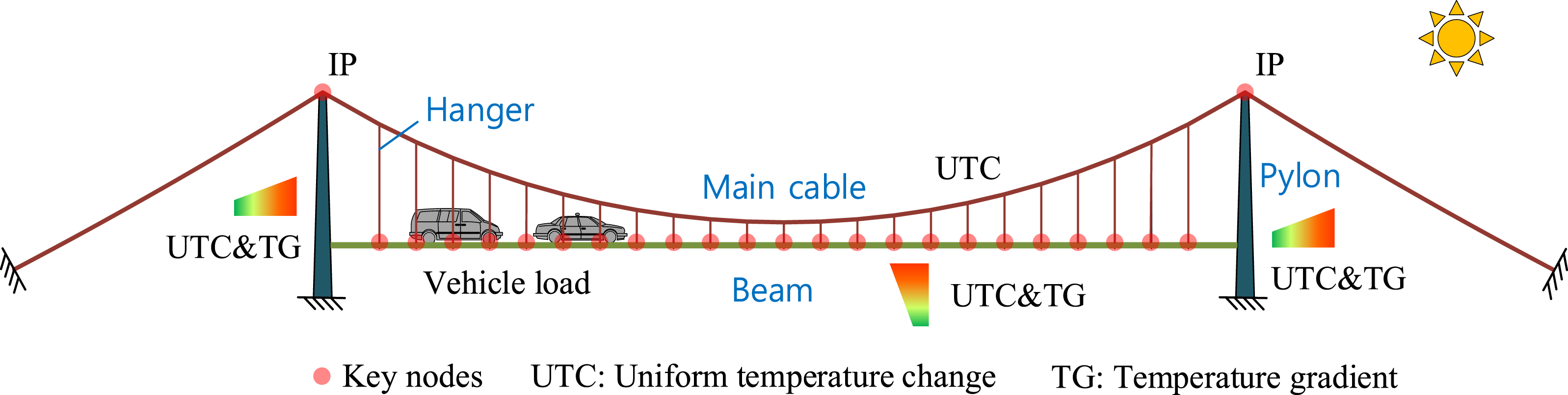

Before estimating the bridge response under the temperature-vehicle combined loading, all parameters and internal forces of each bridge component in the completed state are already known. That is, the lengths of each main cable segment and hangers, the internal forces of the main cable and hangers, and the vertical curve of the beam have already been obtained.

For convenience and simplicity, some less significant factors are neglected. The proposed analytical method is created based on the following assumptions:

(1) The main cable and hangers are ideally flexible cables only subject to tension. The main cable and hangers are free from compression, shear force, and bending moment at any position.

(2) The cable obeys Hooke’s law. Under both dead and live loads, its stresses and strains are linearly related.

(3) The temperature gradients in the beam and pylons are assumed to be linear. A length of uniformly distributed load simulates the vehicle load.

Although actual temperature distributions in bridge decks and pylons are often nonlinear due to environmental factors such as solar radiation, this does not affect the applicability of the proposed method. When necessary, the method can be extended to account for nonlinear temperature effects. For the sake of simplicity and clarity, a linear temperature gradient is assumed in this study.

Main cable

A Cartesian coordinate system and a Lagrangian coordinate system are built at the IP of the main cable and the i^-th hanger, named O_i. The X-axis of the Cartesian coordinate system points horizontally to the right, and the Y-axis vertically downwards. The left end of the cable segment is subjected to a horizontal component of force H_i and a vertical component of force V_0,i. Consider a point D in the main cable. The Lagrangian coordinates of this point with and without the self-weight are denoted by s and p, respectively. Under self-weight, the Cartesian coordinates are denoted by (x, y). The schematic diagram of the stress state of the main cable is shown in Figure 2.

Figure 2.

Schematic diagram of the force on the i^-th section of the main cable.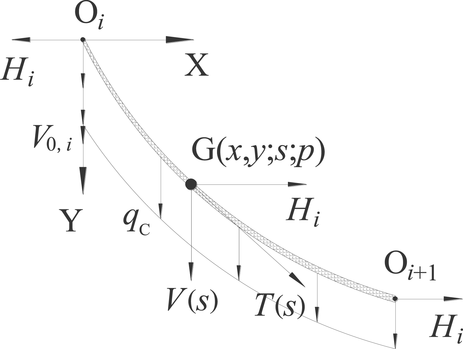

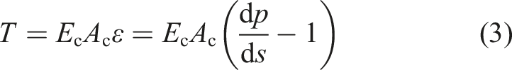
The internal force at point D can be obtained based on the conditions for force balance in the cable segment via equation (1) and the geometric compatibility via equation (2). Based on Hooke’s law, the tension T at point D can be expressed via equation (3).

V (s) = V_{0, i} - q_{c} s

(1)

T (s) = \sqrt{H_{i}^{2} + V {(s)}^{2}} = H_{i} \frac{d p}{d x} = V (s) \frac{d p}{d y}

(2)

T = E_{c} A_{c} ε = E_{c} A_{c} (\frac{d p}{d s} - 1)

(3)

where T and V are the tension and vertical force in the main cable, respectively; ε is the strain of the main cable under self-weight; E_c and A_c are the main cable’s elastic modulus and cross-sectional area, respectively.

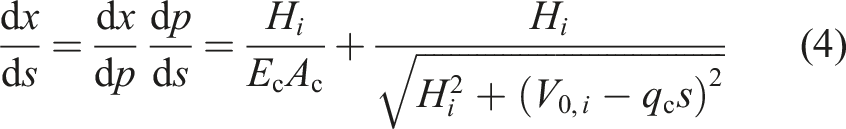
Based on equations (1)–(3), the differential relationship between the Cartesian coordinates (x, y) and the Lagrangian coordinate s can be represented by:

\frac{d x}{d s} = \frac{d x}{d p} \frac{d p}{d s} = \frac{H_{i}}{E_{c} A_{c}} + \frac{H_{i}}{\sqrt{H_{i}^{2} + {(V_{0, i} - q_{c} s)}^{2}}}

(4)

\frac{d y}{d s} = \frac{d y}{d p} \frac{d p}{d s} = \frac{V_{0, i} - q_{c} s}{E_{c} A_{c}} + \frac{V_{0, i} - q_{c} s}{\sqrt{H_{i}^{2} + {(V_{0, i} - q_{c} s)}^{2}}}

(5)

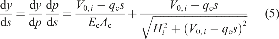
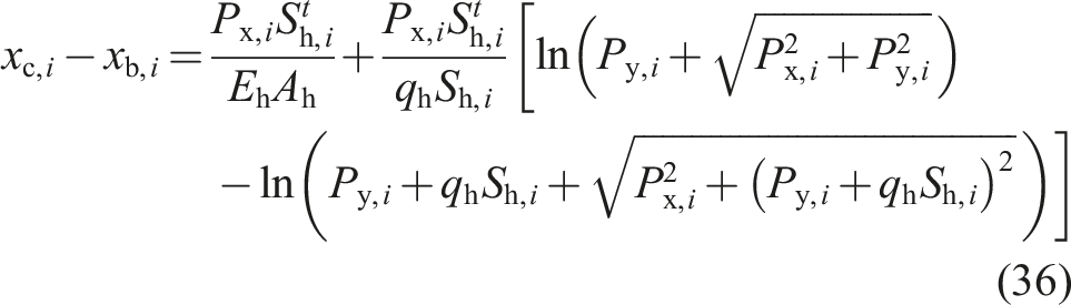
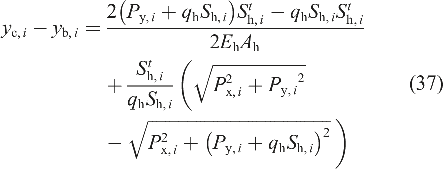
Integration is performed on the two sides of the equations (4) and (5) concerning s, and the boundary conditions of the main cable are introduced to solve the integration constant. The local coordinates at the right end of the main cable are derived via equations (6) and (7), becoming equal to the coordinate differences between the two ends of the i^-th main cable segment:

Δ x_{c, i} = \frac{H_{i} S_{c, i}}{E_{c} A_{c}} - \frac{H_{i}}{q_{c}} [\ln (V_{0, i} - q_{c} S_{c, i} + \sqrt{H_{i}^{2} + {(V_{0, i} - q_{c} S_{c, i})}^{2}}) - \ln (V_{0, i} + \sqrt{H_{i}^{2} + V_{0, i}^{2}})]

(6)

Δ y_{c, i} = \frac{2 V_{0, i} S_{c, i} - q_{c} S_{c, i}^{2}}{2 E_{c} A_{c}} + \frac{1}{q_{c}} (\sqrt{H_{i}^{2} + V_{0, i}^{2}} - \sqrt{H_{i}^{2} + {(V_{0, i} - q_{c} S_{c, i})}^{2}})

(7)

where Δx_c,i, Δy_c,i are the coordinate differences between the two ends of the i^-th main cable segment; S_c,i is the unstressed length of the i^-th main cable segment.

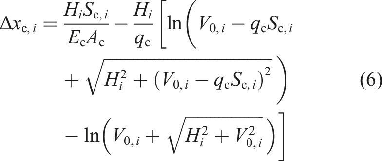
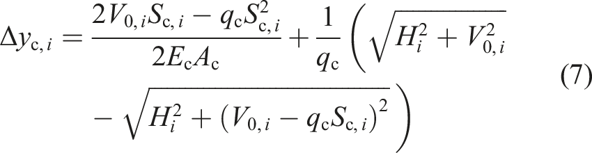
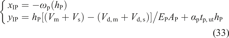
When the main cable is subjected to uniform temperature change t_c,ut, the expressions for the local coordinates at the right end of the main cable are given by:

Δ x_{c, i} = \frac{H_{i} S_{c, i}^{t}}{E_{c} A_{c}} - \frac{H_{i} S_{c, i}^{t}}{q_{c} S_{c, i}} [\ln (V_{0, i} - q_{c} S_{c, i} + \sqrt{H_{i}^{2} + {(V_{0, i} - q_{c} S_{c, i})}^{2}}) - \ln (V_{0, i} + \sqrt{H_{i}^{2} + V_{0, i}^{2}})]

(8)

Δ y_{c, i} = \frac{2 V_{0, i} S_{c, i}^{t} - q_{c} S_{c, i} S_{c, i}^{t}}{2 E_{c} A_{c}} + \frac{S_{c, i}^{t}}{q_{c} S_{c, i}} (\sqrt{H_{i}^{2} + V_{0, i}^{2}} - \sqrt{H_{i}^{2} + {(V_{0, i} - q_{c} S_{c, i})}^{2}})

(9)

S_{c, i}^{t} = (1 + α_{c} t_{c, ut}) S_{c, i}

(10)

where

S_{c, i}^{t}

is the unstressed length of the i^-th main cable segment under the thermal load; α_c is the coefficient of linear expansion of the main cable.

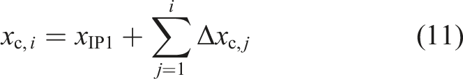
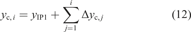
Hence, the coordinates x_c,i and y_c,i of the point where the i^-th hanger intersects with the main cable are given by:

x_{c, i} = x_{IP 1} + \sum_{j = 1}^{i} Δ x_{c, j}

(11)

y_{c, i} = y_{IP 1} + \sum_{j = 1}^{i} Δ y_{c, j}

(12)

where x_IP1 and y_IP1 are coordinates of the IP1 point, respectively.

According to the force balance in the main cable and at the anchor point of the hanger and the overall stress balance in the i^-th main cable segment, the recurrence relation of the internal force of the main cable is expressed by:

V_{0, i + 1} = V_{0, i} - (P_{y, i} + q_{h} S_{h . i}) - q_{c} S_{c, i}

(13)

H_{i + 1} = H_{i} + P_{x, i}

(14)

where P_x,i and P_y,i are the components of tension at the hanger bottom along the X- and Y-axes under the loading, respectively; q_h is the self-weight of the hanger per linear meter; S_h,i is the unstressed length of the i^-th hanger.

As shown above, the basic unknown parameters involved in the main cable calculation are the coordinates of the left IP under the temperature-vehicle combined loading, hanger tension, and the main cable tension at the left IP.

Beam

Under the live load, the beam is subject to the combined action of gravity q_g, hanger tension P, vehicle load p, and thermal load (uniform temperature change t_g,ut and temperature gradient t_b,tg). The positive directions of each variable are defined as follows: the upward displacement of the beam is considered positive; the bending moment causing tension in the upper surface and compression in the lower surface of the beam is considered positive; the downward force is considered positive.

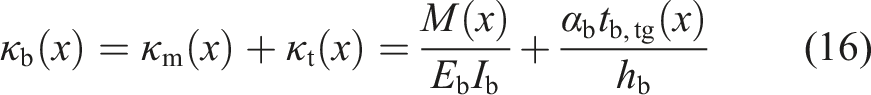
The bending moment, curvature, rotational angle, and deflection of the beam are represented by equations (15)–(18), respectively.

M_{b} (x) = M_{H} (x) + M_{L} (x) + M_{G} (x)

(15)

κ_{b} (x) = κ_{m} (x) + κ_{t} (x) = \frac{M (x)}{E_{b} I_{b}} + \frac{α_{b} t_{b, tg} (x)}{h_{b}}

(16)

θ_{b} (x) = \int κ (x) = \int [\frac{M (x)}{E_{b} I_{b}} + \frac{α_{b} t_{b, tg} (x)}{h_{b}}]

(17)

ω_{b} (x) = \iint κ (x) = \iint [\frac{M (x)}{E_{b} I_{b}} + \frac{α_{b} t_{b, tg} (x)}{h_{b}}]

(18)

where E_b and I_b are the elastic modulus and the cross-sectional moment of inertia of the beam, respectively; α_b is the coefficient of linear expansion of the beam; h_b is the beam height.

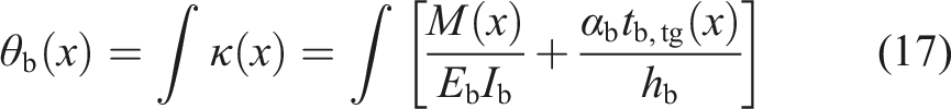
The integration constants contained in the deflection expression are solved based on the continuity conditions for the beam at the hanger’s site and the beam’s boundary conditions. The integration constants obtained by the solving process are introduced into the deflection expression to estimate the vertical deformation of the beam under the temperature-vehicle combined loading.

Assuming that the vehicle load is equivalent to a length multiplied by the uniformly distributed load, as shown in Figure 3, equation (19) expresses the beam’s bending moment:

M_{b} (x) = {\begin{cases} - \sum_{j = 0}^{i - 1} P_{y, j} (x - x_{b, j}) + \frac{1}{2} q_{b} x^{2}, x_{b, i - 1} \leq x < x_{b, i} \cap x < x_{L 1} \\ - \sum_{j = 0}^{i - 1} P_{y, j} (x - x_{b, j}) + \frac{1}{2} p {(x - x_{L 1})}^{2} + \frac{1}{2} q_{b} x^{2}, x_{b, i - 1} \leq x < x_{b, i} \cap x_{L 1} \leq x < x_{L 2} \\ - \sum_{j = 0}^{i - 1} P_{y, j} (x - x_{b, j}) + \frac{1}{2} p [{(x - x_{L 1})}^{2} - {(x - x_{L 2})}^{2}] + \frac{1}{2} q_{b} x^{2}, x_{b, i - 1} \leq x < x_{b, i} \cap x \geq x_{L 2} \end{cases}

(19)

Figure 3.

Schematic diagram of the force acting on the main beam (P_y,0 and P_y,n+1 are the vertical forces offered by the two pylons).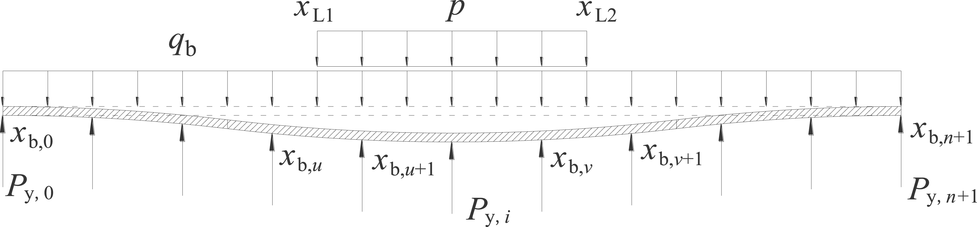

It has been generally agreed that the temperature field in the beam varies little along the length of the bridge. If the variation of the beam temperature along the bridge is neglected, the inclination angle and the defection of the beam can be calculated via equations (20)–(23).

ω_{b} (x) = {\begin{cases} D_{1} (x) + D_{2} (x) + C_{1, i} x + C_{2, i}, x_{b, i - 1} \leq x < x_{b, i} \cap x < x_{L 1} \\ \frac{p {(x - x_{L 1})}^{4}}{24 E_{b} I_{b}} + D_{1} (x) + D_{2} (x) + C_{3, i} x + C_{4, i}, x_{b, i - 1} \leq x < x_{b, i} \cap x_{L 1} \leq x < x_{L 1} \\ \frac{p {(x - x_{L 1})}^{4}}{24 E_{b} I_{b}} - \frac{p {(x - x_{L 2})}^{4}}{24 E_{b} I_{b}} + D_{1} (x) + D_{2} (x) + C_{5, i} x + C_{6, i}, x_{b, i - 1} \leq x < x_{b, i} \cap x \geq x_{L 2} \end{cases}

(20)

D_{1} (x) = - \frac{1}{E_{b} I_{b}} \sum_{j = 0}^{i - 1} P_{y, j} (\frac{x^{3}}{6} - \frac{x_{b, j}}{2} x^{2}), D_{2} (x) = \frac{q_{b} x^{4}}{24 E_{b} I_{b}} + \frac{α_{b} t_{b, tg}}{2 h_{b}} x^{2}

(21)

θ_{b} (x) = {\begin{cases} D_{3} (x) + D_{4} (x) + C_{1, i}, x_{b, i - 1} \leq x < x_{b, i} \cap x < x_{L 1} \\ \frac{p {(x - x_{L 1})}^{3}}{6 E_{b} I_{b}} + D_{3} (x) + D_{4} (x) + C_{3, i}, x_{b, i - 1} \leq x < x_{b, i} \cap x_{L 1} \leq x < x_{L 2} \\ \frac{p {(x - x_{L 1})}^{3}}{6 E_{b} I_{b}} - \frac{p {(x - x_{L 2})}^{3}}{6 E_{b} I_{b}} + D_{3} (x) + D_{4} (x) + C_{5, i}, x_{b, i - 1} \leq x < x_{b, i} \cap x \geq x_{L 2} \end{cases}

(22)

D_{3} (x) = - \frac{1}{E_{b} I_{b}} \sum_{j = 0}^{i - 1} P_{y, j} (\frac{x^{2}}{2} - x_{b, j} x), D_{4} (x) = \frac{q_{b} x^{3}}{6 E_{b} I_{b}} + \frac{α_{b} t_{b, tg}}{h_{b}} x

(23)

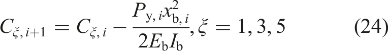
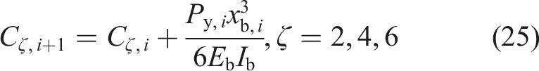
According to the continuity condition of the beam at x_b,i, we derive the recurrence relation between the integration constants.

C_{ξ, i + 1} = C_{ξ, i} - \frac{P_{y, i} x_{b, i}^{2}}{2 E_{b} I_{b}}, ξ = 1, 3, 5

(24)

C_{ζ, i + 1} = C_{ζ, i} + \frac{P_{y, i} x_{b, i}^{3}}{6 E_{b} I_{b}}, ζ = 2, 4, 6

(25)

By introducing the boundary conditions for the main beam and the continuity conditions for the vehicle load boundary, we can solve all of the integration constants.

C_{ξ, 1} = \frac{1}{6 E_{b} I_{b} x_{b, n + 1}} \sum_{j = 0}^{n} {P_{y, j} (x_{b, n + 1} - x_{b, j})}^{3} - \frac{p {(x_{b, n + 1} - x_{L 1})}^{4}}{24 E_{b} I_{b} x_{b, n + 1}} + \frac{p {(x_{b, n + 1} - x_{L 2})}^{4}}{24 E_{b} I_{b} x_{b, n + 1}} - \frac{q_{b} x_{b, n + 1}^{3}}{24 E_{b} I_{b}} - \frac{α_{b} t_{b, t g}}{2 h_{b}} x_{b, n + 1}, ξ = 1, 3, 5

(26)

C_{ζ, 1} = 0, ζ = 2, 4, 6

(27)

The integration constants thus calculated are introduced into the expressions of beam deflection and inclination angle to obtain the vertical deformation of the beam under the temperature-vehicle combined loading. The pier deformation is very small, so it has been omitted from the calculation.

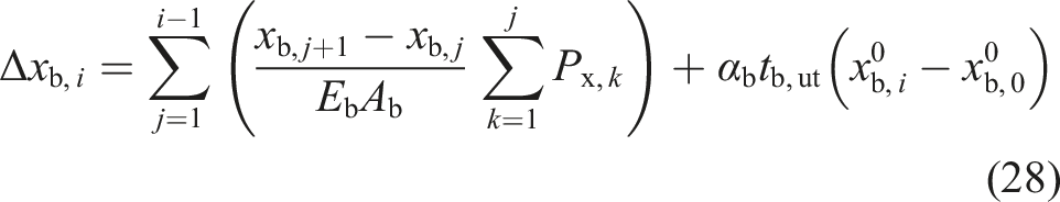
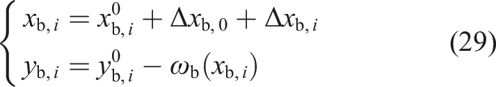
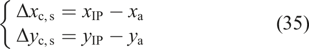
Since the stiffness of the expansion joint is far smaller than that of the beam, the beam undergoes an overall displacement under the live load. Using the left end of the beam as the benchmark, the relative displacement Δx_b,i of the anchor point of the i^-th hanger in the beam along the X-axis is expressed by:

Δ x_{b, i} = \sum_{j = 1}^{i - 1} (\frac{x_{b, j + 1} - x_{b, j}}{E_{b} A_{b}} \sum_{k = 1}^{j} P_{x, k}) + α_{b} t_{b, ut} (x_{b, i}^{0} - x_{b, 0}^{0})

(28)

Finally, under the temperature-vehicle combined loading, the coordinates (x_b,i, y_b,i) of the i^-th IP of the hanger and the beam are given by:

{\begin{cases} x_{b, i} = x_{b, i}^{0} + Δ x_{b, 0} + Δ x_{b, i} \\ y_{b, i} = y_{b, i}^{0} - ω_{b} (x_{b, i}) \end{cases}

(29)

where (

x_{b, i}^{0}

y_{b, i}^{0}

) are the coordinates of the i^-th IP of the hanger and the beam under the dead load; Δx_b,0 is the displacement of the left beam end.

Notably, the derivation can be done similarly for other loading patterns, such as multiple concentrated forces. That is, the beam deformation under the temperature-vehicle combined loading can be estimated by introducing the differential relation between the internal force and the deformation of the beam, boundary conditions for the beam, and continuity conditions for the beam.

Pylon

In the completed state, the horizontal components of cable tension are equal in the main and side spans, and the pylons are subject to axial compression. Increasing the elevation at the top of the pylon during concrete pouring can easily remove the influence of the huge axial pressure. However, when the bridge is subject to the vehicle load, the main cable on the two sides of the pylon is subject to an imbalance of horizontal components of hanger force, thus inducing pylon bending. Furthermore, the temperature gradient in the pylon can also cause its deformation. As a result, the enormous vertical pressure acting on the pylon generates a new bending moment. That is, the pylon undergoes a significant P-delta effect. The above-described influence factor must be considered when calculating the displacement of the IP under the temperature-vehicle combined effect.

The stress state of the pylon under the temperature-vehicle combined loading is shown in Figure 1. The top of the pylon is subject to unbalanced horizontal components of force and vertical force exerted by the main cable. The pylon has uniform temperature changes t_p,ut and temperature gradients t_p,tg along the direction of the bridge length. A Cartesian coordinate system is built at the top of the deformation pylon as the origin, and the directions of its axes are shown in Figure 4.

Figure 4.

Force diagram of pylons under the temperature-vehicle combined loading.

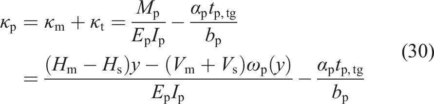
Suppose that the temperature gradient over the pylon cross-section is linear. Therefore, the curvature κ_p at any position in the pylon is composed of two parts, one induced by the bending moment and the other by the temperature gradient.

κ_{p} = κ_{m} + κ_{t} = \frac{M_{p}}{E_{p} I_{p}} - \frac{α_{p} t_{p, tg}}{b_{p}} = \frac{(H_{m} - H_{s}) y - (V_{m} + V_{s}) ω_{p} (y)}{E_{p} I_{p}} - \frac{α_{p} t_{p, tg}}{b_{p}}

(30)

where E_p, α_p, and I_p are the elastic modulus, coefficient of linear expansion, and bending moment of inertia, respectively; M_p is the bending moment; b_p is the dimension of the pylon along the bridge length direction.

Double integration is performed on the two sides of the above equation, and the pylon boundary conditions are introduced. So far, the expression of the pylon deformation under the temperature-vehicle combined loading can expressed by:

ω_{p} (y) = {D_{6}}^{- 3} [\begin{array}{l} \frac{α_{p} t_{p, tg}}{b_{P}} E_{p} I_{p} D_{6} \sin (D_{5} y) \tan (D_{5} h_{p}) - \frac{α_{p} t_{p, tg}}{b_{p}} E_{p} I_{p} D_{6} + (H_{m} - H_{s}) D_{6} y \\ + \frac{α_{p} t_{p, tg}}{b_{p}} E_{p} I_{p} D_{6} \cos (D_{5} y) - (H_{m} - H_{s}) \sqrt{E_{p} I_{p}} \sec (D_{5} h_{p}) \sin (D_{5} y) \end{array}]

(31)

D_{5} = \sqrt{\frac{V_{m} + V_{s}}{E_{P} I_{P}}}, D_{6} = \sqrt{V_{m} + V_{s}}

(32)

In the global coordinate system, the displacement of the pylon vertex (

x_{IP}

y_{IP}

) is given by:

{\begin{cases} x_{IP} = - ω_{p} (h_{P}) \\ y_{IP} = h_{P} [(V_{m} + V_{s}) - (V_{d, m} + V_{d, s})] / E_{P} A_{P} + α_{p} t_{p, ut} h_{P} \end{cases}

(33)

where V_d,m and V_d,s are the vertical components of main cable force in the main and side spans in the completed state, respectively; h_p and A_p are the height and cross-sectional area of the pylon, respectively.

Constraint conditions and optimization solutions

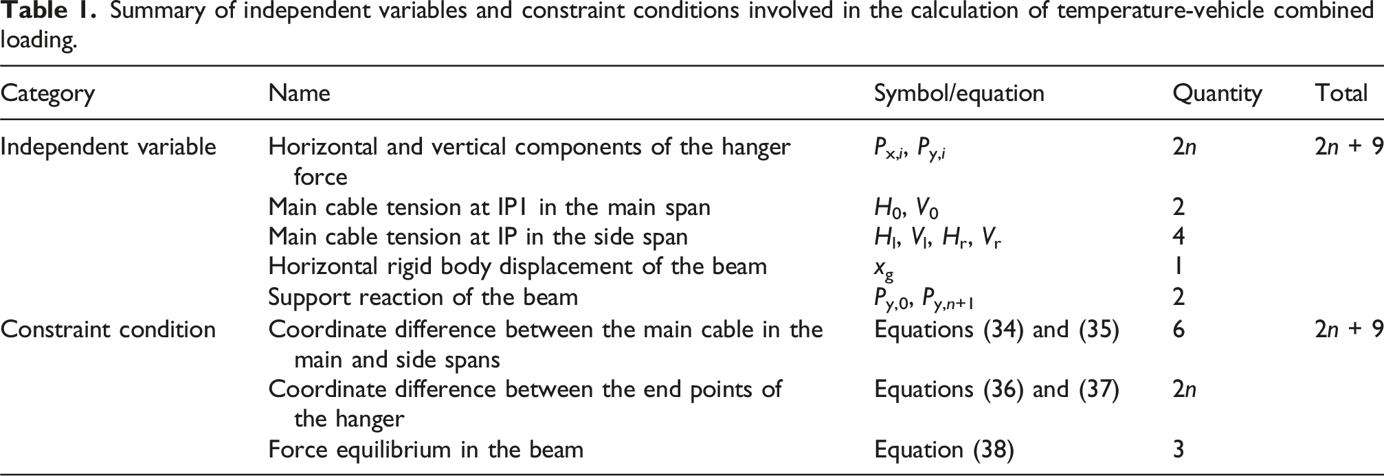
The computational derivation for each part of the suspension bridge under the temperature-vehicle combined loading in sections 2.2 to 2.4 is summarized. There are a total of 2n + 9 independent variables in the response calculation of the suspension bridge, including hanger force, main cable force, coordinates of IP, overall displacement of the beam along the bridge length direction, and support reaction of the pier. An equal number of constraint conditions are needed to solve these independent variables. Below, the details of each constraint condition are introduced.

The sum of the projected lengths of each main cable segment in the main span on the X- and Y-axes should be equal to the coordinate differences between the tops of the left and right pylons:

{\begin{cases} \sum_{i = 1}^{n + 1} Δ x_{c, i} = x_{IP 2} - x_{IP 1} \\ \sum_{i = 1}^{n + 1} Δ y_{c, i} = y_{IP 2} - y_{IP 1} \end{cases}

(34)

The sum of the projected lengths of each main cable segment in the side span on the X- and Y-axes should be equal to the coordinate differences between the top of the pylon and the anchor point in the main cable:

{\begin{cases} Δ x_{c, s} = x_{IP} - x_{a} \\ Δ y_{c, s} = y_{IP} - y_{a} \end{cases}

(35)

where Δx_c,s and Δy_c,s are the projected lengths of the main cable segment in the side span on the X- and Y-axes, respectively. Their expressions are the same as those for the main cable segments in the main span via equations (8) to (10).

The projected lengths of the hangers on the X- and Y-axes should equal the coordinate differences between the anchor points of the main cable and the main beam as follows:

x_{c, i} - x_{b, i} = \frac{P_{x, i} S_{h, i}^{t}}{E_{h} A_{h}} + \frac{P_{x, i} S_{h, i}^{t}}{q_{h} S_{h, i}} [\ln (P_{y, i} + \sqrt{P_{x, i}^{2} + P_{y, i}^{2}}) - \ln (P_{y, i} + q_{h} S_{h, i} + \sqrt{P_{x, i}^{2} + {(P_{y, i} + q_{h} S_{h, i})}^{2}})]

(36)

y_{c, i} - y_{b, i} = \frac{2 (P_{y, i} + q_{h} S_{h, i}) S_{h, i}^{t} - q_{h} S_{h, i} S_{h, i}^{t}}{2 E_{h} A_{h}} + \frac{S_{h, i}^{t}}{q_{h} S_{h, i}} (\sqrt{P_{x, i}^{2} + {P_{y, i}}^{2}} - \sqrt{P_{x, i}^{2} + {(P_{y, i} + q_{h} S_{h, i})}^{2}})

(37)

where Δx_h,i and Δy_h,i are the projected lengths of the i^-th hanger on the X- and Y-axes, respectively;

S_{h, i}

and

S_{h, i}^{t}

are the unstressed lengths of the i^-th hanger in the completed state of the bridge and after the uniform temperature change; α_h is the coefficient of linear expansion of the hanger; t_h,ut is the uniform temperature change of the hanger; E_h and A_h are the elastic modulus and cross-sectional area of the hanger, respectively.

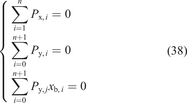
Since the stiffness of the expansion joint is far smaller than that of the beam, the constraint of the beam in the longitudinal direction of the bridge is neglected. Therefore, the sum of the horizontal components of hanger tension should be zero to maintain the force balance in the longitudinal direction of the bridge. Besides, the support reaction and the vertical component of the cable tension should satisfy the vertical force balance in the beam and make the moment at the beam end zero:

{\begin{cases} \sum_{i = 1}^{n} P_{x, i} = 0 \\ \sum_{i = 0}^{n + 1} P_{y, i} = 0 \\ \sum_{i = 0}^{n + 1} P_{y, j} x_{b, i} = 0 \end{cases}

(38)

Table 1 lists the independent variables, constraint conditions involved in the calculation, and their quantities.

Table 1.

Summary of independent variables and constraint conditions involved in the calculation of temperature-vehicle combined loading.

Category	Name	Symbol/equation	Quantity	Total
Independent variable	Horizontal and vertical components of the hanger force	P_x,i, P_y,i	2n	2n + 9
	Main cable tension at IP1 in the main span	H₀, V₀	2
	Main cable tension at IP in the side span	H_l, V_l, H_r, V_r	4
	Horizontal rigid body displacement of the beam	x _g	1
	Support reaction of the beam	P_y,0, P_y,n+1	2
Constraint condition	Coordinate difference between the main cable in the main and side spans	Equations (34) and (35)	6	2n + 9
	Coordinate difference between the end points of the hanger	Equations (36) and (37)	2n
	Force equilibrium in the beam	Equation (38)	3

Considering the high complexity and non-linearity of the system of equations for solving the response of the suspension bridge, it is almost impossible to solve the analytical expressions of each independent variable directly. It will be far more efficient to convert equation-solving into an optimization problem. The constraint condition, that is, the square of differences on the two sides of equations (35)–(38), is treated as an optimization term, and the sum of all optimization terms is considered the overall optimization objective 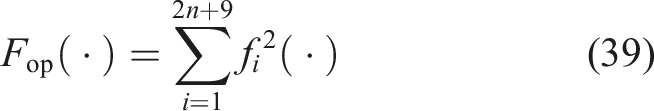$F_{op} (\cdot)$ . Next, the generalized reduced gradient method (GRG) is employed to solve the problem and obtain the response of the suspension bridge under the temperature-vehicle combined loading.

F_{op} (\cdot) = \sum_{i = 1}^{2 n + 9} {f_{i}}^{2} (\cdot)

(39)

where

f_{i} (\cdot)

is the i^-th optimization term.

Briefly, the proposed method consists of the following steps:

Step 1: Initialize the independent variables that are listed in Table 1;

Step 2: Calculate the deformations of the main cable, pylons, and beam separately. The equations used for the above purpose are equations (8)–(12), equations (19)–(29), and equations (31)–(33);

Step 3: Calculate the residuals of constraint equations based on the displacements of key nodes under the live load. The constraint equations involved are equations (34)–(38);

Step 4: Treat the residual sum of squares of the constraint equations as the optimization objective F_op(·). The GRG method is employed to iteratively adjust the independent variables and minimize F_op(·). In each iteration, the GRG method calculates the gradient of the objective function, determines the optimal search direction, and updates the independent variables accordingly. The process continues until F_op(·) no longer changes significantly or meets the convergence conditions.

Convergence Criteria: The maximum iteration number is set to 20, and the convergence threshold is set to 1 × 10⁻¹⁵. The solution is considered converged when the residual sum of squares falls below this threshold. This setting has shown good convergence and stability in numerical examples.

The following figure shows the calculation flow chart (Figure 5).

Figure 5.

Flow chart of the analytical method for suspension bridge response under temperature-vehicle combined loading.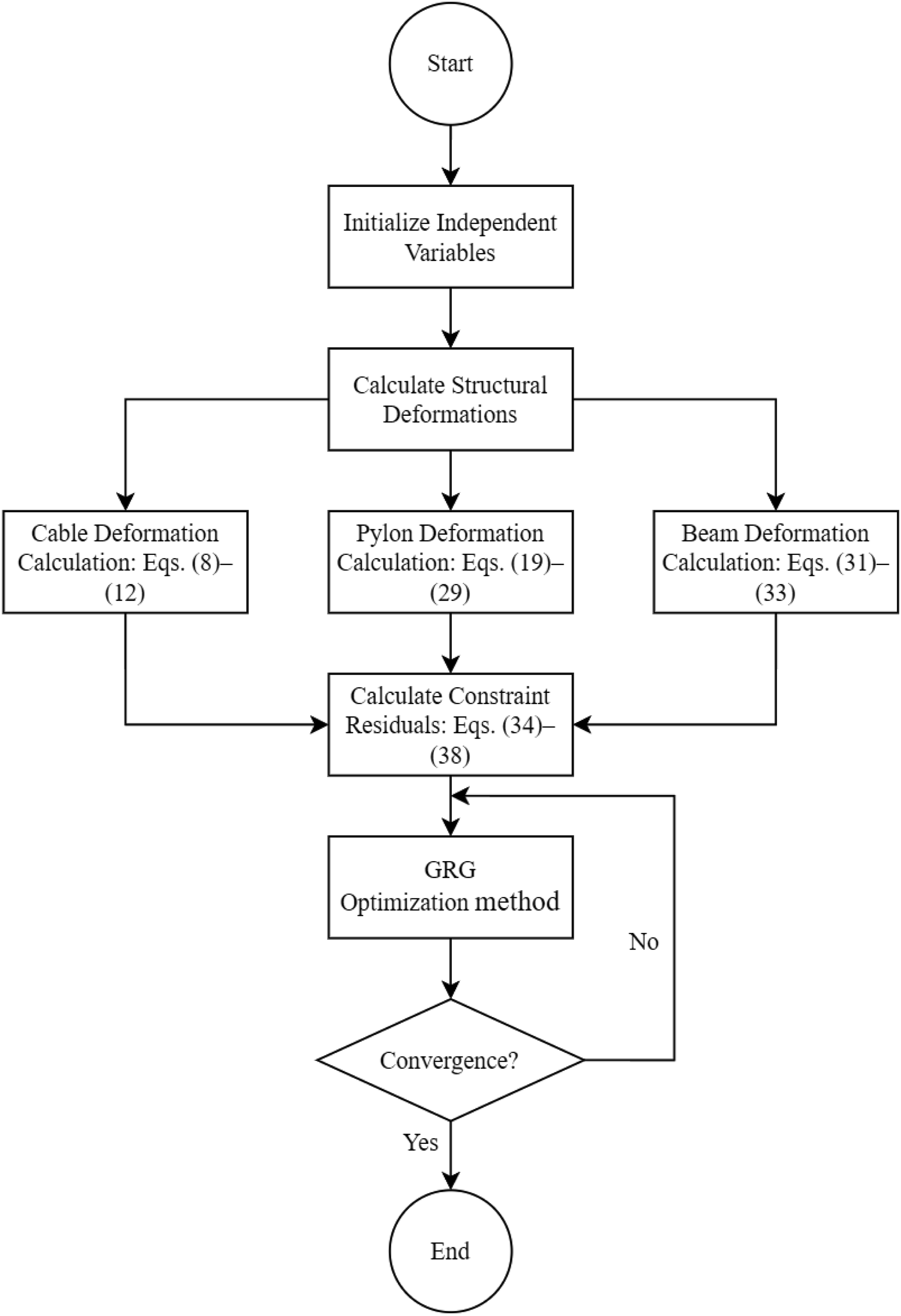

The subsequent case study indicates that when the initial values of all independent variables are set to be equal to those in the completed state of the bridge (that is, the live load response is set to 0), a fast convergence is achieved for the optimization. This has demonstrated the proposed method’s excellent convergence performance and numerical computational efficiency.

Numerical example

Bridge layout and structural parameters

A numerical example of a suspension bridge with a main span of 1700 m is used to verify the effectiveness and accuracy of the proposed method. The span length layout is 465 m + 1700 m + 465 m. There are 93 hangers in the main span, spaced 18 m apart. The horizontal distance from the first hanger to the IP in the main cable is 22 m. The rise-span ratio of the main cable is 1/9. The width and height of the stiffening beam are 28 m and 10 m, respectively.

Regarding the traffic load, the upper deck has six roadways, and the lower deck has a double-track railway. The lane load of roadways and railways are respectively assumed to 10.5 kN/m and 40 kN/m based on the Chinese bridge standards. The reduction factor of roadways is set to 0.6. The overall uniformly distributed load of 100 kN/m is applied. Two load distribution patterns are considered: uniform load acting for left half of the span length and uniform load acting for 1/4 to 3/4 of the span length.

As to the thermal load, the overall uniform temperature change is set to ±30°C for the bridge based on the measured data from the SHM system of the Yangsigang Bridge. Temperature gradients of 20°C, 10°C, and 30°C are imposed on the left pylon, right pylon, and stiffening beam, respectively.

The elevation layout of the suspension bridge and the load distribution pattern are shown in Figure 6. The structural parameters and the temperature load acting on the suspension bridge are shown in Table 2. The load distribution parameters for each load condition are shown in Table 3.

Figure 6.

Elevation layout of the suspension bridge and loading.

Table 2.

Bridge parameters and thermal load.

Bridge parameter (unit)	Value	Bridge parameter (unit)	Value
Elastic modulus of the main cable (kPa)	2 × 10⁸	Pylon height (m)	231.9
Self-weight of the main cable per meter (kN/m)	58.015	Pylon width in the longitudinal direction of the bridge (m)	14
Cross-sectional area of the main cable (m²)	0.744	The cross-sectional area of the pylon (m²)	69.84
Elastic modulus of the hanger (kPa)	1.1 × 10⁸	Elastic modulus of the beam (kPa)	2.05 × 10⁸
Self-weight of the hanger per meter (kN/m)	1.25832	Moment of inertia of the beam (m⁴)	117.11
The cross-sectional area of the hanger (m²)	1.6356 × 10^-2	The cross-sectional area of the beam (m²)	4.631
Elastic modulus of the pylon (kPa)	3.5 × 10⁷	Dead weight of the beam per linear meter (kN/m)	398.22
Moment of inertia of the pylon along the bridge length direction (m⁴)	1551.8	Coefficient of linear expansion	1.2 × 10⁻⁵

Table 3.

Load distributions under each case.

Case no.	Loading condition no.	Vehicle load (kN/m)	Range of loading	Overall temperature change	Temperature change in the beam	Temperature change in the left pylon	Temperature change in the right pylon
Case 1	Loading condition 1	100	Half span	+30°C	+30°C	+20°C	+10°C
Case 2	Loading condition 2	100	1/4–3/4 of the span	+30°C	+30°C	+20°C	+10°C
Case 3	Loading condition 3	100	Half span	−30°C	+30°C	+20°C	+10°C
Case 4	Loading condition 4	100	1/4-3/4 of the span	−30°C	+30°C	+20°C	+10°C

Completed state of suspension bridge

The shape-finding approaches for the main cable in the bridge’s completed state have already matured. In this study, we determine the cable shape of the suspension bridge in the completed state using the segmental catenary theory proposed by Zhang et al. (2023). Their method can be roughly described as follows:

(1) The hanger tension is calculated in the completed state of the bridge using the zero displacement method.

(2) Assume that the main cable shape between the adjacent hangers is a catenary via equation (40). Since the hangers remain vertical in the completed state of the bridge, the horizontal component of the main cable tension is constant. Let the shape parameter a_i of each main cable segment be a basic unknown parameter. The recurrence relation of a_i is obtained based on force equilibrium at each node of the main cable.

y = c_{i} [\cosh (\frac{x}{c_{i}} + a_{i}) - \cosh a_{i}]

(40)

where c_i = −H/q; q is the self-weight of the main cable per meter; a_i is the shape parameter of the i^-th catenary.

(3) The main cable’s rise-span ratio and the cable ends’ elevation, two known parameters, are used as constraints. The shape parameter a₁ of the first main cable segment and the horizontal component of force H in the main cable are calculated to find the main cable shape in the completed state.

(4) Once the main cable shape has been determined, the initial strain in each main cable segment can be estimated via:

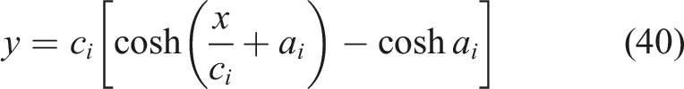
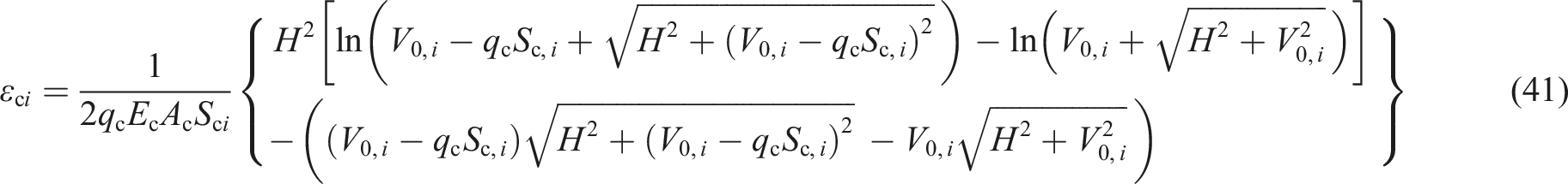
ε_{c i} = \frac{1}{2 q_{c} E_{c} A_{c} S_{c i}} {\begin{cases} H^{2} [\ln (V_{0, i} - q_{c} S_{c, i} + \sqrt{H^{2} + {(V_{0, i} - q_{c} S_{c, i})}^{2}}) - \ln (V_{0, i} + \sqrt{H^{2} + V_{0, i}^{2}})] \\ - ((V_{0, i} - q_{c} S_{c, i}) \sqrt{H^{2} + {(V_{0, i} - q_{c} S_{c, i})}^{2}} - V_{0, i} \sqrt{H^{2} + V_{0, i}^{2}}) \end{cases}}

(41)

Figure 7 shows the main cable shape and hanger tensions solved using different methods in the completed state of the bridge.

Figure 7.

Main cable shape and hanger tensions in the completed state of the bridge.

Finite element model

A finite element model of the suspension bridge is built using the ANSYS software. The entire bridge has 567 nodes and 754 elements. The pylons and beam are simulated with beam 188 elements while cable and hangers are simulated with link 180 elements. The material properties of these components, including elastic modulus, density, and coefficient of thermal expansion, were set according to Table 2. The beam deformation in the transverse direction of the bridge is neglected under the live load. The main beam and the pylon cross-beam are simulated using a fishbone beam model with a rigid arm. The density and the coefficient of linear expansion of the rigid arm are both 0, and the cross-sectional moment of inertia is 5000 m⁴. The splay saddle and the saddle on top of the pylon are omitted. The IP in the main cable and the top of the pylon share one common node.

As to the constraints, the main cable’s ends and the pier’s bottom are considered consolidated, and their displacements are fully constrained. The ends of the stiffening beam constrain the rotation in the normal directions, defined as the longitudinal and vertical directions of the bridge. During the solving process, the vertical displacement of the main beam endpoint and the cross-beam midpoint are set to be equal, simulating the support of the main beam.

Temperature loads were applied by assigning specific temperature values to the eight nodes of each BEAM188 element, allowing for the simulation of both uniform temperature changes and linear temperature gradients. Specifically, the main cable and hangers were subjected to a uniform temperature rise of 30°C, while the beam and pylons experienced a temperature gradient ranging from 15°C to 45°C. Vehicle loads were modeled as uniformly distributed loads applied to the beam elements, implemented by setting load values at the I and J ends of the elements.

Significant deformation and geometric non-linearity are considered in the solving process. The Newton-Raphson method was employed, with the ‘SSTIF’ option enabled to account for stress stiffness. Additionally, the ‘NLGEOM’ command was activated to account for large deformation effects, ensuring the accuracy of the simulation results.

The bridge deformations under the cases 1 and 2 are shown in Figure 8.

Figure 8.

Deformations in the finite element model under cases 1 (a) and 2 (b) (amplification factor of 10, unit: m).

Comparison of calculation results

Figures 9 and 10 illustrate displacements of the nodes in the main cable along the X- and Y-axes under different cases, respectively. With the full load acting for half of the span length, the maximum absolute error between the values solved by the analytical method and the finite element method is only 2 cm. The corresponding relative error is 0.73%, occurring near the 3/4 position of the span. With the full load acting for 1/4 to 3/4 of the span length, the maximum absolute error between the values solved by the analytical method and the finite element method is only 1.5 cm. The corresponding relative error is 1.63%, occurring near the 1/4 position of the span. The main cable shapes are compared between the cases 1 and 3 and between the cases 2 and 4. It is easy to see that uniform temperature change greatly impacts the main cable shape. That is, the response of the suspension bridge induced by the same vehicle load differs dramatically in different seasons.

Figure 9.

Main cable displacements in the X-axis under the temperature-vehicle combined loading.

Figure 10.

Main cable displacements in the Y-axis under the temperature-vehicle combined loading.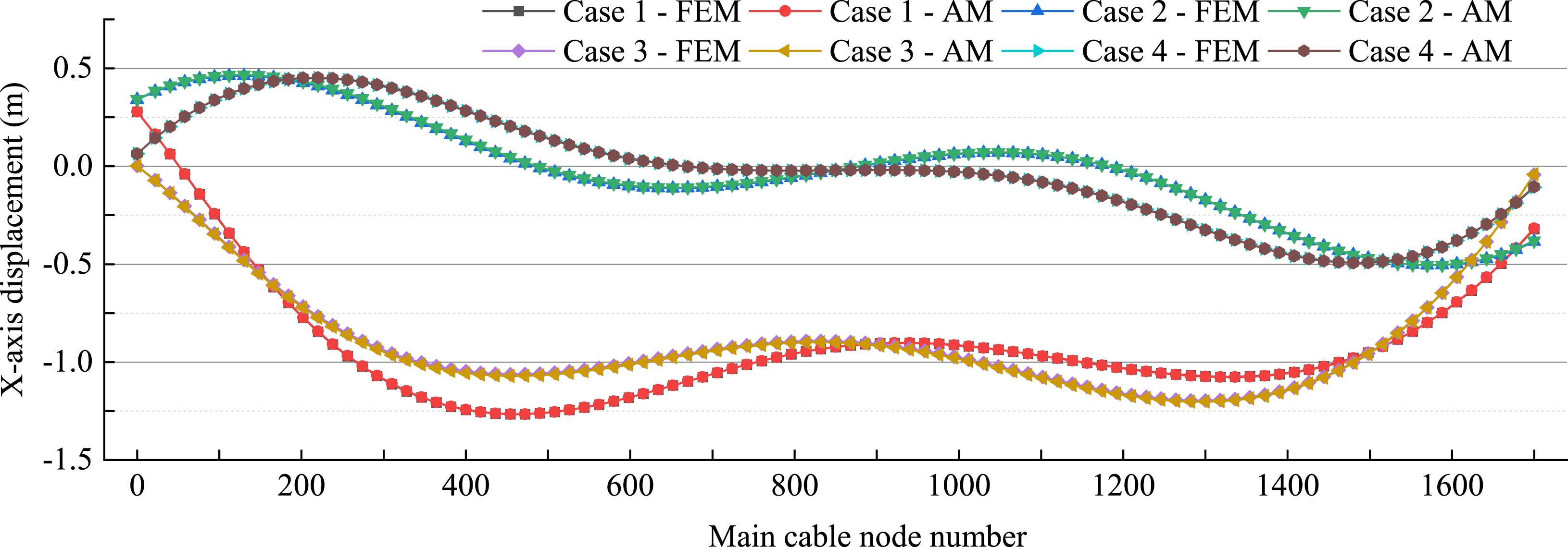

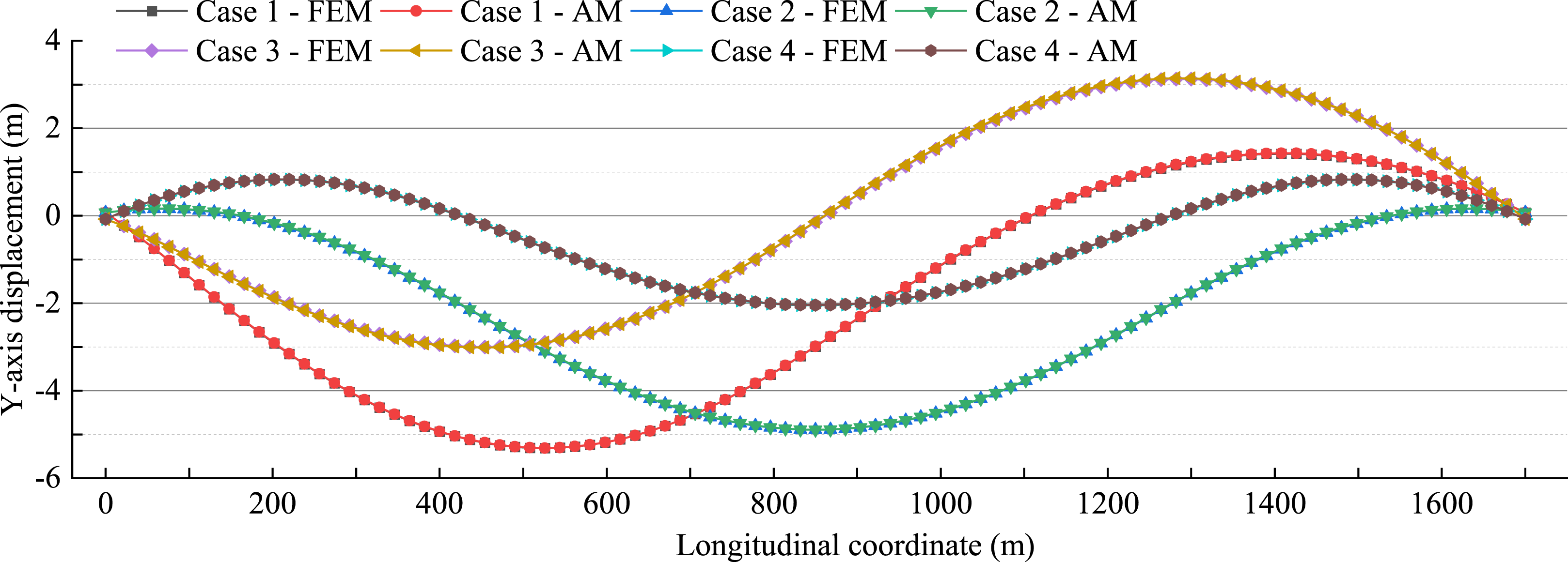
Figure 11 shows the variations of hanger tension with the temperature-vehicle combined loading acting on the bridge decks under cases 1 and 2. Under all cases, the maximum absolute error between the values solved by the finite element and analytical methods is less than 5 kN. Notably, under cases 1, 2, and 3, the variations of some hanger tensions near the pylons are negative. Especially under case 1, a change of −173.3 kN occurs to the tension in the first hanger from the left side with the uniform load acting on the left half-span, the largest negative increase among all cases. This finding contradicts our common belief about the changes in hanger tension under the live load but testifies to the significant impact of the thermal load on the response of the suspension bridge subject to the moving load.

Figure 11.

Variations in hanger forces under cases 1 and 2.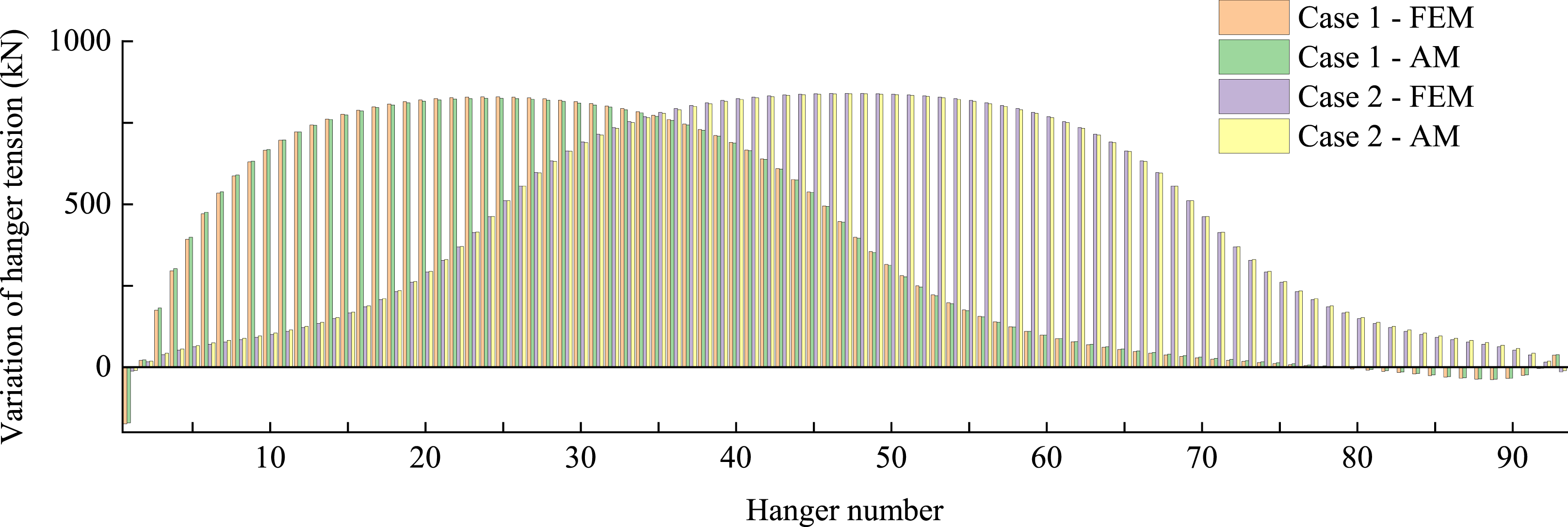

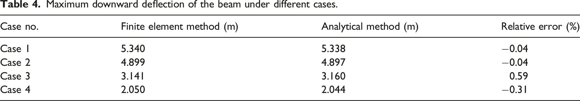
Tables 4 –6 summarize the maximum downward deflection, rotational angle of the beam end, and variation of the horizontal force component in the main cable, respectively. The above variables are the responses of the suspension bridge that draw the most attention from the engineers during live load design. The results show that except for the rotational angle of the beam end under case 2, where the relative error is too large due to an excessively small true value, the relative errors of the key responses of the suspension bridge under all cases are below 1%.

Table 4.

Maximum downward deflection of the beam under different cases.

Case no.	Finite element method (m)	Analytical method (m)	Relative error (%)
Case 1	5.340	5.338	−0.04
Case 2	4.899	4.897	−0.04
Case 3	3.141	3.160	0.59
Case 4	2.050	2.044	−0.31

Table 5.

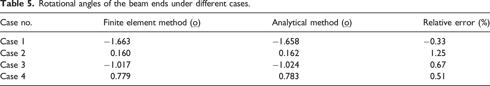
Rotational angles of the beam ends under different cases.

Case no.	Finite element method (º)	Analytical method (º)	Relative error (%)
Case 1	−1.663	−1.658	−0.33
Case 2	0.160	0.162	1.25
Case 3	−1.017	−1.024	0.67
Case 4	0.779	0.783	0.51

Table 6.

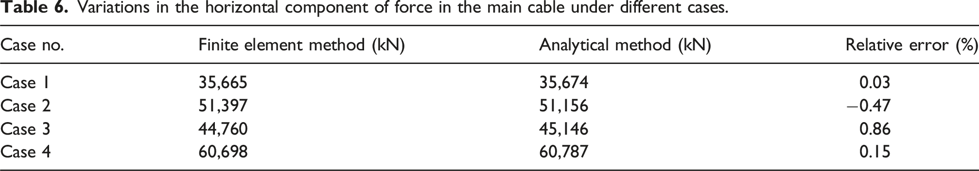
Variations in the horizontal component of force in the main cable under different cases.

Case no.	Finite element method (kN)	Analytical method (kN)	Relative error (%)
Case 1	35,665	35,674	0.03
Case 2	51,397	51,156	−0.47
Case 3	44,760	45,146	0.86
Case 4	60,698	60,787	0.15

The above results demonstrate the high accuracy of the proposed Analytical Method (AM) in calculating the response of the suspension bridge under the temperature-vehicle combined load.

Discussion

Coupling effects of the temperature and vehicle loads

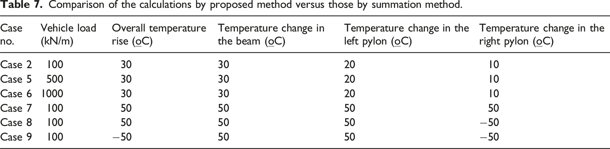
To analyze the coupling effect of the temperature and vehicle loads, cases 5–9 were developed based on case 2. The values of loads in each condition are displayed in Table 7. For each case, the proposed analytical method is employed to estimate the responses of the suspension bridge under the temperature-vehicle combined load, temperature -only, and vehicle -only. After that, a comparison is made between the results from the summation method (“temperature-only” plus “vehicle-only”) and the proposed method. The maximum beam deflection and rotational angle of the beam end are also compared yo meet the track smoothness requirement. The comparison of the calculations is shown in Table 8.

Table 7.

Comparison of the calculations by proposed method versus those by summation method.

Case no.	Vehicle load (kN/m)	Overall temperature rise (ºC)	Temperature change in the beam (ºC)	Temperature change in the left pylon (ºC)	Temperature change in the right pylon (ºC)
Case 2	100	30	30	20	10
Case 5	500	30	30	20	10
Case 6	1000	30	30	20	10
Case 7	100	50	50	50	50
Case 8	100	50	50	50	−50
Case 9	100	−50	50	50	−50

Table 8.

Comparison of the calculation results based on the coupling effects of temperature and vehicle loads versus those by simple summation.

Case no.	Maximum downward deflection of the beam			Rotational angle of the beam end
Case no.	Proposed method	Summation	Relative error (%)	Proposed method	Summation	Relative error (%)
Case 2	4.899	4.936	0.76	0.246	0.239	−2.97
Case 5	16.130	16.286	0.96	0.601	0.582	−3.16
Case 6	27.325	27.586	0.95	0.421	0.402	−4.42
Case 7	5.927	5.989	1.04	0.268	0.259	−3.47
Case 8	5.710	5.765	0.97	0.318	0.311	−2.30
Case 9	1.497	1.535	2.52	1.410	1.434	1.68

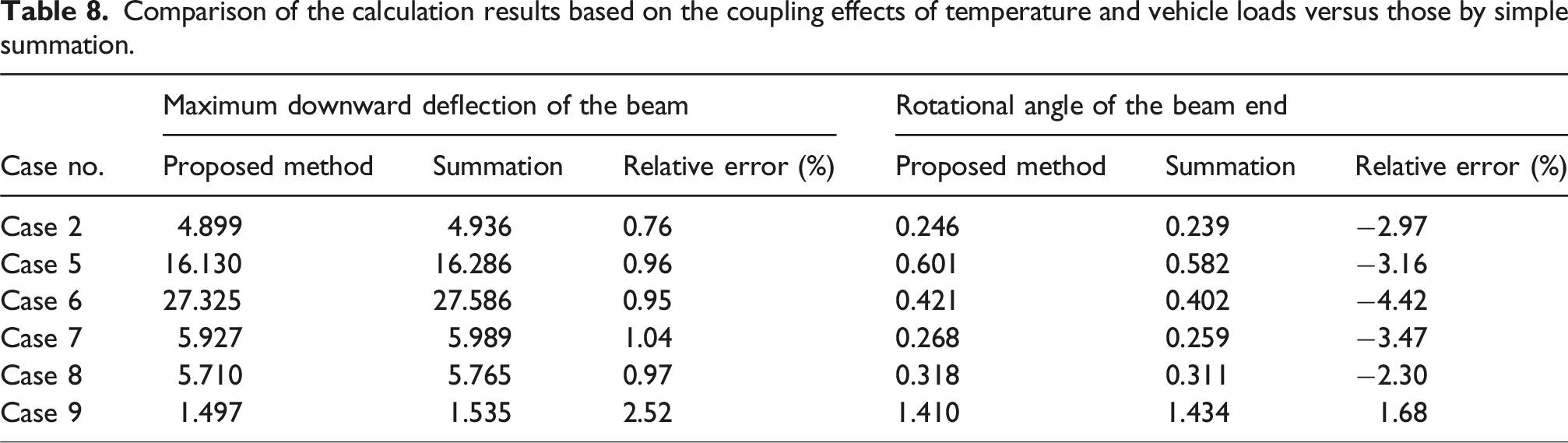
It can be inferred from the results in Table 8 that errors exist for the simple summation method, as compared to those from the proposed method. This is primarily due to the geometric non-linearity of the suspension bridge. The main cable deformation induced by thermal load will change the bending stiffness of the suspension bridge, which further affects the response of the suspension bridge under the vehicle load. The following phenomena are also observed:

(1) Under a normal live load, the coupling effect of the temperature and moving loads that induce the deformation is insignificant. For the maximum downward deflection of the beam and the rotational angle of the beam end, the relative errors between the two methods are 0.76% and −2.97%, respectively.

(2) As the vehicle load increases, the accuracy of the simple summation method in estimating the rotational angle of the beam end decreases. In this case study, when the vehicle load increases to 1000 kN/m, the relative error of the rotational angle of the beam end reaches −4.42%.

(3) Under the extreme thermal load, the coupling effect of the temperature and vehicle loads affects the accuracy of the simple summation method to a greater extent. Nevertheless, the magnitude of influence on the calculation results varies with different thermal load combinations, and no regular pattern is observed.

P-delta effect of the pylons

In a completed state of the bridge, the horizontal components of force are equal on the two sides of the pylon. The pylon is subject to axial compression. When there is a vertical temperature gradient in the pylon, the pylon will undergo deformation in the longitudinal direction of the bridge. Furthermore, the moving load on the beam makes the horizontal components of force in the main cable in the main span and the side spans no longer equal, which also causes the pylon to bend. The pylon deformation caused by loads plus the enormous vertical compression exerted by the main cable results in the P-delta effect, which greatly increases the displacement of the IP on the top of the pylon. However, most existing studies on the suspension bridge’s live load response do not consider the thermal load and the resulting deformation of the pylon. This may lead to an underestimation of the P-delta effect of the pylon and give rise to calculation errors. In this section, the calculation is performed under case 1 in section 3.1 without considering the P-delta effect of the pylon, and the results are compared.

Figure 12 shows the deformation with and without considering the P-delta effect of the pylon under case 1. It is found that neglecting the P-delta effect only incurs a small error in calculating the main cable deformation under case 1. Regarding the displacement along the X-axis, the maximum relative error is about 2.1% when the absolute value of the displacement is above 1 m. Regarding the displacement along the Y-axis, the maximum relative error is about 0.25% when the absolute value of the displacement is above 2 m. The above results may be explained by the fact that the P-delta effect of the pylon only has a very small impact on the main cable deformation, compared with the deformation caused by a uniform temperature rise of 30°C. It is worth noticing that the relative error for the displacement of the left IP in the main cable along the X-axis reaches 8.9%. This result indicates that neglecting the P-delta effect of the pylon gives rise to a significant error in calculating the pylon deformation.

Figure 12.

Comparison of the main cable deformation with and without considering the P-delta effect of the pylon: (a) X-axis; (b) Y-axis.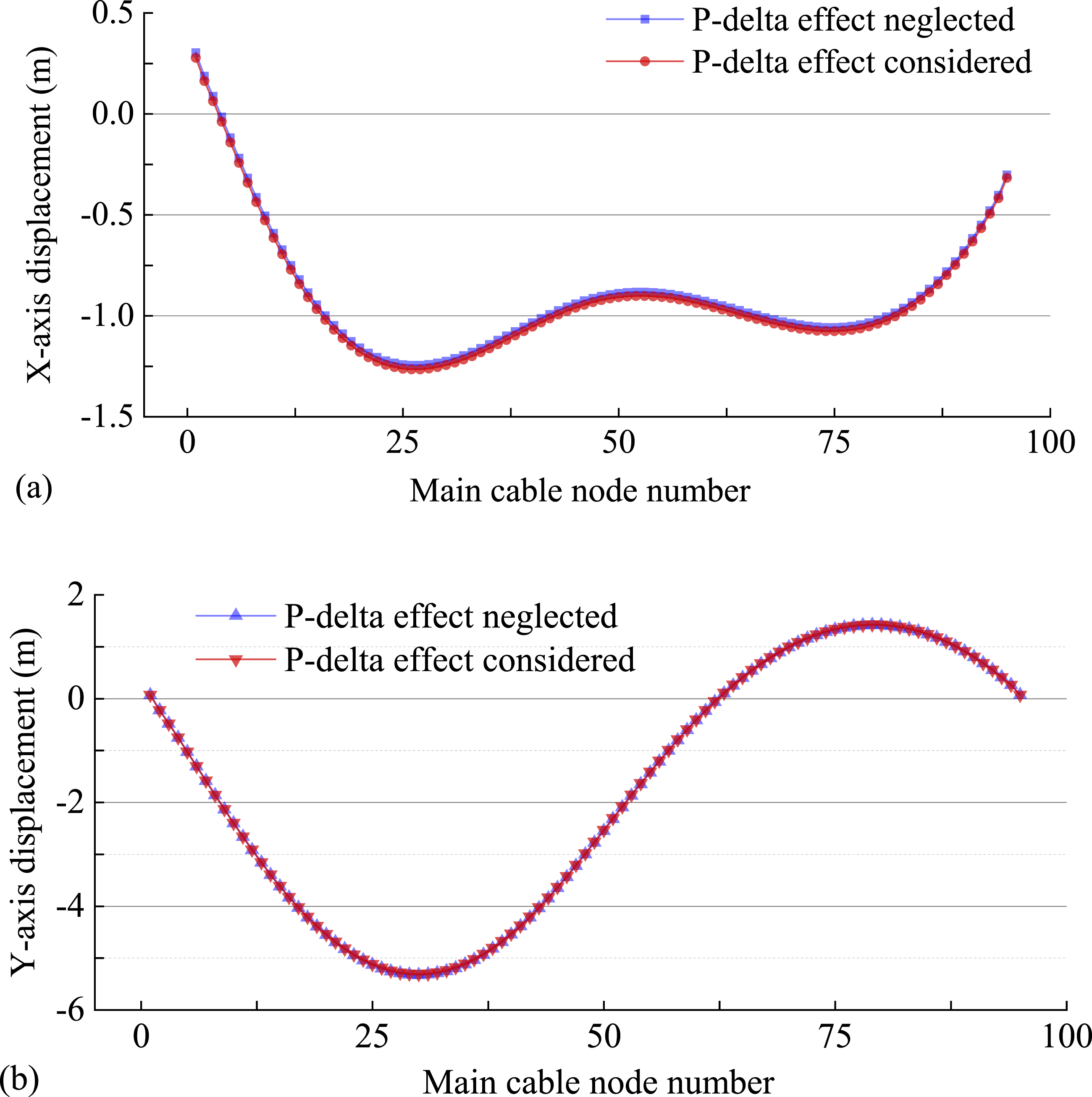

In addition, a peak phenomenon is observed in Figure 12(a), characterized by a reduced horizontal displacement of the central nodes of the main cable. This is primarily caused by the S-shaped deformation of the main beam under half-span loading, as shown in Figure 12(b). Due to the shorter hanger lengths and smaller vertical displacements of the main beam at mid-span, the negative horizontal displacement of the central nodes is restricted, resulting in the observed peak.

Conclusions

This study developed and verified an analytical method for solving the live load response of the suspension bridge. It features a clearly described derivation process and defines the physical meanings of all parameters involved. While most existing studies focus on the vehicle load, the proposed method considers how the thermal load contributes to the live load response of the suspension bridge. This method also considers the P-delta effect of the pylons. The convergence performance and calculation efficiency of the proposed method are verified through a numerical example. The following conclusions were drawn:

(1) The proposed method can precisely solve the response of the suspension bridge under the temperature-vehicle combined loading. It can consider multiple thermal loads and various distribution patterns of the moving load. For example, a suspension bridge with a main span of 1700 m has a maximum absolute error for beam deformation below 2 cm, proving the method’s accuracy.

(2) This approach comprehensively considers the suspension bridge’s geometric non-linearity while avoiding the iterative procedures in geometric non-linearity estimation. The case study offers convincing evidence about the high speed of convergence and the broadness of the convergence domain. In the case of a large suspension bridge with a main span of 1700 m, the programmed solving process only takes 1 min when the initial values of all basic known parameters are set to 0.

(3) Given the significant geometric non-linearity of the suspension bridge, the responses induced by the temperature and vehicle loads are combined. The coupling effect intensifies with increasing vehicle and temperature load levels, becoming significant under high loads, while the resulting calculation error is relatively small and negligible under typical loading conditions. For the vertical displacement of the main beam, the coupling effect has a minor influence. However, for sensitive indicators such as beam-end rotations, neglecting the coupling effect may lead to significant calculation errors. Therefore, whether the coupling effect can be ignored should be determined based on specific analysis objectives, load levels, and accuracy requirements.

(4) The P-delta effect of the pylon is mainly manifested as the deformation of the pylon during the live load response calculation of the suspension bridge. Under the uniform temperature rise of 30°C, vertical temperature gradient of 30°C in the beam, and temperature gradient of 20°C/10°C in the pylons, the relative error is only 2.1% for the main cable deformation if the P-delta effect of the pylon is neglected. However, the relative error of the calculated displacement of the IP in the main cable along the X-axis reaches 8.9%. The above results indicate the necessity of considering the pylon’s P-delta effect when analyzing the suspension bridge’s response under live loads.

(5) The proposed method primarily focuses on static analysis, while the effects of dynamic factors such as vehicle-induced vibrations, wind loads, and seismic actions remain to be explored. Additionally, to better align with engineering practice, additional factors such as non-uniform temperature gradients, material creep, and shrinkage could be incorporated into future research. Structural health monitoring data can also be utilized to validate the proposed method.

Footnotes

ORCID iD

Wen-ming Zhang

Funding

The authors disclosed receipt of the following financial support for the research, authorship, and/or publication of this article: The work described in this paper was financially supported by the National Key R&D Program of China (No. 2022YFB3706703), the National Natural Science Foundation of China under Grant Nos. 52078134 and 52378138, and the Fundamental Research Funds for the Central Universities, which are gratefully acknowledged.

Declaration of conflicting interests

The authors declared no potential conflicts of interest with respect to the research, authorship, and/or publication of this article.

References

Choi

Gwon

Yoo

, et al. (2013) Nonlinear static analysis of continuous multi-span suspension bridges. International Journal of Steel Structures 13(1): 103–115.

Choi

Gwon

(2014) Simplified analysis for preliminary design of towers in suspension bridges. Journal of Bridge Engineering 19(3): 04013007.

Cobo del Arco

Aparicio

(2001) Preliminary static analysis of suspension bridges. Engineering Structures 23(9): 1096–1103.

Fan

Jin

Shen

(2009) Effect of non-uniform solar temperature field on cable-net structure of reflector of large radio telescope-fast. Advances in Structural Engineering 12: 503–512.

Fleming

(1979) Nonlinear static analysis of cable-stayed bridge structures. Computers & Structures 10(4): 621–635.

Gasparini

Buonopane

(2019) Navier’s 1823 memoire: analyses of displacements, stiffness, and vibration of suspension bridges. Journal of Bridge Engineering 24(7): 04019058.

Grigorjeva

Juozapaitis

Karnaitis

(2006) Simplified engineering method of suspension bridges with rigid cables under action of symmetrical and asymmetrical loads. Baltic Journal of Road and Bridge Engineering 1(1): 11–20.

Jing

Shan

Zhang

, et al. (2024) Typhoon- and temperature-induced responses of a cable-stayed bridge. Advances in Structural Engineering 27: 2773–2789.

Jung

Shin

Attard

, et al. (2015) Deflection theory for self-anchored suspension bridges under live load. Journal of Bridge Engineering 20(7): 04014093.

10.

Kim

Thai

(2011) Second-order inelastic analysis of steel suspension bridges. Finite Elements in Analysis Design 47(4): 351–359.

11.

Luo

(2023) A nonlinear mechanical scheme to analyze suspension bridges under large deformation scenarios. International Journal of Non-linear Mechanics 156: 104502.

12.

Lonetti

Pascuzzo

(2016) A numerical study on the structural integrity of self-anchored cable-stayed suspension bridges. Frattura ed Integrità Strutturale 10(38): 358–376.

13.

Sun

, et al. (2025) Deformation and internal force of multitower suspension bridges: numerical modeling and analytical analysis. Advances in Structural Engineering 28: 811–827.

14.

Marchenko

Kromanis

Dorée

(2024) Characterizing bridge thermal response for bridge load rating and condition assessment: a parametric study. Infrastructures-Basel 9(2): 20.

15.

Rankine

WJM

Millar

(1921) A Manual of Applied Mechanics. Charles Griffin and Co.

16.

Ray

Sarkar

Kar

, et al. (2025) Temperature-induced characteristics of fiber-reinforced-plastic bridge decks: a study on the combined effects of thermal and vehicle loads. Journal of Bridge Engineering 30: 04025012.

17.

Ribeiro

Meixedo

Ribeiro

, et al. (2024) Linear and nonlinear time-series methodologies for bridge condition assessment: a literature review. Advances in Structural Engineering 27: 2204–2227.

18.

Saafan

(1966) Theoretical analysis of suspension bridges. Journal of the Structural Division 92(4): 1–12.

19.

Sgambi

Gkoumas

Bontempi

(2012) Genetic algorithms for the dependability assurance in the design of a long-span suspension bridge. Computer-Aided Civil and Infrastructure Engineering 27(9): 655–675.

20.

Shi

Yang

Wang

, et al. (2022) Current situation and control parameters of smoothness of high-speed railway rails. Railway Engineering 62(5): 47–50, (in Chinese).

21.

Shin

Jung

Park

, et al. (2015) A deflection theory and its validation of earth-anchored suspension bridges under live loads. KSCE Journal of Civil Engineerng 19(1): 200–212.

22.

Steinman

(1929) A Practical Treatise on Suspension Bridges. John Wiley & Sons.

23.

Sun

Ding

, et al. (2009) Research on correlation of modal frequency and seasonal temperature of runyang suspension bridge. Engineering Mechanics 26(9): 50–55, (in Chinese).

24.

Wang

Liu

(2023) Analytical solutions for thermal effects of suspension bridges based on a surrogate model with longitudinal restraint stiffness. Structures 50: 723–733.

25.

Chen

, et al. (2010) Monitoring temperature effect on a long suspension bridge. Structural Control & Health Monitoring 17(6): 632–653.

26.

Yang

Guan

, et al. (2024) Structural temperature gradient evaluation based on bridge monitoring data extended by historical meteorological data. Structural Health Monitoring 23: 1800–1815.

27.

Zhang

Tian

Liu

(2019) Analytical study of uniform thermal effects on cable configuration of a suspension bridge during construction. Journal of Bridge Engineering 24: 04019104.

28.

Zhang

Chang

, et al. (2021) Suspension bridge deformation and internal forces under the concentrated live load: analytical algorithm. Engineering Structures 248: 113271.

29.

Zhang

Tian

, et al. (2023) Determining the reasonable completed bridge state of a self-anchored suspension bridge with a spatial cable system based on minimum bending strain energy: an analytical algorithm. Journal of Bridge Engineering 28(5): 04023018.

30.

Zhang

Wang

Zhang

, et al. (2025) Main beam positioning and posture analysis under the Hinge influence for suspension bridges with short extended spans in the splicing construction state: an analytical algorithm. Engineering Structures 326: 119573.

31.

Zhu

Sun

Guo

, et al. (2023) Fine analysis for non-uniform temperature field and effect of railway truss suspension bridge under solar radiation. Journal of Constructional Steel Research 210: 108098.

32.

Zhu

Sun

Shuang

(2024) Investigation of temperature-induced effect on rail-road suspension bridges during operation. Journal of Constructional Steel Research 215: 108542.

33.

Zhuang

Xiao

Sun

, et al. (2021) Concept and preliminary static analysis of hybrid anchored suspension bridge. Journal of Bridge Engineering 26(6): 04021032.