
Abstract
Multiple longitudinal outcomes are theoretically easily modelled via extension of the generalized linear mixed effects model. However, due to computational limitations in high dimensions, in practice these models are applied only in situations with relatively few outcomes. We adapt the solution proposed by Fieuws and Verbeke (2006) to the Bayesian setting: fitting all pairwise bivariate models instead of a single multivariate model, and combining the Markov Chain Monte Carlo (MCMC) realizations obtained for each pairwise bivariate model for the relevant parameters. We explore importance sampling as a method to more closely approximate the correct multivariate posterior distribution. Simulation studies show satisfactory results in terms of bias, RMSE and coverage of the 95% credible intervals for multiple longitudinal outcomes, even in scenarios with more limited information and non-continuous outcomes, although the use of importance sampling is not successful. We further examine the incorporation of a time-to-event outcome, proposing the use of Bayesian pairwise estimation of a multivariate GLMM in an adaptation of the corrected two-stage estimation procedure for the joint model for multiple longitudinal outcomes and a time-to-event outcome (Mauff et al., 2020, Statistics and Computing). The method does not work as well in the case of the corrected two-stage joint model; however, the results are promising and should be explored further.
Introduction
Analysis of repeated measurement data is typically done using the framework of mixed effects models, which includes the linear mixed effects model (LMM; Laird and Ware, 1982), the non-linear mixed effects model (Davidian and Giltinan, 1995) and the generalized linear mixed effects model (GLMM; Breslow and Clayton, 1993). These models account for the more complex correlation structure of this data, whereby we have multiple sources of variability, and correlation both between and within units of observation/subjects. They also manage well with missing data and unbalanced designs, since subjects often have differing numbers of observations, or data collected at differing time points. These models and extensions thereof have been widely used in the analysis of single or univariate outcomes (Brown and Prescott, 1999; Pinheiro and Bates, 2000; Demidenko, 2004). In practice however, repeated measurements may be collected for multiple outcomes. A number of research questions then arise: we may be interested in determining the joint effect of a variable on multiple outcomes, or in the association structure between multiple outcomes and the evolution thereof, or perhaps in the association of the longitudinal evolutions (Fieuws and Verbeke, 2004). We may further be interested in determining the association between multiple longitudinal outcomes and time-to-event data (the so-called multivariate joint model), that is, estimation of the relative risk of an event of interest incorporating multiple endogenous time-varying covariates. This latter methodology is important for understanding the underlying complexities of disease dynamics and also for improvements in prognostication.
While a number of approaches exist for the analysis of multiple longitudinal outcomes, we focus here on the random effect family of models, and specifically on the extension of the GLMM. These models are easily extended to multivariate outcomes of differing types via the imposition of a joint multivariate distribution on the random effects from each model. Additionally, they allow for direct inferences for the marginal characteristics of each outcome and the interpretation of parameters in the multivariate model as per the univariate model. Estimation of the multivariate GLMM is also straightforward using either maximum likelihood or Bayesian approaches. However, although theoretically any number of outcomes may be modelled, in practice these models are applied only in situations where there are relatively few outcomes. As the number of outcomes increases, the consequent increase in the dimensionality of the random effects becomes computationally prohibitive: in the case of maximum likelihood, we are required to numerically approximate the high-dimensional integral over the random effects, and under a Bayesian approach, the number of parameters to simultaneously sample becomes unreasonably large. Sampling from the multivariate posterior conditional distribution is also not trivial. Fieuws and Verbeke (2006) propose a solution to this high-dimensional problem, by separately maximizing the likelihood of each pairwise bivariate model instead of that of the full multivariate model. The resulting estimates may then be combined, and inference for these combined estimates is obtained via pseudo-likelihood theory.
This article explores an adaptation of this pairwise methodology to the Bayesian setting, whereby we combine the Markov chain Monte Carlo (MCMC) realizations obtained for each pairwise bivariate model for the relevant parameters. We assess the possible use of self-normalized importance sampling (SNIS) theory as described by MacKay (2003), in the re-weighting of each realization of the combined pairwise MCMC samples (in order to more closely approximate the full joint posterior distribution). These weights are given by the target distribution, divided by the proposal distribution, evaluated per MCMC realization of this proposal distribution. We compare the Bayesian pairwise and multivariate approaches in each of several simulation scenarios.
Further, we explore the incorporation of a time-to-event outcome. Mauff et al. (2020) detail a corrected two-stage approach for fitting a multivariate joint model for multiple longitudinal outcomes together with a survival outcome. They split the estimation procedure in two: fitting a multivariate GLMM in Stage I and using the output of this model to fit the survival submodel in Stage II, additionally updating the random effects in this second stage, and using importance sampling weights as a correction factor. While this procedure produces unbiased results and substantially reduces the time required to run the model, it remains limited in terms of the number of longitudinal outcomes that may be included, since it relies on the initial estimation of a multivariate GLMM in the first stage. We therefore further propose the use of the Bayesian pairwise estimation of the multivariate GLMM in Stage I.
The rest of the article is organized as follows. In Section 2, we introduce the standard GLMM for multivariate outcomes and discuss estimation of this model. Section 3 describes the Bayesian adaptation of the pairwise estimation technique. The results of a proof-of-concept (POC) simulation are presented in Section 3.1. We then discuss the details of SNIS as applicable in the pairwise approach in Section 3.2, and briefly detail the corrected two-stage joint model as per Mauff et al. (2020) in Section 4. Section 4.1 provides simulation results for the pairwise adaptation of the corrected two-stage joint model. Finally, in Section 5 we replicate the analysis previously performed by Mauff et al. (2020), now using the pairwise estimation technique, on six longitudinal outcomes from the Bio-SHiFT study; a prospective observational study on chronic heart failure (CHF) patients, aimed at determining whether or not disease progression could be assessed using longitudinal measurements of multiple blood biomarkers.
A model for multiple longitudinal outcomes
The generalized linear mixed effects model
Assuming repeated measurements over time, let

where
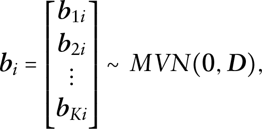
where
The multivariate GLMM provides a very flexible framework for modelling multiple longitudinal outcomes. Both frequentist and Bayesian estimation methods make use of the full joint likelihood derived from the joint distribution of the multiple longitudinal outcomes. In the frequentist paradigm, estimation is based on maximization of this joint likelihood. This is theoretically straightforward despite challenges in the case of non-Gaussian outcomes, where closed-form expressions are not obtainable and analytical approximations to the integrand or methods based on numerical integration are required (Wolfinger and O'Connell (1993); Breslow and Clayton (1993) and Gueorguieva (1999) for the multivariate case, Hedeker and Gibbons (1994, 1996); Pinheiro and Bates (1995, 2000); Fahrmeir and Tutz (1994)). In practice however, the dimensionality of the variance–covariance matrix for the random effects increases substantially as the number of outcomes increases, necessitating the simultaneous estimation of an unfeasibly large number of parameters. Moreover, numerical integration in high dimensions remains very challenging, even for those methods which perform better for higher dimensional data e.g., Monte Carlo methods, and specifically Monte Carlo EM and Monte Carlo Newton Raphson methods (McCulloch, 1997; Booth and Hobert, 1999).
An attractive alternative is Bayesian estimation, using MCMC methods to sample from the posterior distribution of the parameters (Gelfand and Smith, 1990; Robert and Casella, 2004; Gelman et al., 2013; Liu, 2001). For the multivariate GLMM, the posterior distribution is derived under the assumption of full conditional independence, that is, we assume that the longitudinal outcomes

where

Non-informative priors are typically used, specifically: independent univariate diffuse normal priors for the vector of fixed effects of each longitudinal submodel and an inverse-Gamma prior for the variance of the error terms, or alternatively, a half-Student's t prior with 3 degrees of freedom (when fitting a model with a normally distributed outcome). The covariance matrix of the random effects may be parametrized in terms of a correlation matrix
It is worth noting that in the Bayesian approach, the random effects are also considered model parameters for which we obtain a posterior sample. As a result, we are no longer required to solve the integral over the random effects. However, we are now required to (simultaneously) estimate an additional
Fieuws and Verbeke (2006) and Fieuws et al. (2007) propose a pairwise modelling approach as a potential solution to the computational problems encountered with the full multivariate model in the frequentist context. For

separately maximizing the log-likelihood of each pair
This technique is easy to fit with standard software, and the resulting estimates are consistent with the maximum likelihood estimates from the full multivariate model (Fieuws and Verbeke, 2006). Inference is somewhat more complicated however, and it should be noted that the estimates obtained are valid only for data that are missing completely at random (and specific cases of missing at random), since missing data might be dependent on specific outcomes not included in every pairwise model, or on combinations thereof.
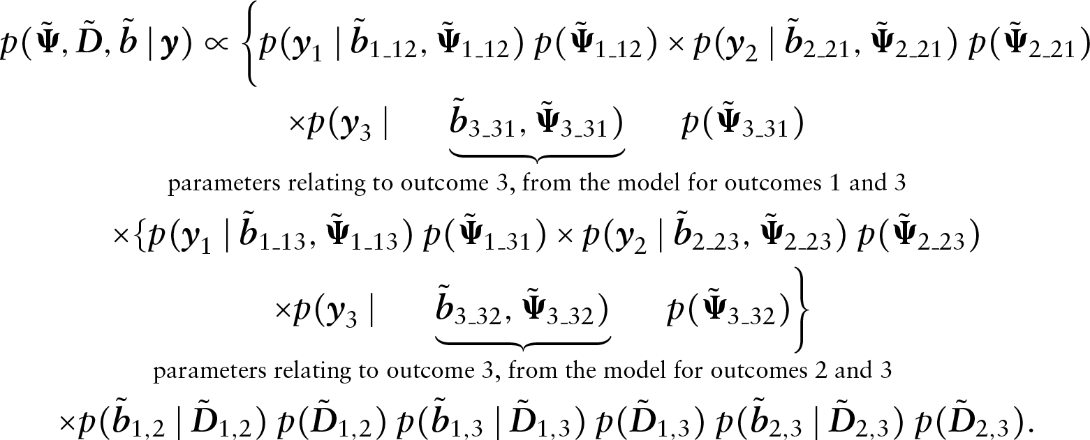
We propose an adaptation of the work by Fieuws and Verbeke (2006) to the Bayesian context, whereby we fit all of the
As is the case for Fieuws and Verbeke (2006), each outcome appears in
Let
We then obtain a combined sample

Note that throughout the article, the superscript
For example, where
In order to evaluate the performance of the pairwise approach, we performed a POC simulation study, comparing the finite sample properties of the pairwise and full multivariate approaches. In this setting, we simulated 300 subjects with a maximum of 9 repeated measurements per subject in 200 simulated datasets. We included

Eigenvalues, trace, and determinant of the posterior mean variance–covariance matrix for each approach in the POC simulation (Scenario A)

Eigenvalues, trace, and determinant of the posterior mean variance–covariance matrix for each approach in the POC simulation (Scenario A)
with
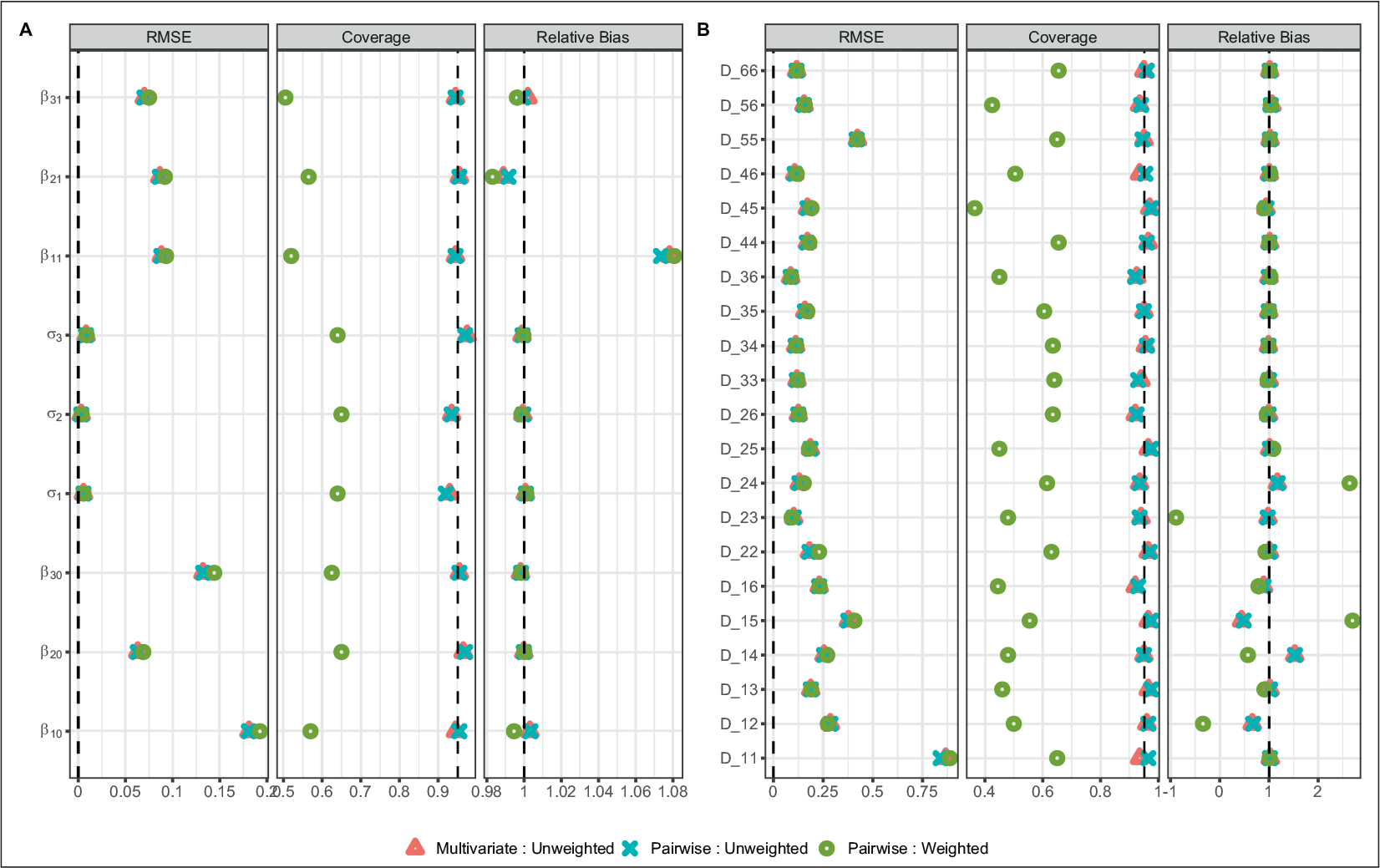
Per simulation, we obtained the sample marginal posterior distributions for each parameter using the multivariate and pairwise approaches, and calculated the posterior mean and 95% credible intervals. For each parameter, for each approach, we then assessed the relative bias (ratio) and coverage of the 95% credibile interval over all simulations, together with the root mean squared error (RMSE), and the relative efficiency, where the relative efficiency is defined as the ratio of the mean squared error of the multivariate and the pairwise approaches. The main concern lies with the reconstruction of the variance–covariance matrix for the random effects, since in the pairwise approach estimation proceeds independently for each constituent part of the full multivariate matrix. Figure 1 details the results for all parameters for the 200 simulated datasets. We see that the results from the two approaches are nearly identical, with minimal bias for the majority of parameters. Coverage was good, and there was no loss of efficiency. Based on these results, the performance of the pairwise approach is almost identical to that of the multivariate. We also obtain very similar eigenvalues, trace and determinant values for the variance–covariance matrix (Table 1).
The results thus far are not unexpected, given those obtained by Fieuws and Verbeke (2006). However, despite similarities seen in practice, the multivariate and pairwise approaches remain theoretically distinct. SNIS (MacKay, 2003; Owen, 2013) offers a potential solution. Importance sampling (IS) tells us that given a random variable 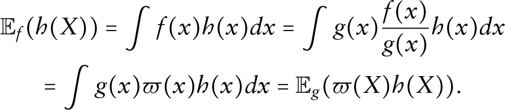
Relative bias, RMSE and coverage of the 95% credibile intervals for (A) fixed effect and residual variance parameters and (B) variance–covariance parameters in POC simulation scenario (Scenario A). Ideal values indicated by the vertical dashed lines are 0.95 for coverage, 1 for relative bias and 0 for RMSE. Variance–covariance parameters are represented by row and column position
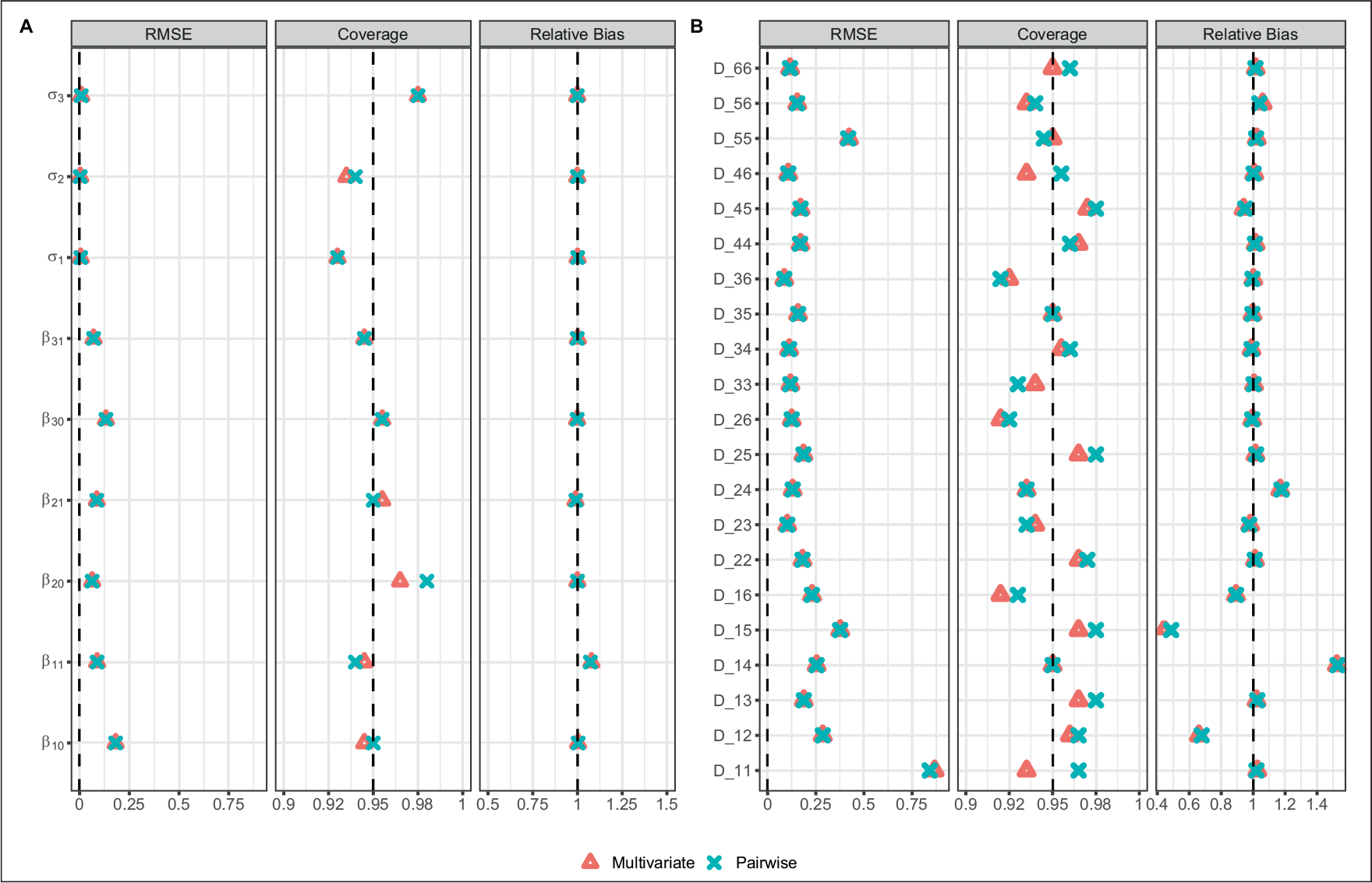
Relative bias, RMSE and coverage of the 95% credibile intervals for (A) fixed effect and residual variance parameters and (B) variance–covariance parameters in POC simulation scenario (Scenario A). Ideal values indicated by the vertical dashed lines are 0.95 for coverage, 1 for relative bias and 0 for RMSE. Variance–covariance parameters are represented by row and column position
Then the importance sampling estimate 
which implies that

We may only know 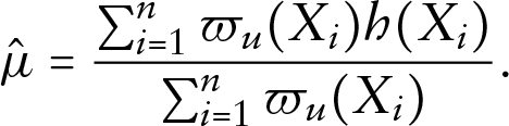
The 
where 
for
Recall that in the numerator, 
as the first set, necessitates the choice of

as the second set respectively. Defining 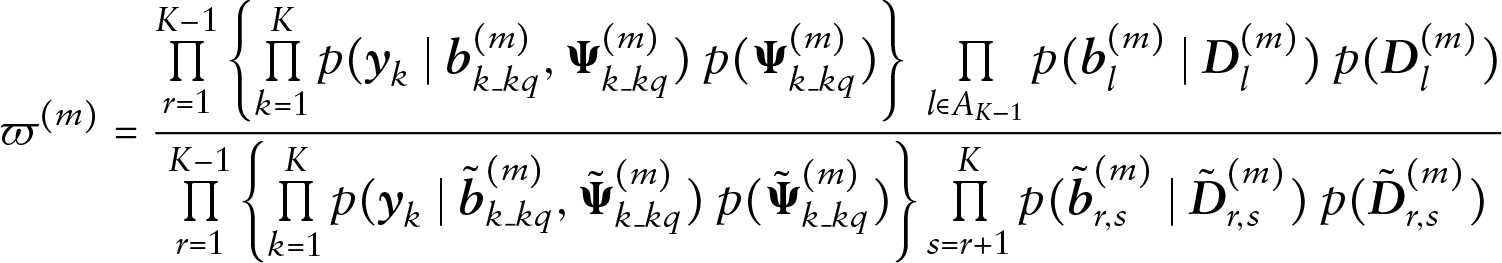
which simplifies to:
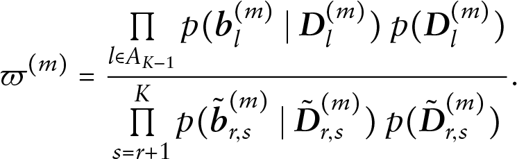
Where outcomes are related however, per iteration
We therefore investigate an alternative approach to obtain the variance–covariance matrix 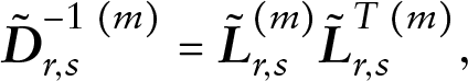
where 
for
As an informal check of the validity of (3.2), we evaluate it using the POC simulation setting, now specifying the outcomes as independent. In this setting, 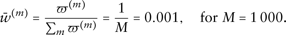
Using this approach for the three related outcomes in the POC simulation study, we are able to obtain a positive-definite matrix
Despite the reasonable performance of the matrix 
Relative bias, RMSE and coverage of the 95% credibile intervals for (A) fixed effect and residual variance parameters and (B) variance–covariance parameters in POC simulation scenario (Scenario A) with SNIS. Ideal values indicated by the vertical dashed lines are 0.95 for coverage, 1 for relative bias and 0 for RMSE. Variance–covariance parameters represented by row and column position
Relative bias, RMSE and coverage of the 95% credibile intervals for (A) fixed effect and residual variance parameters and (B) variance–covariance parameters in POC simulation scenario (Scenario A) with SNIS. Ideal values indicated by the vertical dashed lines are 0.95 for coverage, 1 for relative bias and 0 for RMSE. Variance–covariance parameters represented by row and column position
where
Given the instability of the weights, and the similarity of the results for the multivariate and unweighted pairwise approaches, we have elected to proceed with the unweighted pairwise approach. While the posterior distributions of the two approaches remain theoretically dissimilar, we believe that there is sufficient promise to the pairwise methodology to warrant further investigation of its performance.
We would expect this methodology to work well when the data is close to normal, since the normal distribution may be entirely described using only the first two moments. This is not necessarily true for other distributions however. We therefore performed two additional, more complex simulation studies, aimed at exploring how well the method copes with mixed outcomes (Scenario B), or settings in which there are no continuous outcomes, and a substantially reduced number of repeated measurements per subject (Scenario C). The results indicate that we are able to use the pairwise approach with minimal bias and loss of efficiency. Full details for both scenarios are available in Section A of the supplementary material.
Since we are able to run the pairwise models in parallel, there is a substantial decrease in the time taken to run the full multivariate model, and additionally, the pairwise approach enables us to obtain results for scenarios wherein the number of outcomes fully prohibits the use of the multivariate approach using standard software. The Bayesian adaptation of the pairwise approach also simplifies inference substantially.
The multivariate joint model for longitudinal and time-to-event outcomes
In the formulation of a multivariate joint model for multiple longitudinal outcomes and a time-to-event outcome, a GLMM is postulated as per (2.1) to accommodate the multivariate longitudinal outcomes. For the survival process, we denote by 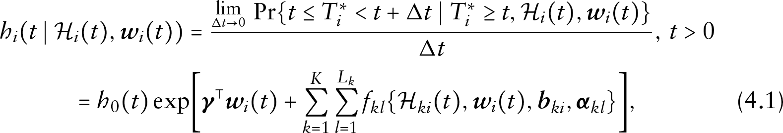
where
As noted in the introduction, Mauff et al. (2020) proposed an adaptation of a two-stage estimation procedure for a multivariate joint model for multiple longitudinal outcomes and a time-to-event outcome. They split the estimation procedure in two parts. In Stage I, they fit a multivariate GLMM for the longitudinal outcomes using either MCMC or HMC, and a sample of size M is obtained from the posterior:

where 
where 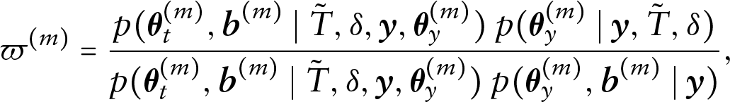
where the numerator is the posterior distribution of the multivariate joint model, and the denominator is the corresponding posterior distributions from each of the two stages. This becomes
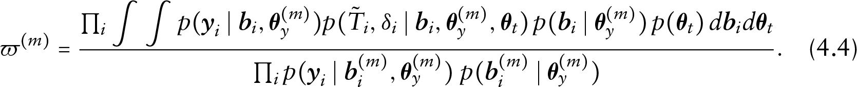
Further details may be found in the original article.
This method of estimation for the multivariate joint model is many orders of magnitude faster than the standard joint estimation. However, it remains bottlenecked by the necessity of fitting the full multivariate GLMM in the first stage. Despite the increase in speed, this method may therefore not accommodate situations where the number of longitudinal outcomes is very large. We are thus interested in whether or not the multivariate GLMM in Stage I may instead be estimated using the Bayesian pairwise approach outlined in this article.
The results obtained thus far using the pairwise approach are promising, even without the application of the SNIS correction. However, given that we are as yet unable to obtain a theoretically correct posterior distribution, we investigate its usefulness in the context of the joint model in a purely exploratory manner. We therefore do not adapt the entire corrected two-stage procedure for the joint model to incorporate the posterior distribution detailed in 3, and instead proceed as follows: per iteration
Simulation Scenarios D and E include 3 and 6 longitudinal outcomes, respectively, together with a survival outcome. For the survival outcome, adjusting for a binary group allocation, we used

where

for each outcome
Longitudinal evolution of continuous biomarkers (log base 2) for a randomly selected subset of individuals from the Bio-SHiFT cohort study that did/did not experience the primary event of interest

Longitudinal evolution of continuous biomarkers (log base 2) for a randomly selected subset of individuals from the Bio-SHiFT cohort study that did/did not experience the primary event of interest
In Mauff et al. (2020), the authors presented an analysis of the Bio-SHiFT study. The analysis focused on the association between the composite primary event of interest (consisting of hospitalization for heart failure, cardiac death, LVAD placement and heart transplantation) and each of six longitudinal biomarkers: Cystatin C (CysC), urinary N-acetyl-beta-D-glucosaminidase (NAG), kidney-injury-molecule (KIM)-1, N-terminal proBNP (NT-proBNP), cardiac troponin T (HsTNT) and C-reactive protein (CRP) (Figure 3).
As detailed in Mauff et al. (2020), for each of CysC, NAG and KIM-1 (
For the remaining outcomes (
where 
and included the baseline variables: age, sex, NYHA class (class III/IV vs. class I/II), use of diuretics, presence or absence of ischemic heart disease (IHD), diabetes mellitus, BMI and the estimated glomerular filtration rate (eGFR) value.
We compared the results obtained for this multivariate joint model using the corrected two-stage approach with the full multivariate GLMM, to those obtained using the pairwise approach as described, with and without the importance sampling weights for the joint model (once again updating the random effects in both cases). Full results are available in the supplementary material. As before, we are unable to obtain 95% credible intervals for the weighted results. We therefore limit our comparisons to the unweighted case: once again, we see very similar results regardless of which approach is used. However, as in simulation Scenario E, the variance–covariance parameters for the two approaches differ quite substantially. These parameters did not converge for the joint model when using the pairwise approach.
Discussion
In this article, we presented a Bayesian adaptation of the pairwise approach introduced by Fieuws and Verbeke (2006). We demonstrated that our approach works satisfactorily in the case of multiple longitudinal outcomes, with minimal bias, RMSE and good coverage even in scenarios where we have mixed or non-continuous outcomes. The Bayesian version is easy to implement, and inference is simpler than in the frequentist case. The use of this technique allows for faster computational times, since we are able to run the pairwise models in parallel. Moreover, it allows for the fitting of models in scenarios where the number of outcomes is so many as to entirely prohibit the use of the multivariate approach. We also explored the use of importance sampling weights in an attempt to obtain a theoretically proper multivariate posterior distribution. This was not successful: weights were obtained after several modifications but suffered from instability in the simulation settings presented here.
Incorporation of a time-to-event outcome was demonstrated using the corrected two-stage approach introduced in Mauff et al. (2020). The pairwise approach appears to work satisfactorily in the joint model context in only one of three analyses presented here. Comparing the unweighted results for the pairwise and multivariate approaches for simulation Scenario D, we found that they were very similar, with minimal bias, RMSE and good coverage of the 95% credible intervals for the majority of parameters, including the variance–covariance matrix of the random effects. However, the weights calculated for the joint model were once again unstable, which resulted in poor coverage. Interestingly, this occurred for both the multivariate and pairwise approaches. We anticipated potentially inferior results using the pairwise approach in the weighted case, since the formulation of these weights assumes a proper multivariate posterior distribution for the longitudinal submodel, which we do not have. However, the pairwise approach does not appear to have performed any worse than the multivariate. It is worth noting that the weights (while theoretically important) provide little in the way of meaningful practical change to the results for the corrected two-stage joint model, provided that the random effects are updated in the second stage.
In settings with a time-to-event outcome and a larger number of longitudinal outcomes however (simulation Scenario E and the analysis of the Bio-SHiFT data), comparing the unweighted results for the two approaches quite clearly demonstrates very large biases and RMSE for the variance–covariance parameters obtained using the pairwise approach. In these settings, the matrix
The large differences observed for these variance–covariance matrices may be due to issues in the construction of the matrix. Alternatively, the scale of the matrix prior to Cholesky decomposition may play a role. It could also be that the particular simulation settings chosen here were problematic: simulation of joint models with multiple longitudinal outcomes is challenging, especially the choice of values for the variance–covariance matrix. Interestingly, the remaining parameters of the longitudinal and survival submodels seem to be fairly robust to changes in the variance–covariance matrix, and consequently, the results for most of the remaining parameters from both the longitudinal and survival submodels were once again very similar for the two approaches.
A further issue of note is the instability of the importance sampling weights for both the multiple longitudinal outcomes case and the corrected two-stage joint model. The weights have previously been shown to work in the context of the joint model (Mauff et al., 2020). Additional exploration of the sensitivity of these weights is therefore warranted, as is further work on the incorporation of time-to-event outcomes when using the pairwise approach.
Footnotes
Supplementary materials
All relevant supplementary material and code referred to herein may be found through the link:
Acknowledgements
The first and last authors acknowledge support by the Netherlands Organization for Scientific Research VIDI grant nr. 016.146.301.
Declaration of conflicting interests
The authors declared no potential conflicts of interest with respect to the research, authorship and/or publication of this article.
Funding
The authors received no financial support for the research, authorship and/or publication of this article.