Random effect models for multivariate mixed data: A Parafac-based finite mixture approach

1 Introduction

Multivariate discrete and mixed responses have raised great interest in the recent past. In several empirical applications, from health econometrics, behavioural sciences, psychometrics among others, we may be interested in modelling individual choices as a function of observed covariates and a (possibly multidimensional) latent trait. To give some relevant examples, we may focus on measures of access to (and expenditures for) health care services to derive an indirect measure of individual health status; we may look at counts and types of purchases to describe individual consumer behaviours, or we may analyse responses to questionnaire items to get a deeper knowledge on personal traits. In all these cases, the univariate measures may be thought to depend on each other due to the presence of a (latent) common construct. Obviously, the measures can be observed on different scales: continuous for expenses, discrete for counts (of purchase or access), ordinal for items measuring self-perceived health status, categorical for types of purchase. Since a multivariate distribution with a proper and easily interpretable association structure is seldom available in such a context, a multivariate model can be defined by joining several conditional (univariate) models linked by a common latent construct. For this purpose, random effect models have received much attention in this context. Just to mention a few, the interested reader can give a look at the proposals by (Chib and Winkelmann (2001)), (Alfò and Trovato (2004)), (Rabe-Hesketh et al. (2005)), (Chipperfield and Steel (2012)), (Alfò and Rocchetti (2013)), (Jaffa et al. (2016)), (Oskrochi et al. (2016)) and (Husson et al. (2019)). Random effects provide a simple way to account for unobserved, individual-specific, heterogeneity, and to introduce a (simple) structure of dependence between outcomes. Parameter estimation is based on integrating these effects out of the complete data log-likelihood, usually adopting a parametric random effect distribution. (McCulloch et al. (2008)) give a comprehensive review of approaches to estimation in Generalized Linear Models with parametric random effects. Semi-parametric alternatives are also available. An unspecified, possibly continuous, random effect distribution can be in fact estimated by a discrete distribution, as noted, probably for the first time, by (Hinde and Wood (1987)). This approach is based on theoretical developments by (Laird (1978)) and (Lindsay(1983a); Lindsay(1983b) on the so called non-parametric maximum likelihood (NPML) estimation of a mixing distribution, see also (Simar (1976)) and (Böhning (1982)). The papers by (Aitkin (1996); Aitkin (1999)) have the important merit to complete the path: using discrete random effects we may describe heterogeneity/overdispersion in univariate and dependence in multivariate (longitudinal and clustered) outcomes, regardless the true shape of the random effect distribution. The corresponding approach could be labelled as semi-parametric, since we have a parametric specification for the conditional (regression) model and a non-parametric random effect (mixing) distribution. The corresponding observed data likelihood resembles that of a finite mixture of regression models, see (Quandt (1972)) and (Quandt and Ramsey (1978)) for early developments, and (Dietz (1992)) or (Wedel and DeSarbo (1995)) for extensions to GLMs. Maximum likelihood (ML) estimation is often carried out by using an EM-type algorithm. Among the several software implementations that have been proposed, we refer to the one available in the R library npmlreg, see (Einbeck et al. (2018)).

When we move to multivariate mixed data, however, the semi-parametric approach has a significant drawback when compared to its parametric counterpart, based on multivariate Gaussian random effects. With Gaussian assumptions, unobserved heterogeneity is described by profile-specific variances, while dependence between random effects in different outcome equations is described by the covariance terms. That is, independence (null off-diagonal entries in the covariance matrix) does not necessarily imply absence of heterogeneity (null diagonal entries). Indeed, as discussed by (Alfò and Rocchetti (2013)), the semi-parametric approach is based on a unidimensional, discrete, latent variable, with the same number of components in each marginal profile. In this case, multivariate dependence is based on heterogeneity, and both are present if and only if the number of components K is strictly greater than 1. Since the latent variable can be either unidimensional or multidimensional, depending on the nature of the problem and the impact it has on the manifest (observed) responses, we propose to extend the bivariate approach by (Alfò and Rocchetti (2013)) to the general multivariate one. We show how outcome-specific heterogeneity can be separated from dependence, so that the dependence model properly nests the independence one. The multivariate probability distribution for the random effects is now represented by a tensor with as many dimensions as the number of analysed outcomes, and model parameters can be straightforwardly estimated via ML. Since the dimension of the tensor grows with the number of outcomes, we may soon lose interpretability of the structure of dependence between the random effects. To solve this issue and make interpretation easier, we introduce a parsimonious parametrization of this tensor; this is based on a two-level hierarchy. Observed outcomes are independent conditional on (outcome-specific) random effects that are independent conditional on a (higher level) latent class. This parametrization of the joint probability tensor is based on the Parafac model introduced by (Harshman (1970)) and (Carroll and Chang (1970)). In its standard form, the Parafac is a generalization of factor analysis to tensors with more than two dimensions; the example is usually the so-called three-way data, where the same variables are collected on a sample of units at different occasions. In the present context, fitting the Parafac to the joint probability tensor offers a much simpler reading of the joint probability distribution in terms of a small number of latent classes that account for dependence between outcomes.

The article is structured as follows. In Section 2, we introduce a benchmark dataset which will be further analysed to discuss the aims and the features of the proposed model specification. In Section 3, we review the standard finite mixture approach to modelling multivariate responses. In Section 4, we propose a model that allows for more general dependence structures when p responses are observed. Section 5 describes how the Parafac model can be applied to reduce the number of free parameters in the proposed approach. The application to benchmark data is discussed in Section 6. Some concluding remarks are given in Section 7.

2 An illustrative example: NMES data

For illustration purposes, we discuss the re-analysis of data from a well-known survey; to be more specific, we propose a multivariate regression model for two measures of utilization of health care services, and a binary indicator for private insurance coverage. The motivation comes from the need to describe individual variability in the access to (and utilization of) health care services, as a function of individual characteristics, including the choice for a private insurance scheme.

Cost and appropriate access to health care services are fundamental issues for any modern health-care system, especially if we look at the elderly, a frail component of the population that is expected to increase in relative size. To analyse health needs and health services utilization by the elderly, (Deb and Trivedi (1997)), (Munkin and Trivedi (1999)) and (Deb et al. (2006)) considered data on individuals aged 66 and over (4 405 observations) from the National Medical Expenditure Survey (NMES), a study conducted in 1987–1988 to describe the use and payment for health services by US citizens. The NMES is based on a probability sample, representative of the whole US non-institutionalized population. In addition to health care data, the NMES provides information on (self-perceived) health status, employment, social, demographic and economic features. All individuals are covered by Medicare, a public insurance programme that guarantees protection against health care costs. Most individuals also make the choice for a supplementary private insurance scheme, shortly before their 65th birthday, as the price for such a scheme rises sharply with age and coverage is substantially lower. We re-analyse such data and consider two measures of health services utilization: the number of visits to an emergency room ( Emr ) and the number of hospital stays ( Hosp ).

Our aim is to explore the impact that individual features have on these measures of utilization, taking into account the structure of dependence with the aim at deriving information on common behavioural traits connected to health status. Available individual features include self-perceived health status, objective frailty status measured by chronic conditions and health-related problems that limit everyday life, demographic and socio-economic status, private insurance coverage ( Privins ). In Table 1, we report some exploratory statistics on the available sample.

OPEN IN VIEWER

Table 1

NMES data. Variable definitions and summary statistics. n = 4405

Variable	Definition	Mean	SD	Min	Max
Emr	Number of emergency rooms visits	0.26	0.70	0	12
Hosp	Number of hospitalizations	0.30	0.75	0	8
ExcHealth	1 if self-perceived health is excellent, 0 else	0.08
PoorHealth	1 if self-perceived health is poor, 0 else	0.13
NumChrCond	Number of chronic conditions	1.54	1.35	0	8
AdLim	1 if the personal condition limits daily life, 0 else	0.20
West	1 if the person lives in Western USA, 0 else	0.18
Age	Age in years (divided by 10)	7.44	0.63	6.6	10.9
AfroAmer	1 if African American, 0 else	0.12
Male	1 if male, 0 else	0.40
Married	1 if married, 0 else	0.55
EdYears	Number of years of education	10.3	3.74	0	18
Employed	1 if employed, 0 else	0.10
Privins	1 if covered by private health insurance, 0 else	0.78
Medicaid	1 if covered by Medicaid, 0 else	0.09

We must notice, however, that the effect of Privins on measures of utilization may not be that simple to interpret. In fact, two different mechanisms, with different implications from a health policy perspectives, may be at play. Individuals may select themselves into a private insurance coverage as a function of their preferences, socio-economic status, health status and expected future need for health care services. Therefore, the observed differences in utilization between those who have chosen a private insurance plan and those who have not may reflect, at least partially, this selection effect. As per the second mechanism, we may observe an increased utilization induced by lower (out-of-pocket) costs of care associated to private health insurance coverage, according to so-called moral hazard.

To analyse these sources of variation in utilization rates, as suggested by (Deb et al. (2006)), we need to model both the selection mechanism (i.e., the choice for private insurance conditional on individual characteristics) and the utilization counts conditional on the individual insurance status. Clearly, the (selection) process leading to the choice for private insurance is a function of both observed and unobserved factors, and the latter may also affect the utilization counts. For this reason, we need to define a multivariate model that accounts for dependence between the random effects in the equations for ( Emr , Hosp ) and Privins , respectively; that is, a regression model for the trivariate mixed response ( Emr , Hosp , Privins ). In the following sections, we briefly discuss the standard approach based on discrete random effects and, then, we introduce our proposal.

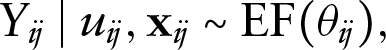
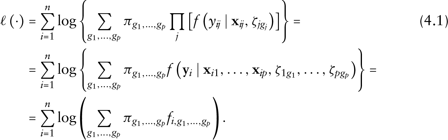
Let us assume that we have observed response values y ij on i = 1 , … , n , units for j = 1 , … , p , outcomes ( p = 3 in the application to the NMES data), together with outcome-specific covariates sets x ij , where x ij 1 = 1 , ∀ j = 1 , … , p . Since a proper multivariate model is not available for mixed type responses (here, two counts and a binary indicator), we model dependence between outcomes assuming they share some common, unobservable, features. In the case of health services utilization, these may refer to unobserved health status, individual propensity to use a specific health service, and so on. Let u ij , i = 1 , … , n , j = 1 , … , p , denote the unit- and outcome-specific random effects that account for heterogeneity in the univariate profiles and dependence between the profiles. We assume that the responses Y ij are independent conditional on the observed covariates and the random effects, with (conditional) density in the exponential family

Y ij ∣ u ij , x ij ∼ EF ( θ ij ) ,

with canonical parameter θ ij . To account for observed heterogeneity, we define a set of regression models for the conditional means:

Y ij ∣ x ij , u ij = ψ x ij ′ β j + u ij , i = 1 , … n , j = 1 , … , p ,

(3.1)

where ψ ( · ) represents the so called response function. Depending on the specific member of the exponential family, a regression model could be defined for mean and variance, as in the case of Beta regression, see, for example, Grün et al. (2012). Here, β j is an outcome-specific vector of regression parameters that are constant across units; the model specification is completed by assuming that the random effect vector u i = ( u i 1 , … , u ip ) has multivariate density g ( · ∣ Φ ) , where Φ denotes a set of parameters, and E ( u i ) = 0 , to ensure identifiability. Based on the conditional independence assumption, the likelihood function is:

L β , Φ = ∏ i = 1 n ∫ U ∏ j = 1 p f y ij ∣ x ij , u ij , β j g ( u i ∣ Φ ) d u i ,

(3.2)

where β = { β 1 , … , β p } . As it can be noticed, the likelihood in equation (3.2) refers to a two-level hierarchy, where outcomes are nested within units. We also need to consider potential correlation between u ij and x ij , see, for example, (Bates et al. (2014)) for a recent review on possible solutions. For Gaussian random effects, the marginal likelihood cannot be written in a closed form; to obtain ML estimates, we may use numerical integration techniques based on Gaussian quadrature, see (Rabe-Hesketh et al. (2005)), or on Monte Carlo/simulation techniques, see (Chib and Winkelmann (2001)) and (Munkin and Trivedi (1999)). Parametric approaches are often computationally intensive; for example, complexity of marginal maximization using Gaussian quadrature schemes grows exponentially with the number of outcomes.

A potential alternative approach is to provide a NPML estimate for g ( · ) , which can be proved to be a discrete distribution on K ≤ n support points, see (Laird (1978)), (Lindsay(1983a); Lindsay(1983b), (Simar (1976)) and (Böhning (1982)). We assume that this distribution puts masses π k on locations (support points) ζ k = ( ζ 1 k , … , ζ pk ) , where ζ jk represents the k th location for the j th profile, k = 1 , … , K , j = 1 , … , p . The resulting likelihood function is:

L β , ζ = ∏ i = 1 n ∑ k = 1 K π k ∏ j = 1 p f y ij ∣ x ij , ζ jk ,

(3.3)

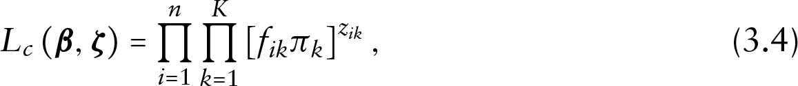
where ζ = { ζ 1 , … , ζ K } and π k = Pr ( u i = ζ k ) , k = 1 , … , K . Let us define the component indicator z i = ( z i 1 , … , z iK ) , i = 1 , … , n , with z ik = 1 if the i th unit comes from the k th component, characterized by u i = ζ k . We assume that the component indicator z i , i = 1 , … , n , has a multinomial distribution, with probabilities π k , k = 1 , … , K . The complete data likelihood is:

L c β , ζ = ∏ i = 1 n ∏ k = 1 K f ik π k z ik ,

(3.4)

where f ik = ∏ j = 1 p f ijk = ∏ j = 1 p f ( y ij ∣ x ij , ζ jk ) , i = 1 , … , n , k = 1 , … , K . Since the component indicators are unobserved, the EM algorithm arises quite naturally. In its basic form, the algorithm is run for a fixed number of components K which is chosen a posteriori using some external criteria. Usually, these are based on penalized likelihood, even if this is somewhat in contrast with the spirit of NPML estimation, see (Böhning (2000)). Following (Karlis and Meligkotsidou (2007)), we used AIC to choose the numbers of components as it provides, in our opinion, a more refined estimate of the mixing distribution when compared to BIC (Schwarz (1978)), CAIC (Bozdogan (1987)) or ICL (Biernacki et al. (2000)). Large-sample asymptotic normality for mixture models may fail to hold, and the result is, usually, that AIC tends to select too many components. This is usually not an issue in random intercept models, and it can be controlled by looking at the behaviour of model parameter estimates as K is increased.

At the t th step ( t = 1 , 2 , … ) of the algorithm, we calculate the expectation of the complete data log-likelihood ℓ c ( · ) conditional on the observed data y and the current ML parameter estimates Ψ ̂ ( t − 1 ) :

Q Ψ ∣ Ψ ̂ ( t − 1 ) = E Ψ ̂ ( t − 1 ) ℓ c ( · ) ∣ y = ∑ i = 1 n ∑ k = 1 K w ik ( t ) log ( f ik ) + ∑ i = 1 n ∑ k = 1 K w ik ( t ) log ( π k ) ,

(3.5)

where

w ik ( t ) = f ik ( t − 1 ) π k ( t − 1 ) ∑ l = 1 K f il ( t − 1 ) π l ( t − 1 ) .

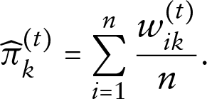
Taking derivatives of Q Ψ ∣ Ψ ̂ ( t − 1 ) , we obtain score equations that are weighted versions of standard score equations for homogeneous GLMs, with weights w ik , i = 1 , … , n , k = 1 , … , K , computed by using the joint p -dimensional distribution. For the prior probabilities, we obtain the usual (finite mixture) solution:

π ̂ k ( t ) = ∑ i = 1 n w ik ( t ) n .

Therefore, for units in the k th component of the finite mixture (with weight π k ) k = 1 , … , K , we have that the following model holds for the j th outcome, j = 1 , … , p :

Y ij ∣ x ij , z ik = 1 = ψ x ij ′ β j + ζ jk , i = 1 , … n , j = 1 , … , p .

(3.6)

In the following we will refer to this as the standard finite mixture approach.

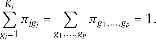
While the standard finite mixture approach is computationally efficient when compared to its parametric counterpart, it is based on the hypothesis that a unidimensional latent variable is enough to describe unobserved heterogeneity within outcomes and dependence between outcomes. This may lead to problems when several outcomes are considered and the task is to describe their association structure and/or to test for dependence. First, the univariate distributions cannot be derived by marginalizing the multivariate one; and they could be described by univariate random effect models with a possibly different number of components. Second, when considering mixed outcomes, we should bear in mind that the log-likelihood function is not a relative quantity; therefore, a different weight is associated to each outcome when building up the global log-likelihood; and the weight depends on the corresponding range of variation. That is, the number of components in the finite mixture model for multivariate outcomes may be driven only by a subset of the analysed outcomes. For all these reasons, following (Alfò and Rocchetti (2013)), we propose a different parametrization for the prior distribution: it allows a different number of components to be used for each outcome, and it leads to a multivariate model which properly nests the univariate ones. We denote by ζ jg j , π jg j , g j = 1 , … , K j , the locations and masses associated to the j th profile, j = 1 , … , p , where π jg j = Pr ( u ij = ζ jg j ) . When looking at the multivariate outcome, a joint mass π g 1 , … , g p = Pr ( u i 1 = ζ 1 g 1 , … , u ip = ζ pg p ) is associated to the p -tuple of locations, g j = 1 , … , K j , j = 1 , … , p . Under this model specification, marginals control for unobserved heterogeneity in the univariate profiles, while the joint probability distribution describes the association between the (locations in the) p profiles. This approach can be considered as a standard finite mixture model with K = ∏ j = 1 p K j components, where each component describes a specific p -tuple ζ 1 g 1 , … , ζ pg p . Clearly, when p = 1 , the proposed model reduces to a standard univariate finite mixture model. The following equation describes profile-specific (marginal) masses:

π jg j = ∑ g 1 , … , g j − 1 , g j + 1 , … , g p π g 1 , … , g p , j = 1 , … , p , g j = 1 , … , K j ,

under the constraint

∑ g j = 1 K j π jg j = ∑ g 1 , … , g p π g 1 , … , g p = 1 .

Thus, ∏ j K j − 1 free parameters have to be estimated, and, from a computational point of view, this approach is as complex as those based on Gaussian quadrature techniques. However, we should stress, at least, two differences. First, the number of locations is outcome-specific; that is, we may consider a low number of locations for profiles with low heterogeneity. Second, the locations and prior probabilities are not constrained to represent the discretization of a standard Gaussian distribution. Therefore, for a given level of heterogeneity, the number of locations may be lower than the number of Gaussian quadrature abscissas. The log-likelihood function is

ℓ · = ∑ i = 1 n log ∑ g 1 , … , g p π g 1 , … , g p ∏ j f y ij ∣ x ij , ζ jg j = = ∑ i = 1 n log ∑ g 1 , … , g p π g 1 , … , g p f y i ∣ x i 1 , … , x ip , ζ 1 g 1 , … , ζ pg p = = ∑ i = 1 n log ∑ g 1 , … , g p π g 1 , … , g p f i , g 1 , … , g p .

(4.1)

In this case, the standard EM algorithm for parameter estimation should be modified. Section 1 of the Supplementary Material describes its structure. The approach is simple to implement, and ML estimates simple to be derived (with issues typical of finite mixture models). We may, however, observe that the structure of dependence between outcomes, summarized by the joint probability distribution π g 1 , … , g p , g j = 1 , … , K j , j = 1 , … , p , can be quite difficult to interpret. If we denote by p the number of dimensions of the joint probability tensor Π _ , we may observe that, as p grows, visualizing and interpreting the dependence structure becomes more and more difficult. Thus, it is important to find a simplification that may help describe the dependence between outcomes in a simple, but still effective, way. This is exactly the purpose of our proposal.

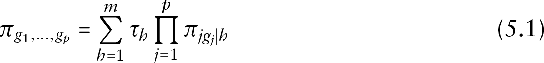
Let us consider π g 1 , … , g p , the generic element of the joint (multidimensional) probability tensor Π _ , g j = 1 , … , K j , j = 1 , … , p . According to (Dunson and Xing (2009)), such elements can be exactly decomposed as

π g 1 , … , g p = ∑ h = 1 m τ h ∏ j = 1 p π jg j ∣ h

(5.1)

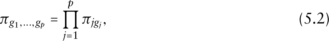
for an appropriate choice of m . This parametrization could be interpreted in terms of a latent class model, where h indexes a higher level discrete latent variable, see (Haberman (1979)); or we may consider it as a specific version, with non-negative terms, of the Parafac model, proposed by (Harshman (1970)) and (Carroll and Chang (1970)), see (Kroonenberg (2008)) for an overview. The value m can be associated with the rank of the tensor (Kruskal (1977)), and its role can be explained by noticing that, for m = 1 , we get

π g 1 , … , g p = ∏ j = 1 p π jg j ,

(5.2)

that is, we obtain the independence model. While the value of m controls for dependence between the random effects in the p outcome equations, m = 1 does not necessarily imply K j = 1 , ∀ j = 1 , … , p , or to be more explicit, outcome-specific unobserved heterogeneity and dependence between outcomes are kept separate. Just to give an example, for the NMES data this would mean that unobserved heterogeneity in the Emr equation may need a different number of components than that used in the equations for Hosp and Privins . Further, one or few components in the Emr profile may be associated with specific components in Hosp and Privins , and this may help characterize specific individual behaviours of interest. In this sense, the real merit of the Parafac representation is to make the joint random effect distribution more easy to interpret, by just looking at the values of m and π jg j ∣ h , j = 1 , … , p , g j = 1 , … , K j , h = 1 , … , m , associated to the different profile-specific components. These components may be interpreted by looking at the estimates for the corresponding intercepts.

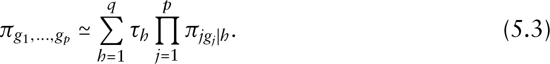
In a sense, the Parafac representation defines a regression model for the elements of the joint distribution π g 1 , … , g p , g j = 1 , … , K j , j = 1 , … , p . According to (Vermunt (2010)), it is often preferable not to estimate the parameters of such secondary models within the EM algorithm. Rather, so-called two- or three-step approaches should be used for this purpose; in a first step, model parameters are estimated using the EM algorithm; in a second step, units are proportionally allocated to components with weights given by posterior probabilities of component membership. In the third step, a multinomial logit is fitted to estimate the effects that observed covariates have on class membership. This is a good approach and, when the number of components is not large, it performs well in both real and simulated data. In the present context, the number of components is equal to ∏ j = 1 p K j and the resulting data matrix would be of order ( n × ∏ j = 1 p K j ) with several null entries (those associated to components that are unlikely for that unit). Therefore, we decided to take a different route, while retaining the idea of two-step approaches. First, we note that, differently from the rank of a matrix, the rank of a tensor can be higher than the dimensions of the tensor itself, that is we may have m > min ( K 1 , … , K p ) . The idea here is to approximate the joint distribution by using a limited number ( q ≤ m ) of latent components that are optimal in the least-squares sense:

π g 1 , … , g p ∑ h = 1 q τ h ∏ j = 1 p π jg j ∣ h .

(5.3)

By using the Parafac representation, for every profile j = 1 , … , p , and higher-level class h = 1 , … , q , ( K j − 1 ) elements π jg j ∣ h are free to vary in the interval [ 0 , 1 ] , whilst the latter one is constrained due to the unit-sum. The number of parameters is ( ∑ j = 1 p K j − p ) q ; using the same reasoning, ( q − 1 ) values τ h are free to vary. It follows that the total number of free parameters in the Parafac parametrization for Π _ is ( ∑ j = 1 p K j − p ) q + ( q − 1 ) , which can be much lower than the number of free elements of the tensor, ∏ j = 1 p K j − 1 .

This approach, referred to in the following as Parafac-based, is also motivated by the fact that, unlike the case of observed individual-level covariates, the models in equations (5.1) and (5.3) include only margin-specific intercepts. We propose to use the estimates of π g 1 , … , g p , g j = 1 , … , K j , j = 1 , … , p , obtained within the EM algorithm, to fit the Parafac model with q (higher-level) classes, and obtain a more parsimonious and easy to interpret parametrization. This process, where the Parafac step is embedded within the EM algorithm, is repeated until convergence. The technical details of the additional steps in the EM algorithm that we use to estimate the parameters in the Parafac parameterization are described in Section 2 of the Supplementary Material. Here, we briefly sketch the structure of the algorithm for fixed q and K j , j = 1 , … , p .

Step 0 Set ε > 0 (e.g., ε = 10 − 6 ), at step t = 1 , 2 , …

Taking inspiration from (Vermunt (2010)), an alternative, two-step, sequential strategy can also be considered: the EM algorithm is run first, and Steps 4–7 are performed, at convergence, outside the EM algorithm, by fitting the model in equation (5.3) to final estimates π ̂ g 1 , … , g p . The sequential strategy is a computationally efficient approximation to the embedded one; our preliminary findings suggest that the two strategies usually lead to very similar solutions. For this reason, we suggest to use the embedded strategy for estimating model parameters and the sequential one for deriving confidence intervals (CIs) based on non-parametric bootstrap.

Obviously, if we do not use the Parafac parameterization, Steps 4–7 are simply skipped, and we obtain the algorithm for the general solution, characterized by the choice q = m .

As a starting point, we fitted univariate regression models for Emr and Hosp ; these are based on (conditional) Poisson distribution, log link function and discrete, individual-specific, random effects. We used the npmlreg library (Einbeck et al. (2018)) to obtain estimates, and selected, using AIC, ( K 1 , K 2 ) = ( 2 , 3 ) components (locations) for Emr and Hosp , respectively. As expected, private insurance coverage is (barely) significant only in the equation for Hosp . Parameter estimates are reported in Section 3 of the Supplementary Material.

As a second step, we considered a further model for the private insurance choice. This is based on a (conditional) Bernoulli distribution, logit link function, and discrete individual-specific random effects. Also in this case, we used the npmlreg library, and selected K = 2 components by using AIC. By joining these model estimates with those for Emr and Hosp reported in Section 3 of the Supplementary Material, we observe that the optimal choice of the number of components, according to AIC, is ( K 1 , K 2 , K 3 ) = ( 2 , 3 , 2 ) for the three outcomes, Emr , Hosp and Privins , respectively.

We used such a choice to fit the proposed multivariate model, where we set q = 2 looking for simplicity and checking for accuracy of the resulting approximation. We may also notice that such a choice is optimal (according to AIC) conditional on setting ( K 1 , K 2 , K 3 ) = ( 2 , 3 , 2 ) . Clearly, a different choice could be obtained by simultaneously searching for the best ( K 1 , K 2 , K 3 , q ) values; we have preferred the proposed procedure to have a direct comparison with the results obtained by fitting univariate models for each outcome. A further motivation is that the number of components in each margin is essentially due to unobserved heterogeneity and, therefore, we cannot see any reason to change it when moving from the univariate to the multivariate model. The joint distribution accounts for dependence between outcomes and, in this view, the number of classes q is of interest, as it controls for dependence and quality of approximation to the true Π _ .

We have also used different sets of observed covariates for the three outcome equations, considering for the utilization counts only those directly referring to perceived, objective health status and ageing, and leaving for the private insurance equation all individual-specific socio-economic and demographic features. This has been done to have an efficient model structure, according to a specific graph of dependence and, therefore, to a specific set of excluding restrictions, see (Kiviet (2020)) for an interesting discussion on this and related issues in model identification.

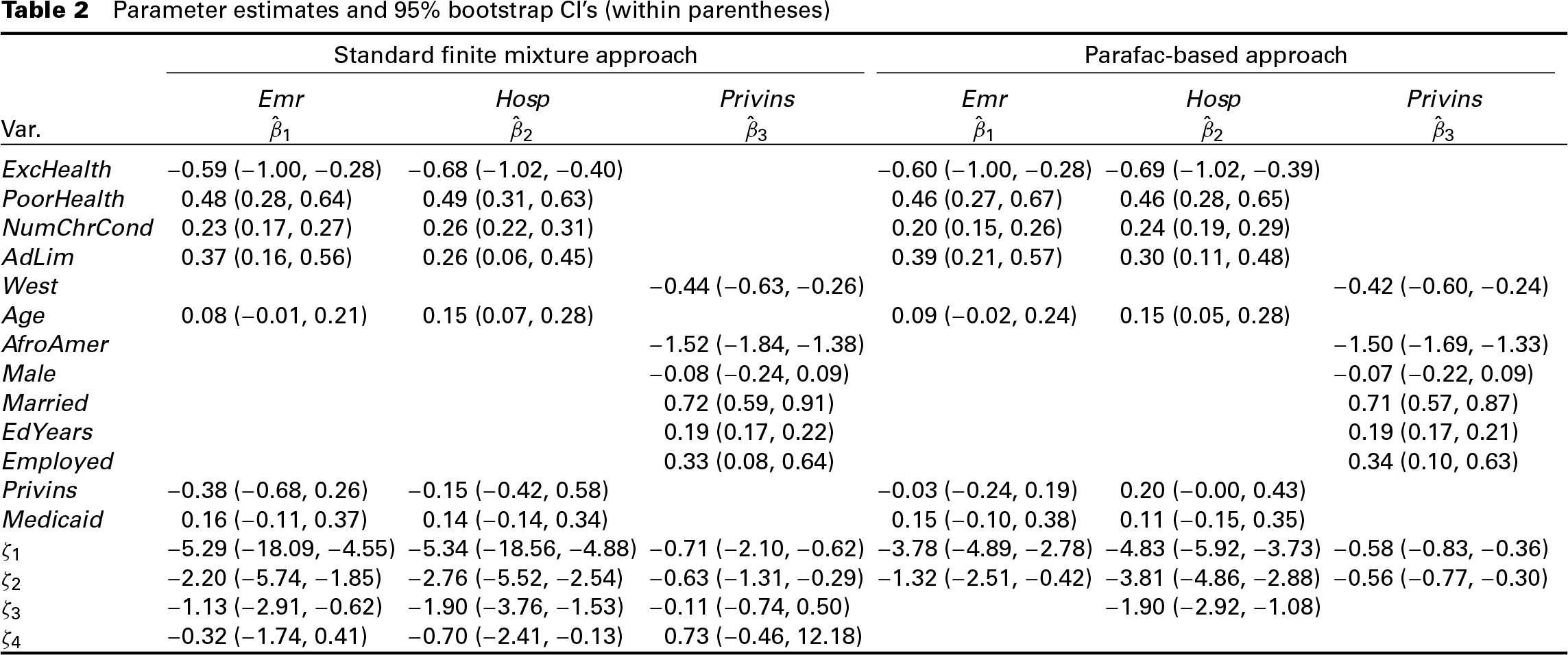
The results can be easily compared with those derived from the univariate regression models, as heterogeneity and dependence are now kept separated. We also fitted a standard finite mixture model, which is built by assuming that the estimated locations in the three equations are trivariate realizations of a single (unidimensional) random effect. In this case, the number of components in each profile, set according to AIC, is constant, that is, K 1 = K 2 = K 3 = K = 4 , and the dependence cannot be kept separated from unobserved heterogeneity. In Table 2, we report the estimates for the trivariate regression model, obtained by considering the standard finite mixture, and the proposed approach via the embedded strategy. The CIs have been obtained by non-parametric bootstrap using B = 1 000 resamples and the sequential strategy, where components are ordered by the location estimates (as in Table 2) for handling potential label switching.

OPEN IN VIEWER

Table 2

Parameter estimates and 95% bootstrap CI's (within parentheses)

	Standard finite mixture approach			Parafac-based approach
	Emr	Hosp	Privins	Emr	Hosp	Privins
Var.	β ̂ 1	β ̂ 2	β ̂ 3	β ̂ 1	β ̂ 2	β ̂ 3
ExcHealth	− 0.59 ( − 1.00, − 0.28)	− 0.68 ( − 1.02, − 0.40)		− 0.60 ( − 1.00, − 0.28)	− 0.69 ( − 1.02, − 0.39)
PoorHealth	0.48 (0.28, 0.64)	0.49 (0.31, 0.63)		0.46 (0.27, 0.67)	0.46 (0.28, 0.65)
NumChrCond	0.23 (0.17, 0.27)	0.26 (0.22, 0.31)		0.20 (0.15, 0.26)	0.24 (0.19, 0.29)
AdLim	0.37 (0.16, 0.56)	0.26 (0.06, 0.45)		0.39 (0.21, 0.57)	0.30 (0.11, 0.48)
West			− 0.44 ( − 0.63, − 0.26)			− 0.42 ( − 0.60, − 0.24)
Age	0.08 ( − 0.01, 0.21)	0.15 (0.07, 0.28)		0.09 ( − 0.02, 0.24)	0.15 (0.05, 0.28)
AfroAmer			− 1.52 ( − 1.84, − 1.38)			− 1.50 ( − 1.69, − 1.33)
Male			− 0.08 ( − 0.24, 0.09)			− 0.07 ( − 0.22, 0.09)
Married			0.72 (0.59, 0.91)			0.71 (0.57, 0.87)
EdYears			0.19 (0.17, 0.22)			0.19 (0.17, 0.21)
Employed			0.33 (0.08, 0.64)			0.34 (0.10, 0.63)
Privins	− 0.38 ( − 0.68, 0.26)	− 0.15 ( − 0.42, 0.58)		− 0.03 ( − 0.24, 0.19)	0.20 ( − 0.00, 0.43)
Medicaid	0.16 ( − 0.11, 0.37)	0.14 ( − 0.14, 0.34)		0.15 ( − 0.10, 0.38)	0.11 ( − 0.15, 0.35)
ζ 1	− 5.29 ( − 18.09, − 4.55)	− 5.34 ( − 18.56, − 4.88)	− 0.71 ( − 2.10, − 0.62)	− 3.78 ( − 4.89, − 2.78)	− 4.83 ( − 5.92, − 3.73)	− 0.58 ( − 0.83, − 0.36)
ζ 2	− 2.20 ( − 5.74, − 1.85)	− 2.76 ( − 5.52, − 2.54)	− 0.63 ( − 1.31, − 0.29)	− 1.32 ( − 2.51, − 0.42)	− 3.81 ( − 4.86, − 2.88)	− 0.56 ( − 0.77, − 0.30)
ζ 3	− 1.13 ( − 2.91, − 0.62)	− 1.90 ( − 3.76, − 1.53)	− 0.11 ( − 0.74, 0.50)		− 1.90 ( − 2.92, − 1.08)
ζ 4	− 0.32 ( − 1.74, 0.41)	− 0.70 ( − 2.41, − 0.13)	0.73 ( − 0.46, 12.18)

Looking at Table 2, we can derive some general implications of the proposed modelling approach. First, the estimates for the regression parameters in the standard finite mixture and in the proposed approach are quite similar. This is not unexpected, as the two parameterizations differ only in the specification of the random effect distribution: both the regression models consider only individual-specific random intercepts which, due to the cross-sectional nature of the available data, are considered to be (at least linearly) independent of the observed covariates. When we move from the standard finite mixture to the proposed approach, the structure of the random effects (joint) distribution changes. Therefore, as a second general implication of the proposed approach, we expect some changes in the variance-covariance (correlation) estimates for the random effect distribution, as well as in the point and interval estimates for the endogenous covariate, if any (in this case Privins ).

As per results specific to the analysed data, the estimates for the covariance/correlation matrix of the random effects are reported in Table 3. The variance estimates for the three random effects are quite different depending on whether we look at the standard or the proposed approach: while we cannot comment on which one is producing the best estimates (true values are unknown), we notice that the proposed approach produces random effect variance estimates in the equations for ( Emr , Hosp ) that are very similar to those obtained by fitting the univariate regression models. Further, while both approaches produce a low variance estimate for the random effects in the Privins equation, what substantially changes is the estimate for the correlation between the random effects in the Privins and those in the ( Emr , Hosp ) equations. As we can see from the right-hand side of Table 3, the estimates obtained by the standard finite mixture approach are surprisingly high. On the contrary, we get nearly null estimates for these terms by the proposed approach; according to this last result, the choice for the private insurance in this sample can be considered as exogenous. As stated in Deb and Trivedi (1997), this result is coherent with the empirical evidence that ‘(...) private insurance typically covers physical therapy, check-ups, etc., with small deductibles and coinsurance rates’. We also observe some changes in the estimates of the effect of the binary treatment variable Privins . The associated regression coefficients in the equations for ( Emr , Hosp ) stay, however, non-significant regardless of the structure we adopt for the joint distribution. In the standard finite mixture approach, the estimated locations for the Privins equation are strongly connected to those of the utilization counts, and this may induce some (unnecessary) higher variability in the parameter estimate for Privins in the utilization count equations, due to some overlapping between the private insurance indicator and a specific component. The confidence intervals for Privins in both utilization equations in the standard finite mixture approach are substantially wider than the one obtained with the proposed approach. This result is specific to the analysed example and it is probably due to the binary measurement scale of this response.

OPEN IN VIEWER

Table 3

Estimates of the covariance matrix of the random effects in the three regression models. Standard finite mixture and Parafac-based approach

	Covariance matrix						Correlation matrix
	Standard finite			Parafac-based			Standard finite			Parafac-based
	mixture approach			approach			mixture approach			approach
Var.	Emr	Hosp	Privins	Emr	Hosp	Privins	Emr	Hosp	Privins	Emr	Hosp	Privins
Emr	5.25	4.43	0.58	1.05	1.03	− 0.00002	1	0.99	0.76	1	0.91	− 0.002
Hosp		3.75	0.51		1.23	− 0.00002		1	0. 73		1	− 0.002
Privins			0.13			0.00013			1			1

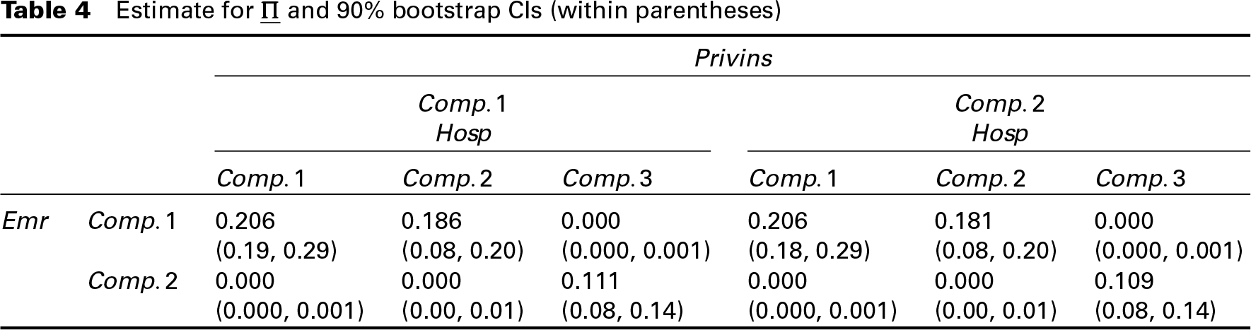
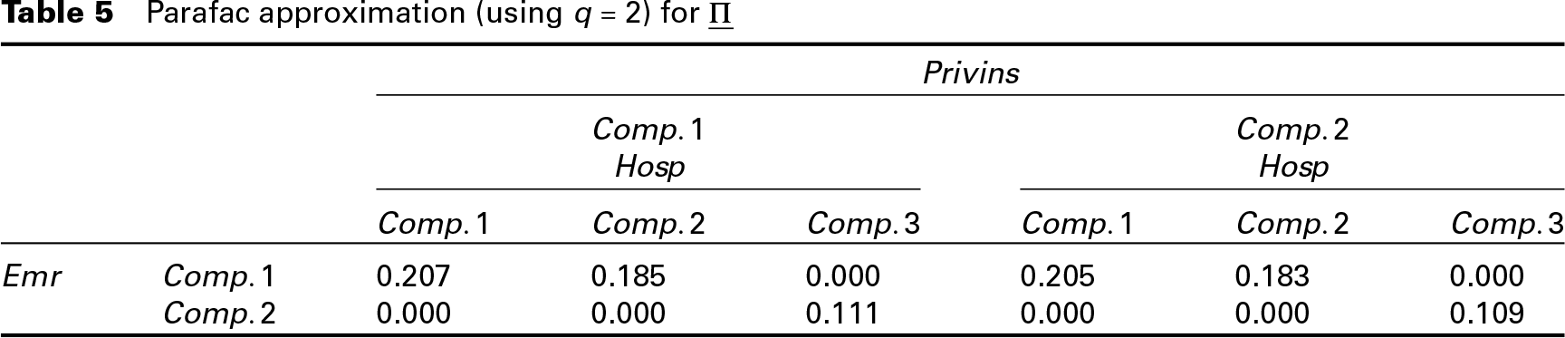
We now turn to discuss results associated to the proposed parameterization of the joint distribution for the specific application. As far as the choice for q is entailed, Table 4 reports the estimates of the elements of the joint probability tensor Π _ we obtain by the EM algorithm, without any specific parameterization. This is the best approximation possible to Π _ we may obtain by using a Parafac representation, as it is obtained without any dimensionality reduction. Therefore, we may consider it as obtained by the choice q = m (in this case, m = 3 ). We report in Table 5 the estimate obtained by setting q = 2 . We used a 1 − α = 0.9 confidence level to avoid issues related to poor mixing (that is nearly equal mass estimates) we observed (even if rarely) in the bootstrap solutions.

OPEN IN VIEWER

Table 4

Estimate for Π _ and 90% bootstrap CIs (within parentheses)

		Privins
		Comp . 1			Comp . 2
		Hosp			Hosp
		Comp . 1	Comp . 2	Comp . 3	Comp . 1	Comp . 2	Comp . 3
Emr	Comp . 1	0.206	0.186	0.000	0.206	0.181	0.000
		(0.19, 0.29)	(0.08, 0.20)	(0.000, 0.001)	(0.18, 0.29)	(0.08, 0.20)	(0.000, 0.001)
	Comp . 2	0.000	0.000	0.111	0.000	0.000	0.109
		(0.000, 0.001)	(0.00, 0.01)	(0.08, 0.14)	(0.000, 0.001)	(0.00, 0.01)	(0.08, 0.14)

OPEN IN VIEWER

Table 5

Parafac approximation (using q = 2 ) for Π _

		Privins
		Comp . 1			Comp . 2
		Hosp			Hosp
		Comp . 1	Comp . 2	Comp . 3	Comp . 1	Comp . 2	Comp . 3
Emr	Comp . 1	0.207	0.185	0.000	0.205	0.183	0.000
	Comp . 2	0.000	0.000	0.111	0.000	0.000	0.109

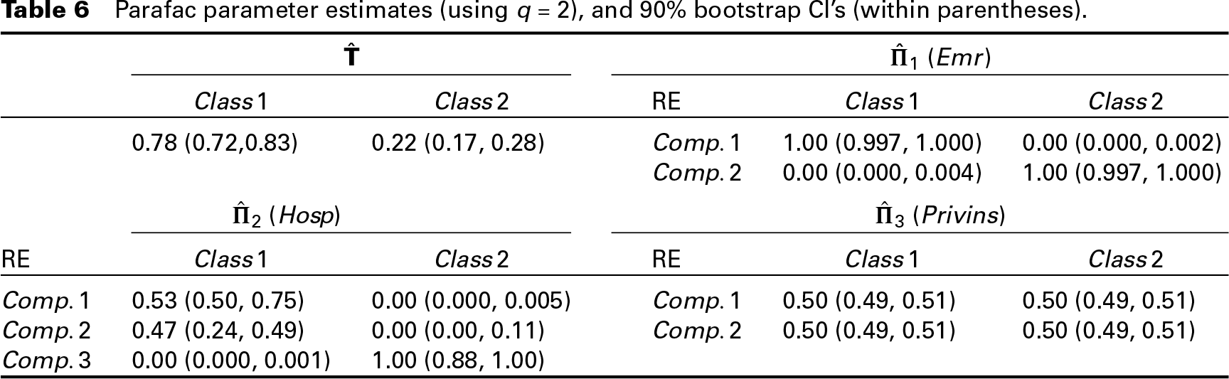
For purpose of estimation, we used the embedded strategy and a maximum of 50 iterations. Our preliminary analyses show that increasing this value implies a noticeable increase in the computational complexity without any substantial gain in terms of fitting. As noticed above, to save computation time, the algorithm for fitting the Parafac to Π _ (Steps 4–7) can be run once convergence is attained. Such a two-step strategy leads to virtually the same values for the log-likelihood function. As it is easy to observe, the estimates for q = m and q = 2 are virtually identical, and this suggests that the choice q = 2 is a good one. The quality of approximation dramatically decreases when moving to q = 1 , see Section 4 of the Supplementary Material. The estimate of Π _ in Table 5 is obtained by using the Parafac parameterization which, especially in those cases where the number of outcomes p is high, is much simpler to interpret, as it inherently refers to univariate components, see estimates in Table 6.

OPEN IN VIEWER

Table 6

Parafac parameter estimates (using q = 2 ), and 90% bootstrap CI's (within parentheses).

	T ̂			Π ̂ 1 ( Emr )
	Class 1	Class 2		RE	Class 1	Class 2
	0.78 (0.72,0.83)	0.22 (0.17, 0.28)		Comp . 1	1.00 (0.997, 1.000)	0.00 (0.000, 0.002)
				Comp . 2	0.00 (0.000, 0.004)	1.00 (0.997, 1.000)
Π ̂ 2 ( Hosp )				Π ̂ 3 ( Privins )
RE	Class 1	Class 2		RE	Class 1	Class 2
Comp . 1	0.53 (0.50, 0.75)	0.00 (0.000, 0.005)		Comp . 1	0.50 (0.49, 0.51)	0.50 (0.49, 0.51)
Comp . 2	0.47 (0.24, 0.49)	0.00 (0.00, 0.11)		Comp . 2	0.50 (0.49, 0.51)	0.50 (0.49, 0.51)
Comp . 3	0.00 (0.000, 0.001)	1.00 (0.88, 1.00)

A further argument is the characterization of the estimated latent structure. In the following, to make the discussion of results simpler, we will refer to categories h = 1 , 2 , of the higher level latent variable as classes, and to categories g j = 1 , … , K j , j = 1 , … , p , of the lower level latent variables (random effects) as components. Figure 1 reports the observed (marginal) distribution of ( Emr , Hosp ) by estimated components, where individual membership has been obtained by using a (profile-specific) maximum a posteriori (MAP) rule.

OPEN IN VIEWER Figure 1

Boxplots of Emr and Hosp by components. Allocation of individuals is based on a (profile-specific) MAP rule

From the left-hand side in Figure 1, we can see that the two components identify units with, respectively, a lower and a higher propensity to access an EMR conditional on observed individual characteristics, where the observed distribution for component 2 is noticeably more dispersed than that for component 1. From the right-hand side in Figure 1, we observe an increasing number of hospital stays, conditional on other observed individual characteristics, when moving from the first to the third component. Hence, estimated locations and associated components distinguish units with extreme, higher, values of Emr or Hosp from the bulk of units with small values, always conditional on observed covariates. However, these results do not account for the structure of dependence between the random effects in the two equations, which can be explained by looking at the higher level classes. The probability of latent class 1 is much higher than that of latent class 2; what does this mean from a practical perspective? To answer, we need to look at the distribution we estimate conditional on these latent classes. With respect to Emr , the first component (with an intercept estimate ζ ̂ 11 = − 3.78 ) is associated only with latent class 1, while the second component (with an intercept estimate ζ ̂ 12 = − 1.32 ) refers only to latent class 2. Therefore, if we look at these estimates, we may characterize class 2 as being composed of individuals that have, conditional on observed covariates, a higher propensity to access an emergency room. A similar behaviour is derived by looking at the components for Hosp , where the third component (with an estimate ζ ̂ 23 = − 1.90 ) is associated with latent class 2 only, while the other two, with lower estimates for the component-specific intercepts ( ζ ̂ 21 = − 4.83 and ζ ̂ 22 = − 3.81 ) are associated with latent class 1 only. Therefore, when we look at utilization measures, we may characterize latent class 1 as composed of people with a lower (conditional on individual covariates) utilization of the analysed health services, while latent class 2 is characterized by a higher propensity to use such services.

When we move to the parameter estimates for Privins , we may observe that the two latent classes essentially overlap, as the outcome-specific components are equally split into the two classes. As discussed before, from a modelling point of view, this may suggest that exogeneity of the private insurance choice cannot be ruled out.

Thus, the approximated solution obtained by the Parafac representation of the joint probability distribution helps to obtain a simpler description of the components associated to univariate outcome-specific random effects, while providing a more refined picture of the association between the random effects in the different equations and, through this, between the different outcomes.

In this article, we propose a flexible regression model for multivariate mixed responses. The model structure is based on considering several (conditionally independent) univariate regression models with outcome-specific random effects, that account for outcome-specific unobserved heterogeneity and dependence between outcomes through their joint distribution. The proposed representation of this joint distribution relaxes the unidimensionality assumption which is standard in (multivariate) finite mixture models, and it opens to more general structures of dependence between the random effects in the different outcome equations. While it is more general than standard finite mixture models, it is also more computationally demanding, as the complexity grows exponentially with the number of analysed outcomes. To tune the complexity of such a representation, we propose to use a parametrization which can be linked either to a polytomous latent class model or to a Parafac model for the tensor describing the joint probability distribution. The proposed representation is simple to estimate, by using an extended EM algorithm, and it gives an appropriate picture of unobserved heterogeneity and dependence. In particular, we may guess that the proposed approach gives more accurate estimates of outcome-specific random effect variances, as well as of covariances between the random effects in different outcome equations. This may be useful when the interest is on testing for dependence, especially in those cases where p ≫ 3 , which will be the focus for future research, especially from the perspective of computational complexity. The representation of the joint probability tensor Π _ we propose in this article can also be used within a stochastic EM, see, e.g., McLachlan and Krishnam (1997), algorithm, where component membership can be drawn from the Π _ estimate, and a polytomous latent class model is estimated on the basis of the simulated component labels.

The proposed model has been applied to benchmark real life data, which helped us to discuss, from an empirical perspective, the implications of the proposed approach.

Supplementary materials

The supplementary materials, which also include the relevant R code and the NMES data, can be found through the link: http://www.statmod.org/smij/archive.html