



Abstract
Common random effects models for repeated measurements account for the heterogeneity in the population by including subject-specific intercepts or variable effects. They do not account for the heterogeneity in answering tendencies. For ordinal responses in particular, the tendency to choose extreme or middle responses can vary in the population. Extended models are proposed that account for this type of heterogeneity. Location effects as well as the tendency to extreme or middle responses are modelled as functions of explanatory variables. It is demonstrated that ignoring response styles may affect the accuracy of parameter estimates. An example demonstrates the applicability of the method.
Keywords
Introduction
Random effects models are a common tool for the modelling of heterogeneity and dependence of responses in repeated measurements and clustered data. Binary and ordinal random effects models account for heterogeneity by including subject-or cluster-specific effects in the linear predictor. The most widely used model is the random intercept model which allows the overall tendency to positive responses to vary over subjects. In more general models also slopes can depend on the subject. However, there is one subject-specific trait that is usually ignored, the tendency to select extreme or middle categories. This tendency can be considered as a response style, which is a consistent pattern of responses that is independent of the content of a response (Johnson, 2003). The problem with response styles is that they can affect the validity of parameter estimates because estimates may be biased if the response style is ignored. Therefore, models should account for the response style to avoid misleading estimates. Response styles have been investigated in particular in the survey literature, but the phenomenon occurs whenever subjects give ratings on an ordinal scale. Further examples could be if a medical diagnosis refers to categories such as normal, borderline and abnormal or when patients rate their pain on a five-point scale. The phenomenon is found in all assessed ordinal categorical variables, which arise when an assessor processes an unknown amount of information, leading to the judgement of the grade of the ordered categorical scale (Anderson, 1984).
Response styles have been investigated in particular in the social sciences, see, for example, Messick (1991), Baumgartner and Steenkamp (2001), Marin et al. (1992) and Meisenberg and Williams (2008), and in latent trait modelling in psychometrics, see Bolt and Newton (2011), Johnson (2003), Eid and Rauber (2000), Böckenholt (2017) and Tutz et al. (2018). An overview was given by Van Vaerenbergh and Thomas (2013).
Binary and ordinal random effects models without the modelling of response style are well established tools. In particular, the case of binary response variables has been investigated thoroughly, see, for example, Hedeker and Gibbons (1994), Hinde (1982), Anderson and Aitkin (1985), Liu and Pierce (1994), Pinheiro and Bates (1995) and Booth and Hobert (1999). Also for ordinal responses, several modelling strategies and estimation methods have been proposed. Harville and Mee (1984), Jansen (1990) and Tutz and Hennevogl (1996) considered cumulative type random effects models; adjacent categories type models were considered by Hartzel et al. (2001).
Models that explicitly account for response styles are able to reduce the bias. They account for additional heterogeneity in the population, which in some applications is itself of interest, in particular if it is linked to explanatory variables. In this article it is argued that simultaneous modelling of response styles is recommended if response styles are present, more concisely, if individuals have a tendency to prefer middle or extreme categories. According to the classification of different types of response style by Van Vaerenbergh and Thomas (2013), these tendencies refer to a continuum between the so-called mid-point response style (MRS) and extreme response style (ERS). If response styles that vary over individuals are present but ignored, the accuracy of parameter estimates may suffer. Moreover, the models, that are proposed allow researchers to investigate which variables determine the preference for middle or extreme categories. It should be noted that methods that account for response tendencies have been used before in regression for univariate ordinal responses, see Tutz and Berger (2016, 2017). However, in univariate ordinal models, response styles are not modelled as a subject-specific trait but as a tendency that is determined by covariates only. Consequently, estimation methods that are used for univariate ordinal responses are quite different from the methods used here, where response style is meant to represent a consistent pattern of responses independent of the content. In a multivariate setting, response styles were incorporated by Tutz et al. (2018) within the partial credit model. However, their model lacks the possibility to include covariates.
The article is structured as follows. In Section 2, we introduce multivariate ordinal response models. In Section 3, we develop an approach to include response styles into multivariate ordinal response models, while in Section 4, we give further details of the estimation procedure. Section 5, illustrates the performance of the proposed method using a simulation study. Finally, in Section 6, the method is applied to data from the German Longitudinal Election Study (GLES).
Models for multivariate ordinal responses
Regression models for a single ordinal response form the constituents of multivariate models. Therefore, we first briefly consider models that are in common use for ordinal responses and then consider extensions to multivariate responses.
Ordinal response models
Interesting models for ordinal responses are in particular the cumulative model and the adjacent-categories model. With the response

where
Among the class of cumulative models, the most widely used model is the proportional odds model which uses the logistic distribution

With

that is,
An alternative model is the adjacent-categories model, which has the form

where

With

which is the change in local odds if
Also the so-called sequential model is used in ordinal regression but is less used in multivariate settings. For an overview on ordinal regression see Agresti (2009), Tutz (2012) and Peyhardi et al. (2015).
All of these models can be given in matrix form as multivariate generalized linear models (GLMs) for categorical responses. For observation

where

where
Random effects models
Random effects models aim at explicitly modelling the heterogeneity of clustered responses. A cluster can be any statistical unit for which repeated measurements are available. In our applications, a cluster typically refers to a person and repeated measurements refer to responses on a set of items. For such clustered data, let the ordinal response

where

where
The simplest random effects model is a model that includes random intercepts only. It has the linear predictor

where
Including response styles
In both multivariate ordinal models, the cumulative and the adjacent categories model, the intercepts
Cumulative models
In the cumulative model, the ordering of thresholds,
Let first the number of categories

The parameters

which yields the structure

The new threshold parameters are given by
Let

If
Probabilities of single categories (for an example with
) depending on different values of response style parameter
for the cumulative model.
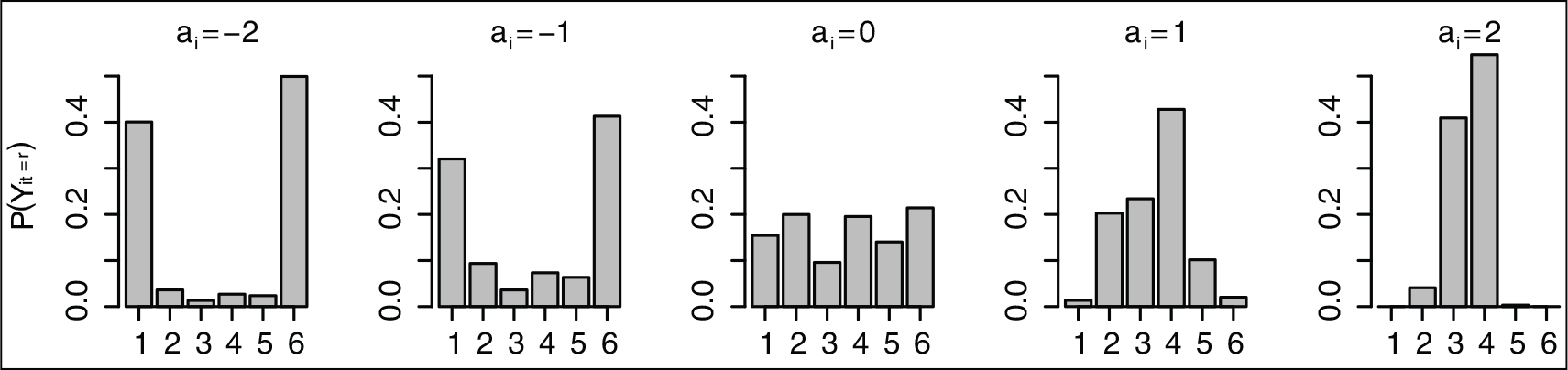
For

One obtains again
The parameter
Adjacent categories model
In the adjacent categories model, the intercept

that
Therefore, for adjacent categories models also, response style effects can be included by modifying the thresholds. The basic idea is to increase or decrease the difference between thresholds with a centring at the middle category (see also Tutz and Berger (2016)). In the predictor

where

The weights
Probabilities of single categories (for an example with
) depending on different values of response style parameter
in the adjacent categories model.
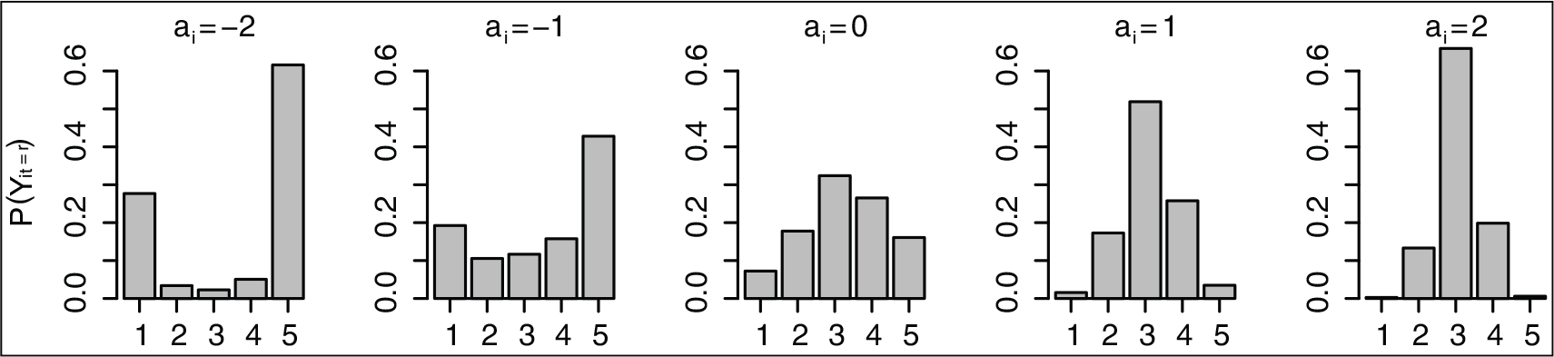
For illustration, let us consider two specific cases, both with an odd (
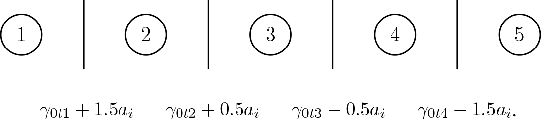
For

It should be noted that the modification of thresholds differs for the two types of models. In the cumulative model, the thresholds have to be ordered, therefore the subject-specific parameter modifies the difference between adjacent thresholds in a way that retains the order. The modification of differences between thresholds is multiplicative as is seen from equation (3.1). In the adjacent categories model, thresholds do not need to be ordered. Therefore, one can use a parameterization that changes the differences between thresholds in an additive way, see equation (3.2). The modification by adding subject-specific parameters has the advantage that one remains in the GLM framework, however, it can not be used for cumulative models. For cumulative models, an additive term
In the general model proposed here, the effect of explanatory variables is included by letting the parameters

In the cumulative model, one obtains (for k even)

The linear predictor is constructed by modifying the thresholds, which corresponds to the increase or decrease of differences between adjacent thresholds. The concept works for the cumulative and the adjacent-categories model. The corresponding models contain two effects, the location effect captured in
For

where
Let the data be given by
The model contains two random effects, the subject-specific intercept

where

where
For the adjacent categories model, one has

for the cumulative model, one has to build the differences
Simulation
A small simulation study is conducted to evaluate the performance of the method and the possible consequences of ignoring the response style. Before presenting the results, we first describe the general settings and the parameters that are used in the simulation scenarios.
Simulation settings
Per simulation,

while for the cumulative model the linear predictor in the DGP is defined as
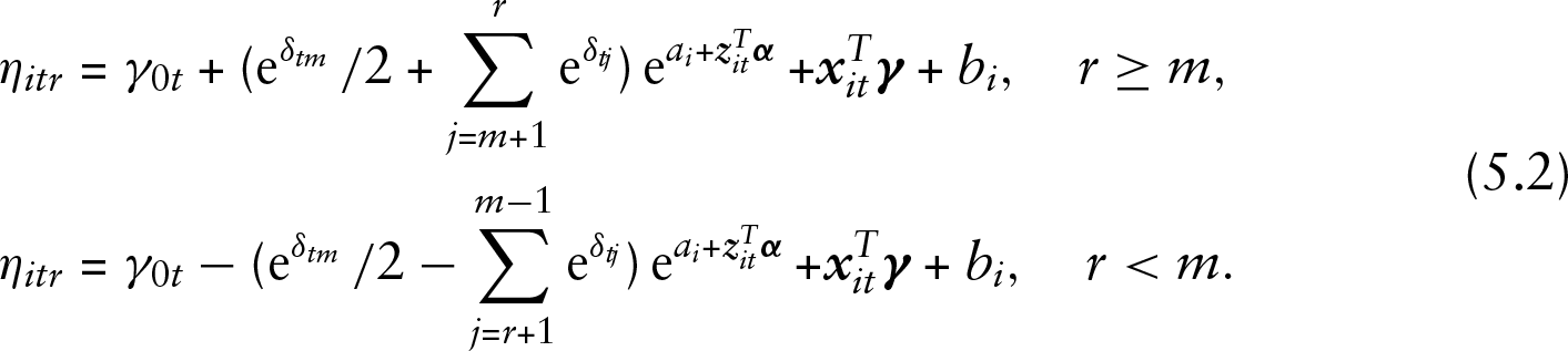
The explanatory variables contained in
The threshold parameters are set to fixed values. For the adjacent categories model, the matrix of the true threshold values is

while for the cumulative model the threshold parameters are

Two parameters are varied, namely the standard deviation of the random response style effect and the fixed response style effects corresponding to the explanatory variables. For the covariance matrix of the random effects

with three different effect strengths

For the response style effects
In total, these different values constitute nine different settings for the cumulative model and the adjacent categories model, respectively. These nine settings indicate different strengths of response styles, both for the response style caused by explanatory variables and caused by the random effects. Per setting, 100 replications are conducted. Each dataset is analysed with two different models: Model 1 (no RS) is a simple model without response style effects where the linear predictor is specified as
We are mainly interested in the fixed effects which are contained in both models, namely the threshold parameters
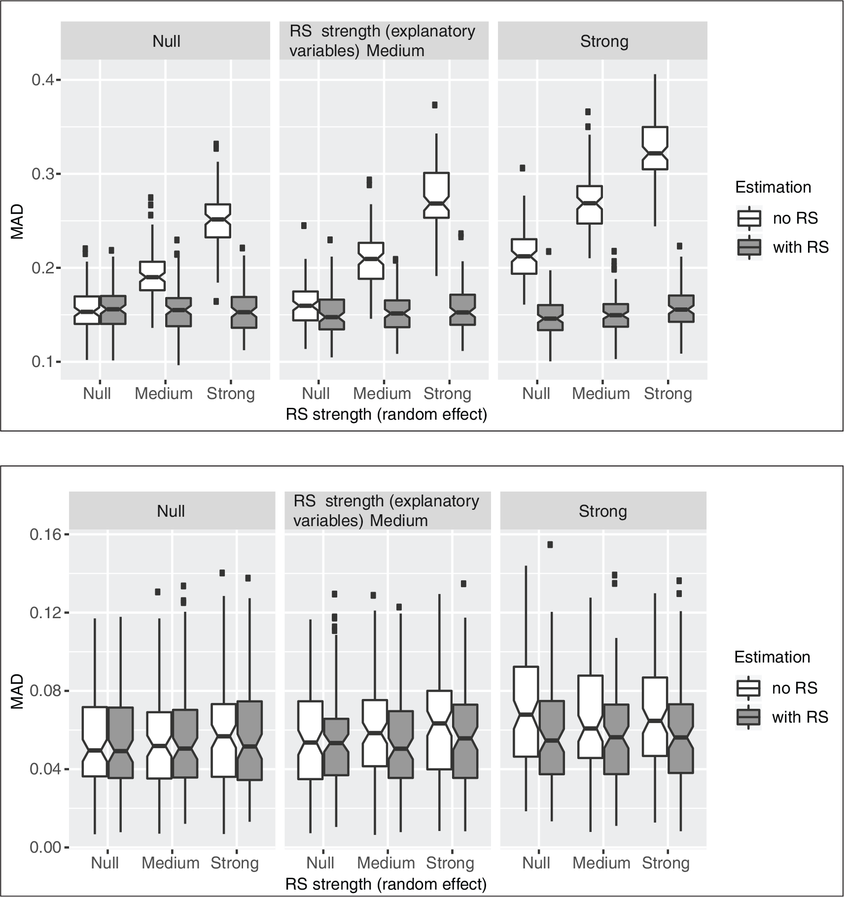
We distinguish between model 1 (no RS) and model 2 (with RS) by using different colours. With growing strength of the response style caused by the random effect and by the explanatory variables, the MAD of the parameters is growing when fitting model 1 while it remains rather constant for model 2. This effect is much stronger for the threshold parameters than for the covariate effects. This behaviour can probably be explained by the fact that the threshold parameters cover both the general location of the different responses as well as the general (i.e., not individual-specific) response styles across the studied population, while the covariate effects only cover location effects connected to
In the supplementary materials accompanying this manuscript, box plots for the estimates for each of the 40 threshold parameters can be found, separately for models 1 and 2, for the nine simulation setting, and for the adjacent categories model and the cumulative model. For the sake of simplicity, within this manuscript in Figure 5, we only present the respective results for the most extreme setting (with strong response style effects both for the random effects and the covariate effects) in the adjacent categories model. It can be seen that in model 2, the parameters are estimated unbiased, while the estimates in model 1 are severely biased in many cases.
Application to pre-election data
The method is applied to data from the GLES (Roßteutscher et al., 2017). The GLES is a long-term study of the German electoral process. It collects pre- and post-election data for several federal elections. The data we are using originate from the pre-election survey for the German federal election in 2017. In this specific part of the study, the participants were asked about specific political fears. More precisely, the participants were asked: ‘How afraid are you due to the...’
refugee crisis? global climate change? international terrorism? globalization? political developments in Turkey? use of nuclear energy?
The answers were measured on Likert scales from 1 (not afraid at all) to 7 (very afraid). As explanatory variables in the model we used:
The age of the participants ranges from 15 years to 94 years. The variable EastWest refers to the current place of residence where all Berlin residents are assigned to East Germany. For our analysis, the original dataset consisting of
Mean absolute deviation (MAD) for threshold parameters
(a) and for covariate parameters
(b) depending on the response style strength of the random effect and of the explanatory variables, separately for estimation with (black) and without (grey) response style effects in the adjacent categories model.

Mean absolute deviation (MAD) for threshold parameters
(a) and for covariate parameters
(b) depending on the response style strength of the random effect and of the explanatory variables, separately for estimation with (black) and without (grey) response style effects in the adjacent categories model.
Mean absolute deviation (MAD) for threshold parameters
(a) and for covariate parameters
(b) depending on the response style strength of the random effect and of the explanatory variables, separately for estimation with (black) and without (grey) response style effects in the cumulative model.
Parameter estimates separately for all threshold parameters in the simulation setting with strong response style effects both for the random effects and the covariate effects in the adjacent categories model. True values are marked with crosses.

(Standardized) parameter estimates (and p-values) for all covariate effects from models 1 and 2 (separately for the adjacent categories model and the cumulative model).
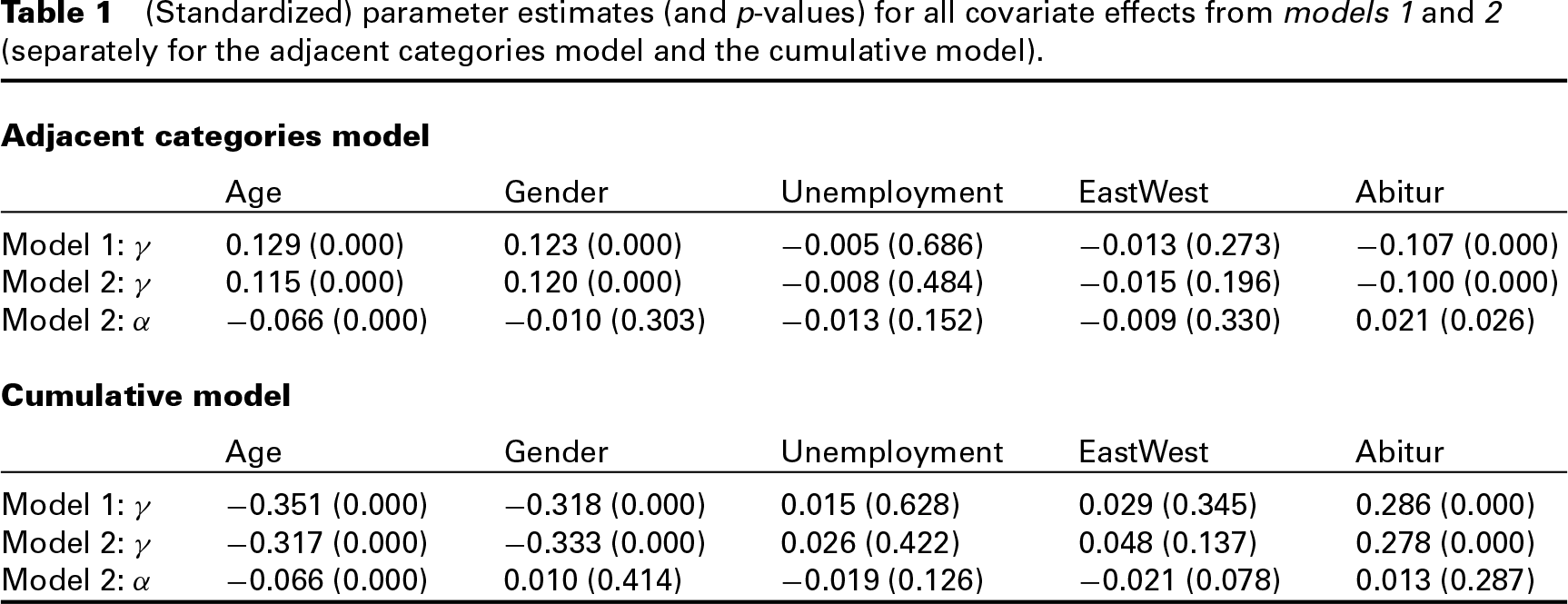
We fitted two different models, in model 1 possible response style effects (both the random effects and the covariate effects) are ignored, whereas they are included in model 2. For both models we used the adjacent categories approach as well as the cumulative modelling approach with logistic link. Table 1 shows the estimates of all covariate effects
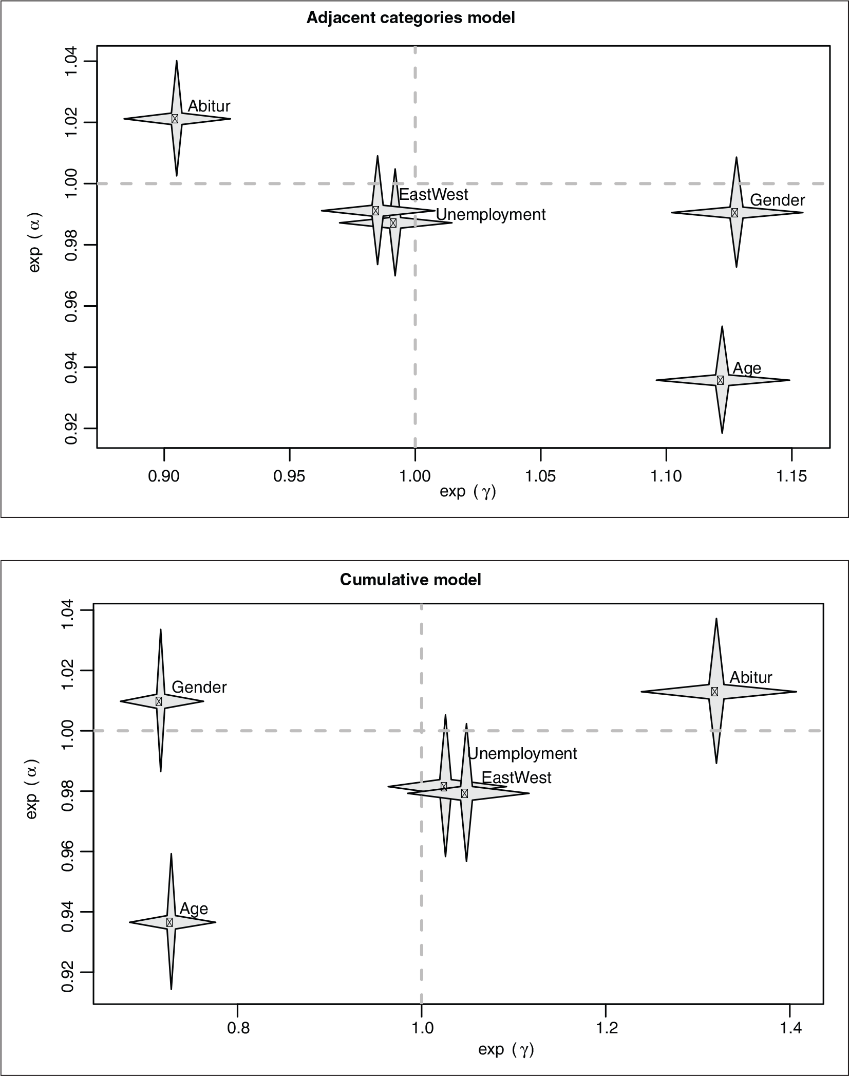
Figure 6 gives a visualization of the estimated effects and confidence intervals (a similar visualization tool was proposed by Tutz and Berger (2016)). It shows the exponentials of the covariate effects both for the location effects
It is immediately seen that location effects for Abitur, Age and Gender and the response style effect for Age are significant. In contrast to the cumulative model, in the adjacent categories model also Abitur has a significant response style effect. According to these estimates, the overall level of political fears is increased with increasing age and for women in comparison to men, while people with Abitur tend to have a lower level of fears than other respondents. On the other hand, with growing age people have an increasing tendency towards extreme categories, while people with Abitur show a tendency towards middle categories.
The random effects components are seen from the estimated (co-)variances for each of the models. For the adjacent categories models, we obtained 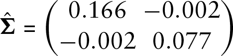
for model 2 with standard errors 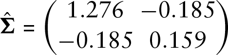
for model 2 with standard errors
(Exponential) effects of explanatory variables in GLES data together with 95% confidence intervals both for location effects
and response style effects
(separately for the adjacent categories model and the cumulative model).
We considered response styles for multivariate ordinal responses. Response styles may be present whenever individuals use rating scales, that can be an assessment of their own feelings or ratings that evaluate the performance of others. As has been demonstrated, ignoring response styles may yield inferior estimates of location effects. Therefore, one should check if they can be ignored or have to be included. Beyond the effect on the accuracy of estimates, response styles are of interest by themselves, in particular if explanatory variables are included. The modelling of the dependence of response styles on covariates shows which groups of respondents tend to more or less extreme responses.
The proposed models are implemented in an add-on package for
Footnotes
Supplementary materials
Supplementary materials for this article including more detailed results of the simulation studies are available from
Declaration of conflicting interests
The authors declared no potential conflicts of interest with respect to the research, authorship and/or publication of this article.
Funding
The authors received no financial support for the research, authorship and/or publication of this article.