
Abstract
Heterogeneity in response styles can affect the conclusions drawn from rating scale data. In particular, biased estimates can be expected if one ignores a tendency to middle categories or to extreme categories. An adjacent categories model is proposed that simultaneously models the content-related effects and the heterogeneity in response styles. By accounting for response styles, it provides a simple remedy for the bias that occurs if the response style is ignored. The model allows to include explanatory variables that have a content-related effect as well as an effect on the response style. A visualization tool is developed that makes the interpretation of effects easily accessible. The proposed model is embedded into the framework of multivariate generalized linear model, which entails that common estimation and inference tools can be used. Existing software can be used to fit the model, which makes it easy to apply.
1. Introduction
In behavioral research, rating scales have been used for a long time to investigate attitudes and behaviors. However, observed ratings may not represent the true opinion; in particular, response styles may affect the response behavior (see, e.g., Baumgartner and Steenkamp, 2001; Messick, 1991). An extensive overview on response styles in survey research was given more recently by Van Vaerenbergh and Thomas (2013). A response style is considered as a consistent pattern of responses that is independent of the content of a response (Johnson, 2003).
In the present article, we consider symmetric response categories of the form strongly disagree, moderately disagree, …, moderately agree, strongly agree and focus on response styles that are characterized by a disproportionate tendency to middle categories or to extreme categories, that is, the highest and lowest response categories. The preference to extreme categories is often called extreme response style and has been a topic of research for some time. Its counterpart, the tendency to choose middle categories, has been investigated, for example, by Baumgartner and Steenkamp (2001).
In many studies, the presence of response styles has been found. Response styles can differ, for example, across nations (Clarke, 2000; Van Herk, Poortinga, & Verhallen, 2004), ethnicity (Marin, Gamba, & Marin, 1992), or educational level (Meisenberg & Williams, 2008). In particular, in the psychometric literature, extreme response styles have been discussed within the framework of item response models. Bolt and Johnson (2009) and Bolt and Newton (2011) considered a multitrait model, which is a version of the nominal response model proposed by Bock (1972). Johnson (2003) considered a cumulative-type model for extreme response styles. Eid and Rauber (2000) considered a mixture of partial credit models that are able to detect response styles. More recently, tree-type approaches have been proposed. They typically assume a nested structure, where first a decision about the direction of the response and then about the strength is obtained. Models of this type have been proposed by Suh and Bolt (2010), De Boeck and Partchev (2012), Thissen-Roe and Thissen (2013), Jeon and De Boeck (2015), Böckenholt (2012), Khorramdel and von Davier (2014), and Plieninger and Meiser (2014).
In contrast to research in item response theory, where the focus is on the modeling of individual differences in terms of latent traits based on answers to several items without accounting for explanatory variables, we aim at investigating the influence of explanatory variables on the content-related choice and the response style for one item. The strength of the model is that it simultaneously accounts for both effects. Therefore, it allows us: to investigate content-related effects that are undisturbed by the response style for a single item, to investigate the response style undisturbed by content-related effects, to use covariates to disentangle content and style, and to avoid biased estimates of the content-related effects, which are the parameters of interest in most studies.
Approaches to simultaneous modeling of content-related effects and response styles seem to be scarce. Most approaches rely on the calculation of specific indices that can be corrected by regression techniques (see, e.g., Baumgartner and Steenkamp, 2001). An exception is the latent class approaches considered, for example, by Moors (2004), Kankaraš and Moors (2009), Moors (2010), and Van Rosmalen and Van Herk (2010). Latent class models are a strong tool, but specific software is necessary, and the existence of latent classes is always a strong assumption and interpretation has to rely on their existence. The crucial difference between these latent variable approaches and the proposed adjacent categories model is that the response style is not perceived as an individual trait but exists solely in relation to the covariates. The model does not need the additional assumptions that accompany latent variable modeling.
The proposed modeling of response styles generated by covariates for one item uses a concept of the response style that differs from the usual concept. In the psychometric literature, a response style typically is considered as a tendency in how a rating scale is used across items yielding a consistent pattern of responses that is independent of the content of a response (Johnson, 2003). When using this concept, multiple items are a necessity. In our approach, the tendency to extreme or middle categories is separated from the content-related effects by using the symmetry of the response categories and letting covariates determine the tendency to specific categories. Nevertheless, since the model provides an explicit modeling of a tendency to extreme or middle categories, the term response style seems also appropriate within our modeling framework.
In Section 2, the basic model is introduced. An illustrative example is given and a visualization tool is developed. In Section 3, the effects of parameters are discussed, and the potential bias of estimates is investigated. Section 4 is devoted to inference, and tools for the estimation of parameters are provided in Section 5. In Section 6, further applications that illustrate the method are given. In Section 7, we consider possible extensions and compare the approach to alternatives proposed, in particular, in item response theory.
2. An Extended Rating Scale Model
Let Yi ∈{1, … , k}, i = 1, … , n denote the observed responses on a rating scale; the categories 1, … , k represent graded agree–disagree attitudes with a natural symmetry like strongly disagree, moderately disagree, …, moderately agree, strongly agree. If the number of response categories is odd, there is a neutral middle category, and if k is even, there is none and the respondent is forced to exhibit at least a weak form of agreement or disagreement. Let xi denote a vector of explanatory variables that is observed together with the response Yi. Several models that link the explanatory variables to the ordinal response are available. Common model classes are the cumulative models, the sequential and adjacent categories models (see, e.g., Agresti, 2009; Tutz, 2012). We will focus on the adjacent categories model, which has the advantage that no constraints on the parameters are needed. Moreover, a specific version of the model is widely used in item response modeling. The so-called partial credit model (Masters, 1982) uses the adjacent logit link to model item difficulties but does not include explanatory variables. In the following, we first consider the basic model and then the extensions that account for response styles.
2.1. Adjacent Categories Model
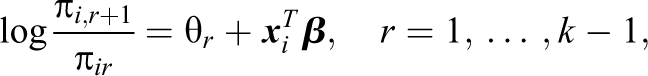
The model proposed here is an extension of the adjacent categories model. The basic form of the model with logit link is given by:
where π
ir
= P(Yi = r|
The interpretation of the parameters of the model is seen best when the parameters are given as functions of probabilities. For covariate vector

where π
r
(xj) denotes the probability of response category r for the vector of explanatory variables with the jth covariate having value xj, and π
r
(xj + 1) is the probability of response category r if the jth covariate is increased by one unit to xj = 1; all other variables are fixed. Thus,
2.2. Accounting for Response Styles
For simplicity, let us first consider the case of three response categories, k = 3. Then the model is given by the two equations that specify

The parameter δ
i
specifies the response style. If δ
i
→ ∞, one obtains πi2 → 1, which means a strong tendency to the middle category. If δ
i
→ −∞, one obtains πi2 → 0, which means a strong tendency to the response Categories 1 and 3 corresponding to the extreme response style. It is important that the response style is separated from the preference represented by the linear term
The effect of the additional parameter is illustrated in Figure 1 for a univariate explanatory variable with β = 1. It is seen that a person with δ i = 2 has a stronger tendency to choose the middle category than a person with δ i = 0, whereas a person with δ i = −2 hardly uses the middle category. Although the numeric values change, the shapes of the response functions for Categories 1 and 3 are very similar for all values of δ i .
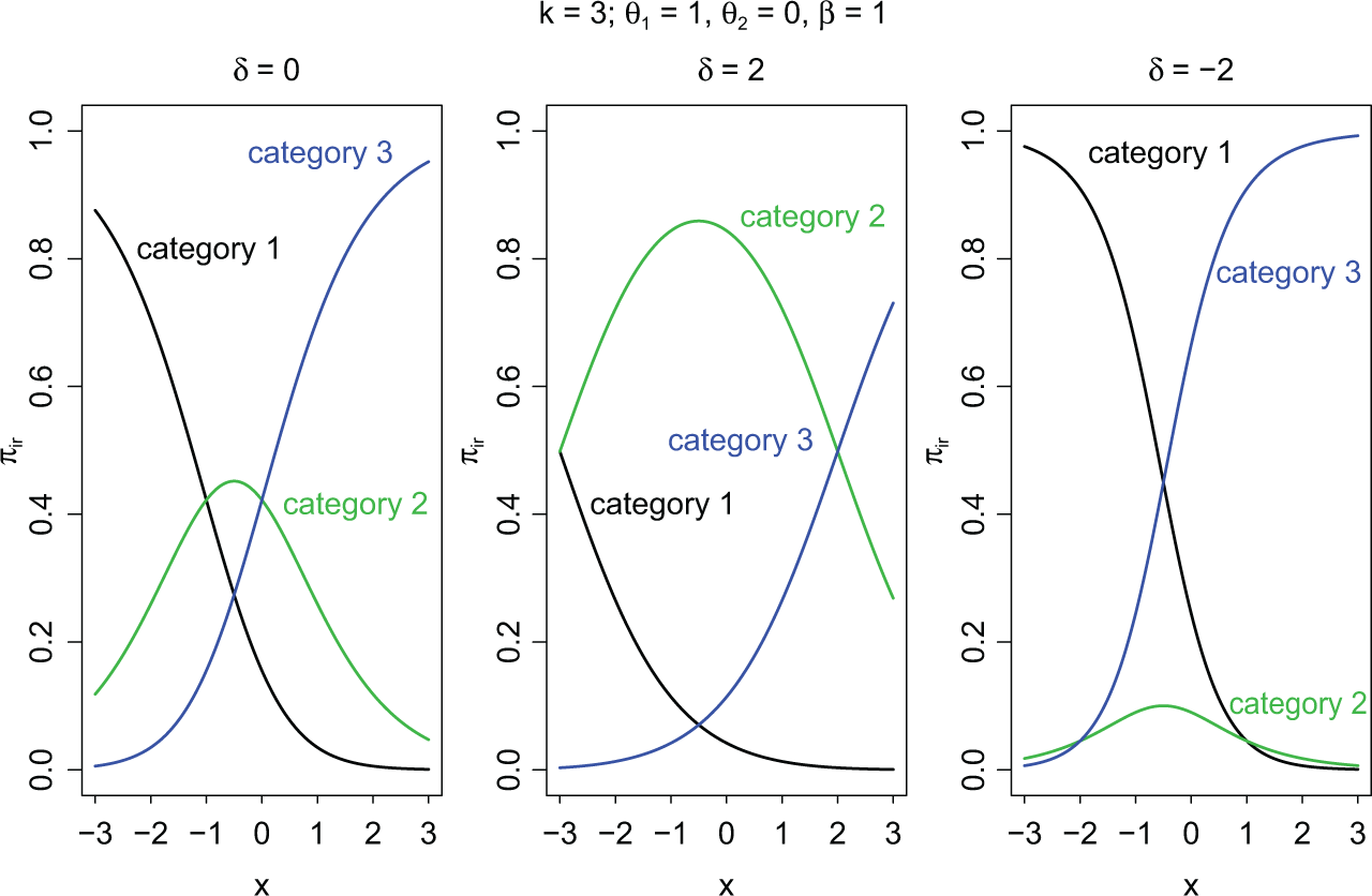
Response functions for several values of δ i .
The strength of the model is that the parameter δ
i
can be specified as a function of explanatory variables. Let

The model has some interesting properties. From:
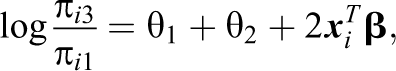
one sees that the log odds for the categories that actually represent agreement and disagreement are not affected by the term that determines the response style. On the other hand:
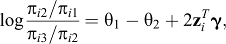
shows that specific odds ratios do not depend on the content-related term.
It is noteworthy that the parameters of the content-related term are the same as in the simple adjacent categories model. This may be seen from simple derivation of the parameters for the simple adjacent categories model. For three response categories, an even more intuitive form than Equation 1 is given by:
which shows the explicit dependence on the categories that refer to agreement or disagreement. For the parameters of the response-style effects, one obtains:
The explicit form of the parameters also ensures that the model is identifiable.
2.2.1. The general model for k response categories
In the general case, one has to distinguish between an odd and even number of response categories. For k odd, let m =[k/2] + 1 denote the middle category. Then the rating scale model that accounts for the tendency to the middle or extreme categories has the form:

The term
Positive values of the term
It should be noted that the modeling approach differs from alternative perspectives on response styles. In the literature, response styles are often defined as preferring the outer or the midpoint categories across many unrelated/weakly related items. In our model, a negative value of the response-style parameter indicating extreme response style captures not only a preference for the extremes “strongly agree” compared to the adjacent category “agree” but also a preference for “agree” compared to “somewhat agree.” The response-style γ parameter thus picks up not only the tendency to select the extremes but a general tendency to prefer more extreme categories, given the substantive stand of the respondent.
For k even, the model has a slightly different form. Let in this case m = k/2 denote the split between agreement and disagreement categories. Then the proposed model has the form:

The effect of the term
For simplicity, we will use the abbreviation RSRS for the model (k odd or even) for rating scale model accounting for response styles. Before discussing the effects in detail, we first consider an application.
2.2.2. An illustrative example
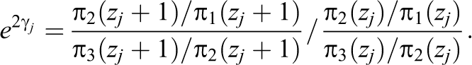
Although estimation methods have not yet been given, we consider an application to illustrate the effects obtained by using the extended model. We consider data from the Survey on Household Income and Wealth (SHIW) by the Bank of Italy that have been used before by Gambacorta and Iannario (2013). They are available from http://www.bancaditalia.it/statistiche/indcamp. The response is the happiness index indicating the overall life well-being measured on a Likert-type scale from 1 (very unhappy) to 10 (very happy). As explanatory variables, we consider gender (0 = male, 1 = female), the marital status (single, married, separated, and widowed), the place of living (north, south, and center), the general degree of confidence in other people from 1 (low) to 10 (high), the atmosphere the interview took place in (1–10), the citizenship, and the age in decades. The respondents were also asked about their assessment if the household income is sufficient to see the family through to the end of the month rated from 1 (with great difficulty) to 5 (very easily). The analysis is based on a subset with 3,816 respondents of the SHIW of 2010, age was centered around 60 and confidence around 5. We fitted a simple adjacent categories model with all of the covariates and the extended version that accounts for response styles, where all the variables are allowed to have content-related and response-style effects. For the variables age and confidence, we also included quadratic and cubic terms because the effects seem to be not negligible. First of all, it is interesting if the style-related effects are needed in the model. The likelihood ratio test for the null hypothesis H0 :
Parameter Estimates and Standard Errors for the SHIW Study
Note. SHIW = Survey on Household Income and Wealth.
2.2.3. Visualization of effects
The extended model contains more parameters than a simple rating scale model. In particular, when various explanatory variables are included, it is hard to keep track of all the relevant effects. Therefore, we provide some visualization tools to investigate the effect strength. We explicitly consider the case of an odd number of response categories (Model 2) and start with the visualization of linear effects. It is immediately seen that the odds of adjacent categories have the form:


where the explanatory variables for content-related effects have length p and the response-style effects length q. Thus, if the jth x variable increases by one unit, the multiplicative effect on the odds between adjacent categories is given by
If the jth z variable increases by one unit, the multiplicative effect on the odds between adjacent categories depends on the category. It is
For the SHIW study, we show the effects of the marital status, gender, and the area of living in Figure 2. In the figure, pointwise confidence intervals are included. We use stars with the horizontal and vertical lengths corresponding to the .95 confidence intervals of

Visualization of estimated effects for the Survey on Household Income and Wealth study including pointwise confidence intervals.
2.2.4. Visualization of nonlinear effects
In the example, the explanatory variables confidence and age contain in addition to linear terms quadratic and cubic terms. Then it is not sensible to plot the effects of parameters separately. One can understand the effects as functions of the corresponding explanatory variables. For example, the content-related effect of confidence is a polynomial containing cubic terms given by term


where
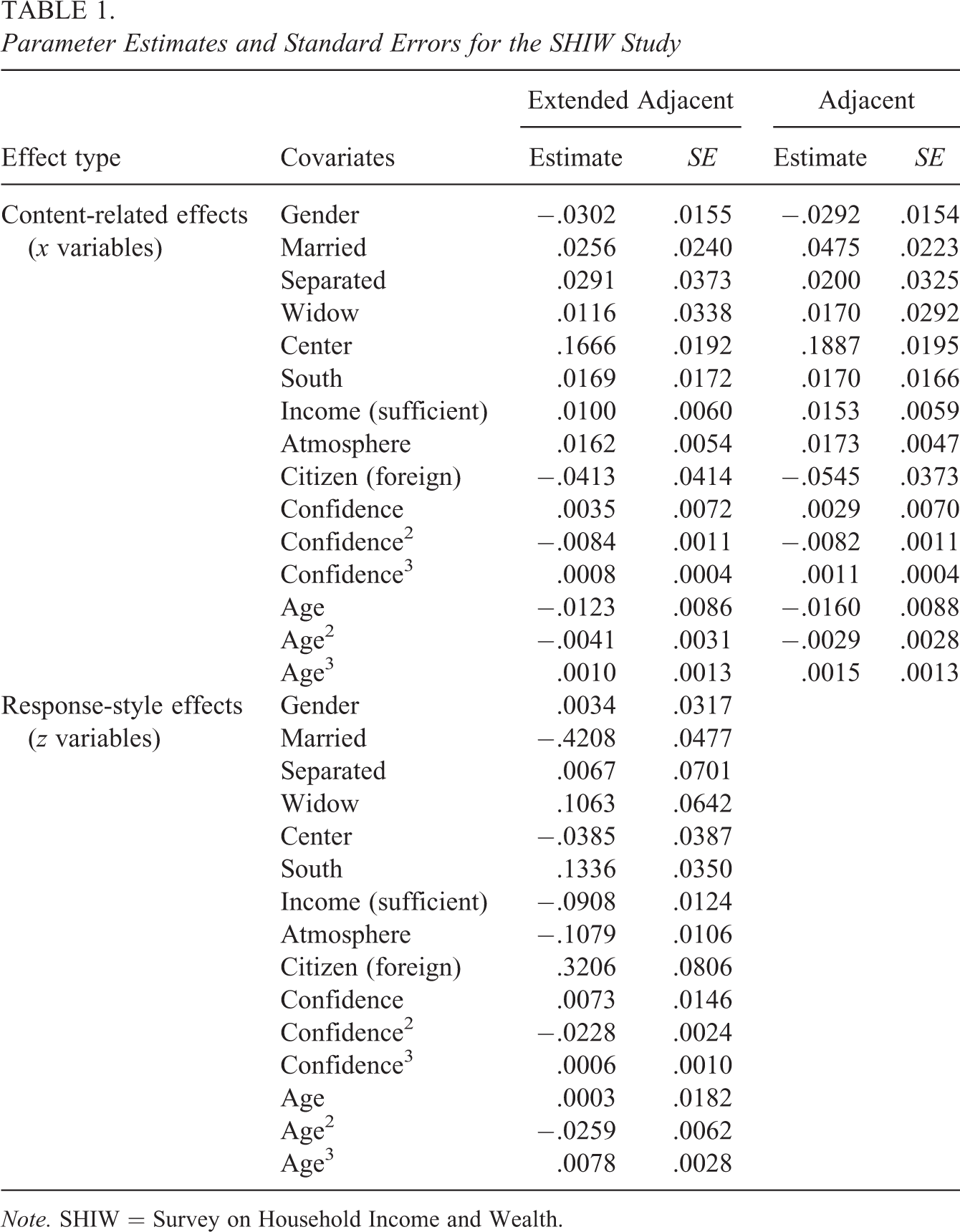
Parameters in polynomial terms are hard to interpret, but one can plot the corresponding nonlinear effects. Figure 3 shows the effects of content (first row) and response style (second row). In the plots we used the same scale in order to reveal the strength of the impact of the covariates. It is seen that with increasing confidence up to about value 5, the happiness increases and above 5 slightly decreases. For the response style, one gets a distinctly quadratic effect; the tendency to extreme categories (negative values of

Nonlinear effects of content and response style for confidence and age (Survey on Household Income and Wealth study); upper panels show the content and lower panels, the response-style effects.
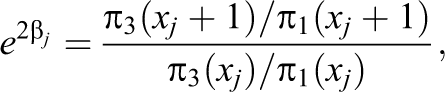
As an alternative to these conventional plots for nonlinear effects, we propose to visualize them in a similar way as for linear effects by using axes that correspond to effects of response style and effects of content. The corresponding plot is obtained for the covariate confidence by plotting
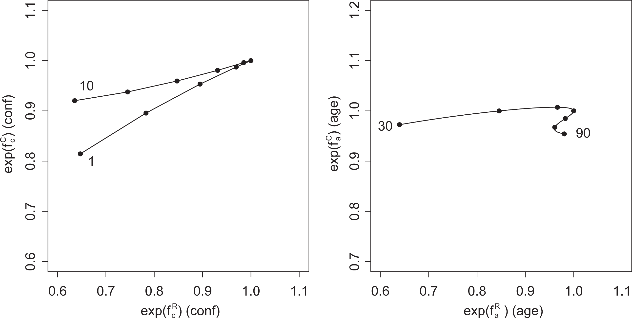
Curves for confidence (left) and age (right) for Survey on Household Income and Wealth study.
3. Effects in the RSRS Model
One of the strengths of the extended RSRS model is that the content-related effects are separated from the tendency to middle or extreme categories. We will investigate the separation for the case k odd; for k even the separation works in a similar way.
Let the model be given by Equation 2 and again m =[k/2] + 1 denote the middle category. Then one may derive that the parameters of the x variables are determined by:

where π r (xj) again denotes the probability of response category r for the vector of explanatory variables with the jth covariate having value xj and π r (xj + 1) is the probability of response category r if the jth covariate is increased by one unit to xj + 1; all other covariates are fixed. The representation (Equation 4) compares the probabilities for the categories m + r and m − r, that means categories with equal distance to the middle category. For k = 7 and therefore m = 4, it compares the probabilities of Categories 5 and 3, 6 and 2, and 7 and 1. Thus, it shows the effect of the explanatory variable in a symmetric way, namely, how strong is the preference of, for example, Category 5 compared to 3 if the explanatory variable increases by one unit.
It is essential that the parameter β
j
does not depend on the term
For the parameters that determine the response style, one obtains:

where in a similar way as before π
r
(zj) denotes the probability of response category r for the vector of explanatory variables with jth covariate zj and π
r
(zj + 1) is the probability of response category r if the jth covariate is increased by one unit to zj + 1; all other covariates are fixed. The parameter γ
j
depends only on response probabilities of categories m, m + r, and m − r for different values of zj. It represents how the concentration of the probability mass is increased in the middle if zj is increased by one unit. In the same way as β
j
is separated from

Estimates for several values of β,γ and samples sizes: Explanatory variable follows a standard normal distribution, the true values are given in gray.
3.1. Accuracy of Estimates if the Response Style is Ignored
If one is not aware of response styles, one fits a regression model that contains only the effect of explanatory variables on the response. In the following, it is demonstrated that this procedure can result in strongly biased estimates and poor accuracy of the estimates of
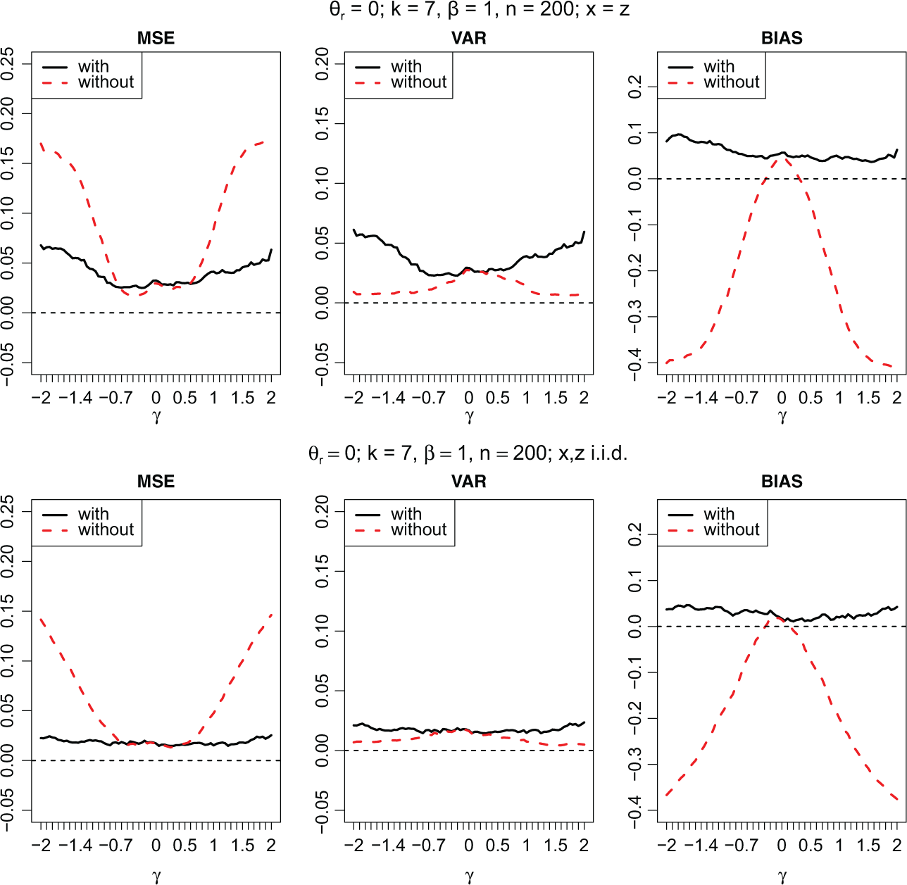
Mean squared errors, variances, and bias as a function of γ; in the upper panel, one has x = z, and in the lower panel, x and z differ and are independent. Dashed lines indicate the model without accounting for the response style, and the drawn lines indicate the model with response-style effects.
One might suspect that the bias is so strong because the variable has two effects, one on the preference and one on the response style. Therefore, we also investigated the case with a predictor η r = θ r + xβ + zγ, where x,z are independently normally distributed variables. The lower panel of Figure 6 shows the resulting curves. It is seen that one obtains biased estimates also if a variable that is independent of x generates varying response styles but is ignored. Therefore, one ignores heterogeneity of response styles in the population.
In Figure 6, the effect is always attenuation of effects, a familiar phenomenon that also occurs in random effects models if heterogeneity is ignored (see, e.g., Tutz, 2012, Chapter 14). However, in the case of ignored response styles in some cases, one can also see stronger effects. In Figure 7, MSE, bias, and variance are shown for the same models as in Figure 6, but now the thresholds have been changed to θ1 = 0, θ2 = −0.4, θ3 = −0.8, …. For these thresholds, higher categories are preferred for all of the values of the explanatory variables. It is seen that the bias is again negative for all values of γ if x and z are uncorrelated (lower panel), but one obtains overestimation of the true value of β = 1 in the case where x = z if γ is positive (upper panel). Therefore, if there is a tendency to higher categories and the effect β is positive, and one ignores the tendency to select middle categories (γ positive), this is interpreted by the model without response effect as a stronger β. The consequence is that larger values of β are obtained, the estimated effect tends to be larger than the true effect. The same effects are also found if more than just two variables are included in the model. For illustration of the effects, we considered values of γ from a wide range. Although large values of γ might occur, in the real data sets we considered |γ| was not beyond 1. An indicator of potential nonnegligible bias might be strong differences in estimates for the model with response style and the model without response style.
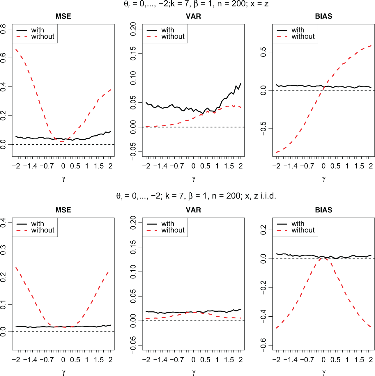
Mean squared errors, variances, and bias as a function of γ; in the upper panel, one has x = z, and in the lower panel, x and z differ and are independent. Dashed lines indicate the model without accounting for the response style, and the drawn lines indicate the model with response-style effects.
3.2. Effect of Sample Sizes
It has been demonstrated that biased estimates can be avoided by accounting for the response style when estimating the content-related effects. A quite different question is which observations contribute to the estimation accuracy when differing response styles are present and accounted for in the model. Intuitively accuracy of estimates will be weaker if many respondents prefer the middle category because then there is a tendency that less information about
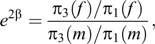
where π
r
(f), π
r
(m) denote the probability of an response in category r for females and males, respectively. If in one of the two populations there is a strong tendency to the middle categories, the relative frequencies corresponding to π3(⋅)/π1(⋅) will be estimated very unstable because only few observations will be observed in Categories 1 and 3. Consequently, the accuracy of
To demonstrate the effect, we show simulation results. We consider a binary predictor x ∈ {0,1} and effect strengths β = 1 and γ = 1. Figure 8 shows the MSEs for a range of sample sizes, where n0 denotes the sample size of population x = 0 and n1 the sample size of population x = 1. In the left panel, the thresholds were θ1 = θ2 = 0 yielding probability vectors (0.33, 0.33, 0.33) for x = 0 and (0.06, 0.468, 0.468) for x = 1. Therefore, in the population x = 1, the proportion π3(x = 1)/π1(x = 1) is rather extreme and unstable to estimate. It is seen from Figure 8 that increasing the number of observations in the population x = 0 does improve estimation accuracy only very little, while increasing the number of observations in the population x = 1 improves the estimation accuracy very strongly. In the right panel of Figure 8, the thresholds are θ1 = −2, θ2 = 0 yielding probability vectors (0.787, 0.106, 0.106) for x = 0 and (0.33, 0.33, 0.33) for x = 1. Now the proportion π3(x = 0)/π1(x = 0) is rather extreme and unstable to estimate. As is seen from the right panel, increasing the number of observations in the population x = 0 strongly improves the estimates, while increasing the number of observations in the population x = 1 hardly matters.
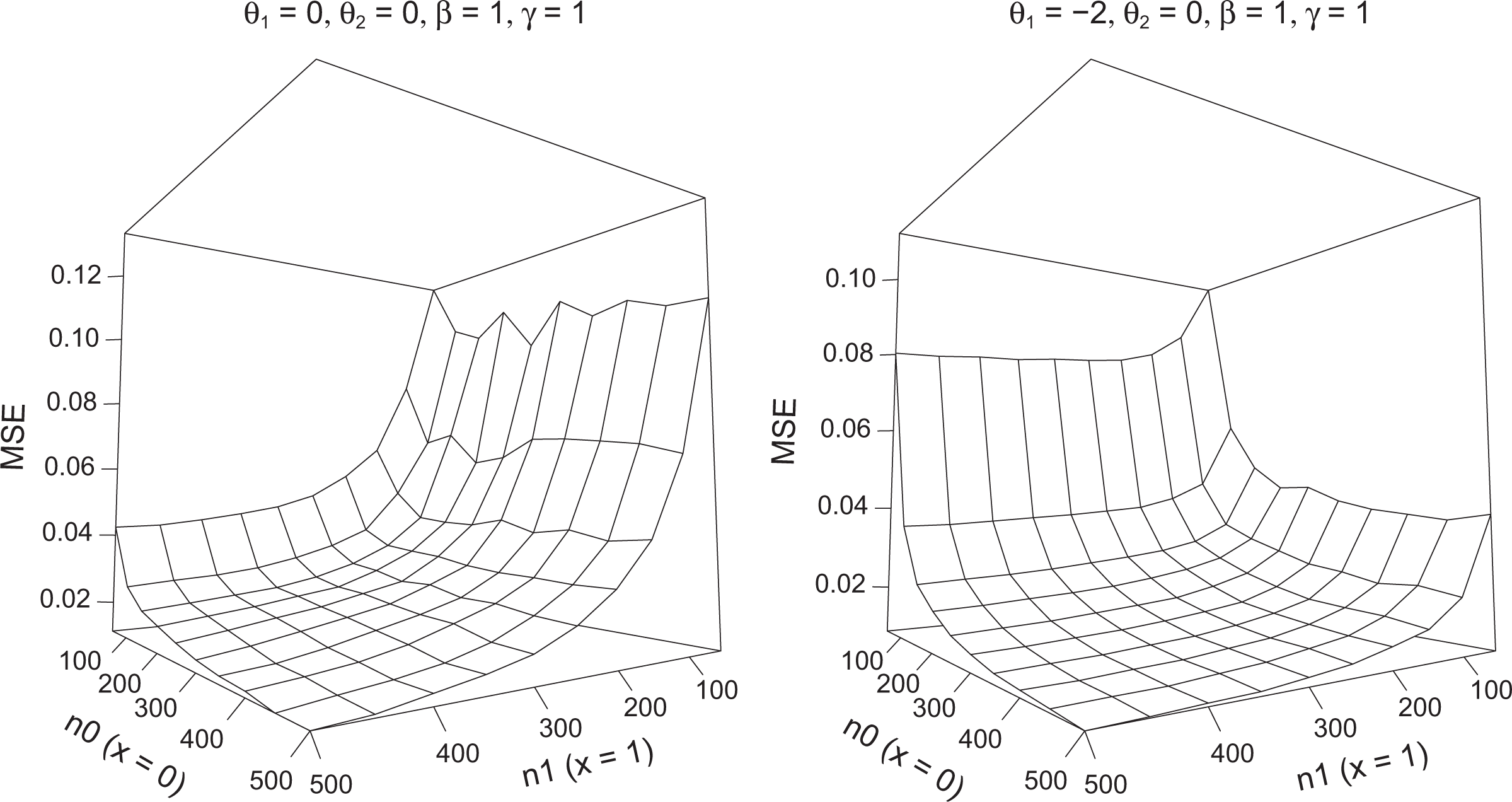
Mean squared error as a function of the sample sizes n 0, n 1 for subpopulations x = 0, x = 1, respectively.
Thus, if extreme proportions occur in one population, which can be induced by response styles, estimation accuracy profits from the increase in these populations. The effect cannot be exploited in a first investigation, but if one has a pilot study, which gives first results on the probabilities to expect, it can be used to stratify the sample in future studies to improve the accuracy of estimates.
4. Estimation of Parameters and Inference
Estimation and testing of the model is simplified by embedding the model into the framework of (multivariate) generalized linear models (GLMs). Let the data be given by (

where
An equivalent form of the link between explanatory variables and response is:

where h = (h1, … , hk−1) = g−1 is the so-called response function. Equations 5 and 6 represent the structural assumption of a multivariate GLM. Maximum likelihood estimates and inference for multivariate GLMs are extensively discussed in Fahrmeir and Tutz (2001) and Tutz (2012). For example, one can use likelihood ratio tests, score tests, or Wald tests to test linear hypotheses of the form H0 :
An interesting aspect is the covariance of estimates which is asymptotically given by the expected information or Fisher matrix,
The blocks
5. Implementation and Available Programs
The model can be estimated and evaluated by using the flexible R-package vector generalized linear and additive model (VGAM; Yee, 2010, 2014), which also has to be used in estimation and testing of our applications.
6. Further Applications
6.1. Health Care
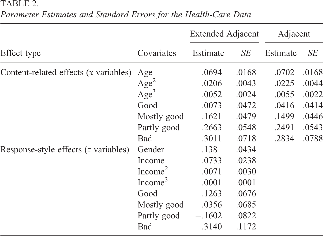
As a second application, we use data from the ALLBUS, the general social survey of social science carried out by the German institute GESIS. They are available from http://www.gesis.org/allbus. For our analysis, we consider data from 2012 consisting of 2,899 persons. The response is the confidence in the health-care system measured on a scale from 1 (no confidence at all) to 7 (excessive confidence). Explanatory variables that we include in our model are gender (0 = male, 1 = female), income in thousands of euro, age in decades, and the medical condition of the person on a scale from 1 (very good) to 5 (bad). Again we estimated a simple adjacent categories model and the extended model, where all covariates were allowed to have content-related and response-style effect. In a second step, we refitted the model including only the covariates with a significant effect in each part. The estimated coefficients and the corresponding standard errors are given in Table 2. Concerning variable selection, covariate gender and income are excluded from the x variables, and covariate age is excluded from the z variables. The likelihood ratio test statistic for the global hypothesis H0 :
Parameter Estimates and Standard Errors for the Health-Care Data
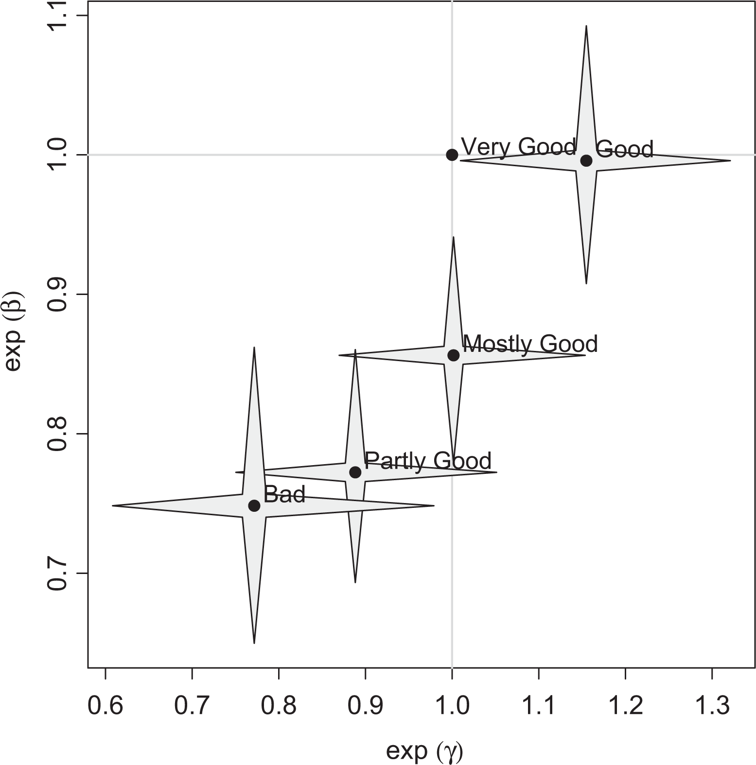
Visualization of estimated effects of covariate medical condition for the health-care data.

Nonlinear effects of content and response style for income and age (health care); upper panels show the content and lower panels, the response-style effects.
6.2. Motivation of Students
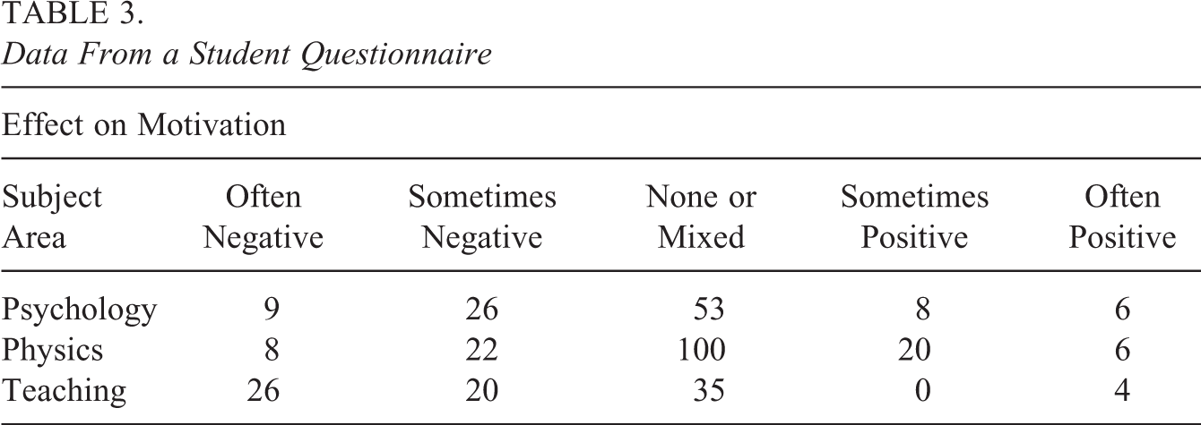
As a third example, we consider data from a student questionnaire. It has been evaluated what effect the expectation of students for getting an appropriate job has on their motivation. The response is the effect on motivation on a scale from 1 (often negative) to 5 (often positive), with intermediate values “sometimes negative/positive” and no effect. For our analysis, we use data from 343 students from the subject areas psychology, physics, and teaching serving as explanatory variable. The data are given in Table 3. Overall there is a strong preference for the middle categories, which is characteristic for this sort of question. The comparison of the simple adjacent categories model and the extended model yields the likelihood ratio test statistic 6.14 on 2 degrees of freedom. Thus, response-style effects again should not be neglected. The estimated coefficients for both models are given in Table 4, a visualization of the effects of the extended model including pointwise confidence intervals is shown in Figure 11, where subject teaching was chosen as reference category.
Data From a Student Questionnaire
Parameter Estimates and Standard Errors for the Student Questionnaire

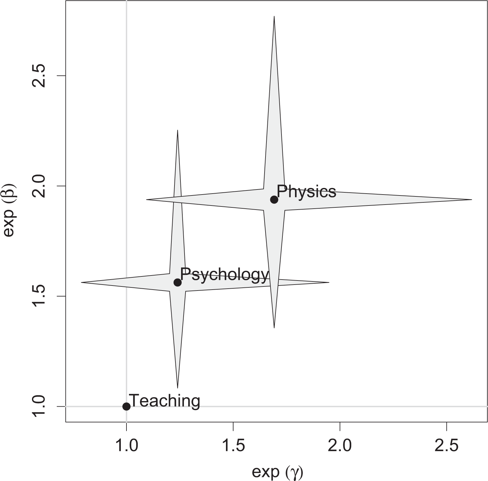
Visualization of estimated effects of covariate subject area for the student questionnaire.
The estimates in the content-related part of the model show that students of psychology and physics see more positive effects on their motivation than students of the teaching profession. In fact, job prospects for students of the teaching profession are poor nowadays. The estimated response-style effects show a significant tendency to middle categories for students of physics as compared to students of the teaching profession.
A comparison of the content-related effects in Table 4 for the simple and the extended model shows that the estimates of the simple model are considerably larger. Thus, one observes a positive bias in the estimated β coefficients of the x variables when ignoring response-style effects. One reason for the positive bias is the peculiar distribution of the data. Table 3 shows that most observations are in the middle category (none or mixed), and at the same time, there is a general shift to the left or to low categories. Therefore, ignoring the tendency to the middle category leads to an overestimation of the β coefficients.
7. Extensions and Comparison With Alternative Approaches
In the following, we shortly sketch possible extensions of the modeling approach. The first concerns the handling of nonlinear effects. If one has continuous covariates, one can replace the linear term
The model considered here by construction disentangles the effects of response style and content for 1 item. The basic concept to include a subject-specific term (added for response categories r = 1, … , m − 1 and subtracted for categories r = m, … , k − 1 if k is odd) can also be used when one wants to model the response style for more than 1 item. The additional effect can be a simple subject-specific effect, representing heterogeneity of persons, or can depend on covariates in the way as specified here. Then one obtains a specific extended partial credit model that accounts for response styles. Although the extension is straightforward as a model, the estimation procedures used here might not be the best choice. In a partial credit model that accounts for the response style in the way proposed here, one has to estimate the item difficulties, the person abilities, and the additional response-style parameters, either as subject-specific parameters or as depending on covariates or both. If one uses just a linear term depending on covariates (and no subject-specific response-style parameter) the proposed estimation procedure can directly be used. However, it is certainly more attractive to model the heterogeneity by including an own subject-specific response-style parameter, for example, as a random effect. The modeling as random effect allows to reduce the number of structural parameters to estimate since one has only to estimate the variance of the random effects. However, then specific estimation procedures for the maximization of the marginal likelihood are needed and have to be developed. An additional problem is that the response style might depend on the item. The assumption that it is the same for all items is rather strong. If one lets it depend on items, one gets an inflation of parameters that call for regularization techniques or other novel estimation techniques. The extended partial credit model is certainly worth investigating, but the investigation of the possible models and the development of appropriate estimation tools need further research that is beyond the scope of the present article.
Nevertheless, we will shortly consider the differences of the method used here and some of the modeling approaches to response styles that have been proposed, in particular, in item response theory. A traditional way to account for differences in the use of rating scales are mixture models. For example, Eid and Rauber (2000) investigated measurement invariance in organizational surveys by using the polytomous mixed Rasch model. The basic assumption is that the whole population can be subdivided into disjunctive latent classes yielding parameters that are linked to the classes. Typically one fits models with two or three classes obtaining class-specific parameters that have to be interpreted. As Eid and Rauber (2000) demonstrated, when fitting a model with two latent classes, the classes might represent different response styles. The main difference to the approach propagated here is that response styles are not explicitly modeled. The resulting classes can represent extreme response styles or a tendency to the middle categories but do not have to. It might occur that no specific pattern referring to response styles is found for the latent classes. Although finite mixture models are an interesting approach to model heterogeneity, in particular, the number of latent classes is not so easy to determine, and if one fits a model with more classes, one might obtain quite different estimates and therefore different interpretations. Similar problems are found for the class of multidimensional extensions of response models that account for response styles as considered, for example, by Bolt and Johnson (2009). By including further latent traits in the predictor, one obtains multidimensional models. The additional traits can represent response styles. Again the difference is that response styles are not explicitly searched for. Of course, one might see this as an advantage. However, there is again some arbitrariness concerning the number of latent traits and the interpretation. The arbitrariness is augmented if the estimates have to be rotated (see, e.g., Bolt & Johnson, 2009) to obtain a simple interpretation. If one suspects different response styles, we find it more attractive to model them explicitly. If one accounts for them by construction, one can see if they are present or not.
More explicit modeling of response styles is found in tree-type models as considered, for example, by Thissen-Roe and Thissen (2013) and more recently by Jeon and De Boeck (2015). The models assume a sequential decision model. In a first stage, it is distinguished between a positive and a negative response, and in subsequent steps, the strength of the response is determined. Models of this type can be seen more general as nested models (Suh & Bolt, 2010). For ordinal responses with covariates, they have been used earlier by Tutz (1989). The models are similar in spirit to the approach proposed here; they model response styles by parameters and have to distinguish between odd and even number of categories. The main differences are in the sequential decision procedure and the parameterization. In step models, one assumes 1PL or 2PL models for the separate steps. In the approach considered here, there is no sequential mechanism assumed, and the parameters are embedded into an adjacent categories model.
Finally, we want to mention approaches to validate the interpretation of response style. In the case of several items, this may be done by either selecting 2 item subsets that are weakly or unrelated (Moors, 2003, 2004) or using many items (Johnson, 2003; Van Herk et al., 2004) that are unrelated (Baumgartner & Steenkamp, 2001; Clarke III, 2001; Weijters, Cabooter, & Schillewaert, 2010). This allows researchers to be certain that a persistent tendency across unrelated items can be ascribed to style (unrelated to item content). In our approach, only 1 item is used to detect response styles, but the model is constructed in a way to pick up the response style linked to the particular question that is asked.
8. Concluding Remarks
A model is proposed that simultaneously accounts for content-related effects and response styles that have a tendency to middle or extreme categories. Thus, content-related effects can be studied without being influenced by the presence of specific response styles and vice versa. In traditional ways to investigate extreme response styles, for example, by computing an index for extreme response styles as the relative number of scores given on the extreme categories as used among others by Bachman and O’Malley (1984) and Van Herk, Poortinga, and Verhallen (2004), it is not known how the content-related effects are linked to the index. This is avoided by simultaneous modeling.
A particular strength of the approach is that it provides an easy-to-use tool and may avoid biased estimates. Of course, it cannot solve all the problems connected to rating scales. For example, it does not address problems linked to the number of response categories and response category labels (Weijters et al., 2010) or the tendency to show greater acquiescence (Baumgartner & Steenkamp, 2001) but can ameliorate some of the effects that come with specific response styles. Since researchers should “do whatever they can to control for response styles” (Van Vaerenbergh & Thomas, 2013), an easy-to-use tool should also be used.
Footnotes
Acknowledgments
We thank three reviewers and the coeditor for their constructive comments which helped to improve the article considerably.
Declaration of Conflicting Interests
The author(s) declared no potential conflicts of interest with respect to the research, authorship, and/or publication of this article.
Funding
The author(s) received no financial support for the research, authorship, and/or publication of this article.
References
Supplementary Material
Please find the following supplemental material available below.
For Open Access articles published under a Creative Commons License, all supplemental material carries the same license as the article it is associated with.
For non-Open Access articles published, all supplemental material carries a non-exclusive license, and permission requests for re-use of supplemental material or any part of supplemental material shall be sent directly to the copyright owner as specified in the copyright notice associated with the article.