Rethinking the Normal Vote,the Personal Vote,and the Impact of Legislative Professionalism in U.S. State Legislative Elections

Abstract

Legislators might rely on their partisan base for electoral support—what scholars call their normal vote—or they may cultivate support among nonpartisans through casework or constituency service—what scholars call a personal vote. Previous research frequently argues that legislators face a tradeoff between pursuing the normal vote and a personal vote as traditionally defined, often focusing on resources used by incumbents to build their personal vote. In contrast, we argue that securing the support of partisans and nonpartisans alike should be evaluated based on how a legislator performs in office, and that the so-called normal and personal vote need not be viewed as in conflict. We evaluate our claims using data from state legislative elections following redistricting, focusing on legislative professionalism to measure the resources available to incumbents that they might use to cultivate a personal note.

Keywords

elections political behavior representation legislative elections legislative politics legislative professionalism redistricting

The electoral connection between legislators and their constituents defines representation in democracies.¹ The existing literature has offered two key concepts that help explain this connection: the normal vote and the personal vote. As traditionally defined, the normal vote refers to the electoral support an incumbent could expect to receive based on the underlying distribution of partisanship in her district. In contrast, the personal vote refers to the electoral support received by incumbents from voters who are not members of her party, but who respond positively to some other aspect of the incumbent’s performance while in office. In describing these two features of legislative elections, scholars frequently assert two claims: (a) that legislators face a trade-off in seeking to secure their normal vote versus pursuing a personal vote, and (b) that the resources available to legislators seeking reelection help them pursue a personal vote. In this article, we argue for a reformulation of these concepts.

Specifically, we argue that performance in office should affect the level of support incumbents receive from both voters who are members of their party and voters who are not. Making performance in office the central feature of support from both groups of voters transforms the potential trade-off in support among voters in each group from a theoretical assumption to an empirical question. Similarly, it also becomes an empirical question regarding whether the resources available to incumbents are limited only to expanding their support among voters who are not members of their party. The result is a more general theory of incumbent pursuit of reelection that makes fewer assumptions and presents a broader range of testable propositions.

We evaluate our reformulation using data from 1,610 state legislative contests taken from 41 states in 2002 after legislative redistricting took place. Like Ansolabehere, Snyder, and Stewart (2000) and Desposato and Petrocik (2003), we study elections following redistricting because it allows us to compare the electoral support received by incumbent legislators in the new portions of their districts added after redistricting to their electoral support in the older portions of their districts that were retained. This allows us to isolate the electoral support an incumbent gains through performance in office, including service to the district, because voters in the old part of an incumbent’s district have experienced the incumbent’s performance, but those in the new portion of the district have not. Finally, we examine how differences in legislative professionalism affect the patterns of electoral support incumbents receive in the old and new portions of their districts from voters in their party and voters not in their party.

The Normal Vote and the Personal Vote

Converse (1966, 14) defines the normal vote as the “long-term component [of voting that] is a simple reflection of the distribution of underlying party loyalties.” In other words, the normal vote is the share of the vote a candidate can expect to receive simply based on partisanship. Converse (1966) rests this idea on a micro-level view of party identification as durable, stable, and a key predictor of vote choice for citizens. This follows the more general assertion that party identification represents a deeply held attachment for voters (e.g., Campbell et al. 1960).

Cain, Ferejohn, and Fiorina (1987, 9) define the personal vote as, “. . . that portion of a candidate’s electoral support which originates in his or her personal qualities, qualifications, activities, and record.” This has generally been viewed as based on nonideological behavior such as casework, credit claiming, and bringing so-called “pork barrel” benefits back to the district (e.g., Ansolabehere, Snyder, and Stewart 2000; Fiorina 1977; Mayhew 1974). Such behaviors are consistent with aspects of Fenno’s (1978) description of what he calls homestyle. Numerous scholars point to the personal vote as the primary source of advantage incumbents enjoy in their reelection bids (e.g., Desposato and Petrocik 2003; Jacobson 2004), sometimes treating the personal vote and incumbency advantage as synonyms.

Thus, the electorate can be divided into two groups: (a) those normally inclined to vote for candidates of the incumbent’s party, and (b) those normally inclined to vote for candidates from the other party. The existing literature views the normal vote as support received from the first group, while the personal vote refers to support received from the second group. For some scholars, the personal vote is viewed as additional support incumbents can gain independent of the normal vote they should expect due to partisanship (e.g., Jacobson 2004; Mayhew 1974). In fact, Mayhew (1974, 26) states that incumbents, “. . . can—indeed must—build a power base that is substantially independent of party.”

In contrast, some argue that legislators face a trade-off between the support they receive from the normal vote and support they receive from the personal vote. This constitutes a very different understanding of what the normal vote is. To assume that the normal vote is involved in any sort of trade-off implies that incumbents cannot necessarily take the support of their partisan base for granted.² Fiorina (1977) argues that focusing attention on constituency service and casework by members of Congress weakens the partisan connection between voters and their representatives. While Fenno (1978) reports some examples of members of Congress who develop a homestyle based on their policy decisions, he presents many more examples of members developing a homestyle based on nonpolicy factors. Finally, Ansolabehere, Snyder, and Stewart (2000, 27) report evidence they argue supports the claim that, at least since the 1960s, the emergence of “. . . the personal vote acts against party strength.” They go on to say, “The substitution of the personal vote for the party vote . . . suggests that the personal vote erodes partisan attachments,” and that it reflects the “trade” made by legislators as they balance their need to toe the party line in some instances with their need to appease voters who do not share their partisan leanings (p. 31).

Thus, the existing literature is unclear regarding how these two concepts relate to each other, including some prominent scholars who have suggested support for both views in the same piece (e.g., Mayhew 1974). We see no need to assume whether or not there is a trade-off between these two sources of electoral support—we see it best left as an empirical question. If pursuit of a personal vote among constituents who did not share a legislator’s party affiliation required that legislator to moderate her policy positions, then the logic of a simple proximity-based spatial model (e.g., Downs 1957; Enelow and Hinich 1984) would suggest a trade-off between the personal vote and the normal vote. As a legislator moved her location in the issue space to attract new voters, she would risk losing some portion of her current (partisan) base.³

However, the personal vote is generally thought to emerge in response to the nonideological behavior of the legislator. Casework, pork-barrel projects, and constituency service are presumed to be the main tools used to develop a personal vote—none of which require any change in the policy position of the legislator. As a result, legislators should be free to pursue the retention of support from their own party supporters via their location in the policy space while also building support among those not of their party through nonpolicy-related behavior.

Stated in more general terms, an incumbent’s performance can be evaluated in both ideological and nonideological terms. Furthermore, voters of the incumbent’s party and voters not of the incumbent’s party are free to evaluate the incumbent’s performance on both ideological and nonideological grounds. As a result, the support an incumbent receives from these two groups of voters may or may not be independent—it is an empirical question.

This assertion requires a careful consideration of what would constitute empirical evidence of a trade-off versus independence in support among these two groups of voters for the incumbent. Ansolabehere, Snyder, and Stewart (2000) argue that in an open-seat race, the presence of the normal vote should lead to a 1-to-1 translation between the normal share of the two-party vote a candidate receives in a district and the vote share a candidate actually receives. Thus, plotting the normal vote for Republicans(Democrats) on the X-axis of a graph and the actual vote share received by Republican(Democratic) candidates on the Y-axis should result in a 45-degree line with a slope of 1. This is illustrated in Figure 1 with a solid line. We present Figure 1 because scholars have interpreted a slope coefficient of less than 1 as an indication of a less than perfect link between the normal vote and election outcomes, suggesting a trade-off between the personal vote and the normal vote (e.g., Ansolabehere, Snyder, and Stewart 2000). The other two lines in Figure 1 reveal that such a view is misplaced.

Figure 1.

Illustration of the relationship between the normal vote and the vote share received by candidates on Election Day.

The assumption that the personal vote is support an incumbent receives on top of her normal vote is illustrated with a dashed line in Figure 1. For this example, we assumed that incumbents retain all of their normal vote support but that they also attract 20% of the voters who would normally support the candidate from the other party through their personal vote. Notice that the slope of the dashed line is less than 1.⁴ A slope less than 1 has been taken as evidence of a weakened relationship between the normal vote and the vote share received by the incumbent. However, we know by construction that the incumbent retains 100% of their normal vote in this example.

The dotted line in Figure 1 captures a situation in which the personal vote does represent a trade-off with the normal vote. In this example, an incumbent attracts 20% of the voters who would not normally support her on partisan grounds, but in so doing only retains 80% of her normal vote. In this case, we see a similar intercept shift, but we see an even flatter slope.⁵

We draw three conclusions from our discussion thus far. First, assuming that the normal vote and the personal vote are independent of each other or involved in a trade-off leads to different predictions about observed election outcomes. Second, this should be treated as an empirical question rather than a debate between competing assumptions. Third, simply looking at the slope coefficient linking the normal vote to the vote share candidates receive is not sufficient for determining whether there is a trade-off or not. Taken together, we conclude that current conceptions of the normal vote and the personal vote do not lead to a clear theory of incumbent reelection support.

Redefining the Normal Vote and the Personal Vote

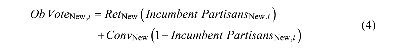
In this section, we present a formal argument regarding the normal vote and the personal vote. We begin with a simple model that characterizes the personal vote as something an incumbent gains independent of and on top of the normal vote. This is shown in Equation 1.

O b V o t e_{i} = N o r m a l V o t e_{i} + P e r s o n a l V o t e_{i}

where $O b V o t e_{i}$ is the proportion of the vote received by incumbent i in an election, $N o r m a l V o t e_{i}$ is the portion of the vote an incumbent receives from the electorate due to shared partisanship, and $P e r s o n a l V o t e_{i}$ is the proportion of the vote share received by the incumbent due to support from voters not normally inclined to support the incumbent due to partisanship, but do so because of the incumbent’s personal performance.

The term $N o r m a l V o t e_{i}$ in Equation 1 really consists of two components: the portion of the electorate that is normally inclined to support the incumbent based on partisanship, and the proportion of that group that actually does so. That second feature is absent in most cases because it is assumed to equal 1.

The term $P e r s o n a l V o t e_{i}$ in Equation 1 also consists of two components: the proportion of the electorate that is not normally inclined to support the incumbent based on partisanship and the proportion of that group that does so anyway. That proportion is generally assumed to be positive, but something less than 1.

The confusion in the literature stems from failing to unpack the normal vote and the personal vote into their two component parts. We label the proportion of the electorate inclined to support the incumbent based on party as Incumbent Partisans and the remainder as the proportion of the electorate not inclined to support the incumbent based on party. We include the rate parameters that are implicit, but hidden, in Equation 1. This allows us to rewrite the model as follows:

\begin{array}{l} O b s e r v e d V o t e_{i} = R e t (I n c u m b e n t P a r t i s a n s_{i}) + \\ C o n v (1 - I n c u m b e n t P a r t i s a n s_{i}) \end{array}

In Equation 2, Ret is short for “Retention,” and is a rate parameter that represents the actual proportion of the electorate normally inclined to support the incumbent due to partisanship that does so. Conv is short for “Conversion,” and is a rate parameter that represents the actual proportion of the electorate not normally inclined to support the incumbent due to partisanship that does so. Shifting attention to these rate parameters allows us to redefine both the normal vote and the personal vote in terms of performance.

Legislators certainly engage in casework, constituency service, and pork-barrel politics, but both constituents who share their legislator’s party affiliation and those who do not can benefit from these activities. Legislators also take positions on policies by introducing legislation, casting votes, and speaking on the floor. Some of the policy positions may be popular with voters from both parties, thereby enhancing their overall support, but other policy positions may appeal only to supporters of one party or the other. Legislators may perform poorly in office not only by failing to provide the particularized benefits associated with casework, constituency service, and pork-barrel politics, but also by adopting policy positions that are unpopular with voters of one or both parties. Finally, some legislators experience scandals that reduce their electoral support across the board.

We contend that how a legislator performs in office and how this performance translates into electoral support defines that legislator’s personal vote. In other words, the personal vote is really captured by a legislator’s performance and will reveal itself in the rate at which she retains the support of her partisans Ret and/or the rate at which she converts voters who would normally vote for candidates from the other party Conv. Our model leaves it as an empirical question, one that would focus on the degree to which these rate parameters are responsive to any electoral pressures or resources and whether those responses are negatively correlated (indicating a trade-off), positively correlated (indicating that they are complimentary), or not correlated (indicating that they are independent of each other). We turn next to identifying a feature that leads to clear predictions regarding how these rate parameters might respond.

Legislative Professionalism and the Personal Vote

The institutional arrangements of state legislatures affect both the incentive of incumbents to vigorously pursue reelection as well as their capacity to do so (e.g., Berry, Berkman, and Schneiderman 2000; Hibbing 1999; Squire 1997). Legislatures that offer more attractive seats should stimulate an incumbent’s interest in pursuing reelection relative to those legislatures with less attractive seats. Similarly, some legislatures provide incumbents with more resources they can use to pursue reelection. Because of its centrality to both the value of a legislative seat and the capacity of an incumbent to gain reelection, the institutional measure we focus on is legislative professionalism.

Berry, Berkman, and Schneiderman (2000) provide an extensive review of the concept of legislative professionalism (see also Squire and Hamm 2005). A more professionalized legislature enhances the attractiveness of a seat. It also provides resources that permit incumbents to insulate themselves from electoral pressures outside of their districts (Berry, Berkman, and Schneiderman 2000; Squire 1997). A dominant theme in the Congressional incumbency advantage literature is that expanding resources associated with professionalizing a legislature enhances an incumbent’s capacity to provide constituency service and casework, thereby building a personal vote (Cain, Ferejohn, and Fiorina 1987; Fiorina 1977; Jacobson 1990). Berry, Berkman, and Schneiderman (2000) assert that the insulating effect of professionalism may stem from legislators in more professional legislatures being able to provide both higher levels of constituency service and more effective governance compared with legislators operating in less professionalized legislatures.

If legislative professionalism affects legislative performance by affecting legislators’ motivation and capacity for pursuing reelection, then legislative professionalism should affect the personal vote received by a legislator, with higher levels of professionalism leading to a higher personal vote. Our definition of the personal vote implies that higher levels of professionalism may affect a legislator’s retention rate among her partisans, conversion rate among nonpartisans, or both.

Redistricting as a Natural Experiment

Following Ansolabehere, Snyder, and Stewart (2000) and Desposato and Petrocik (2003), we take advantage of the quasi-natural experiment presented by redistricting. The argument for a personal vote rests on the assumption that legislators establish relationships and reputations with their constituents as a result of their performance in office. When legislative districts are redrawn, many legislators end up with a sizable portion of their new district comprised of voters with whom the legislator does not have a history. The ability of a legislator to secure a performance-based personal vote from residents in the new portion of her district should be diminished relative to her capacity to cultivate a personal vote among residents in the old portion of her district.

Ansolabehere, Snyder, and Stewart (2000) analyze U.S House districts across several years while Desposato and Petrocik (2003) examine two election cycles in California for Congress and the State Assembly. In both articles, the authors compare those portions of districts that are new following redistricting to those old portions of the district. Ansolabehere, Snyder, and Stewart (2000) employ county-level election results for those districts consisting of more than one county, and for a subset of districts for which they have data at the township level, while Desposato and Petrocik (2003) use census block data matched to precinct-level election results. Both articles express the vote share received in each place (county, township, or precinct) by the Democratic candidate as a function of the normal vote in that place, whether the place is new or old to the district, and an interaction term between these two variables.⁶

Unfortunately, we do not have comparable data for state legislative elections. We can identify what portion of each district is old and new by comparing pre- and post-redistricting maps. We can measure the normal vote for both the old and new portions of the district by aggregating precinct-level election returns from the 2000 Presidential election. However, we cannot measure the vote share received by a state legislative candidate separately for both the old and new portions of the district. Rather, we can only observe the vote share received by a candidate for the entire district. However, unlike Ansolabehere, Snyder, and Stewart (2000) and Desposato and Petrocik (2003), we have data from multiple legislative elections conducted across multiple legislative institutional contexts, thus permitting the analysis of the impact of legislative professionalism on the retention and conversion parameters that define the personal vote. For these reasons, our empirical approach differs from those of Ansolabehere, Snyder, and Stewart (2000) and Desposato and Petrocik (2003).

A Model of Legislative Elections Following Redistricting

Recall that Equation 2 expresses the observed vote share received by a candidate as the sum of the portion the electorate normally inclined to support the incumbent based on partisanship that the incumbent retains and the proportion of the electorate not normally inclined to support the incumbent based on partisanship that is converted. We can break this down further after a redistricting by dividing a legislator’s district into its new and old portions:

\begin{matrix} O b V o t e_{Old, i} = R e t_{Old} (I n c u m b e n t P a r t i s a n s_{Old, i}) \\ + C o n v_{Old} (1 - I n c u m b e n t P a r t i s a n s_{Old, i}) \end{matrix}

\begin{array}{l} \begin{matrix} O b V o t e_{New, i} = R e t_{New} (I n c u m b e n t P a r t i s a n s_{New, i}) \\ + C o n v_{New} (1 - I n c u m b e n t P a r t i s a n s_{New, i}) \end{matrix} \end{array}

Equations 3 and 4 split the legislator’s district into its old and new portions, respectively. Next, the total observed vote can be written as the weighted average of the observed vote proportions from the old and new portions of the legislator’s district:

O b V o t e_{i} = P r o p_{O l d, i} (O b V o t e_{O l d, i}) + (1 - P r o p_{O l d, i}) (O b V o t e_{N e w, i})

If we substitute Equations 3 and 4 into Equation 5, we get the following result:

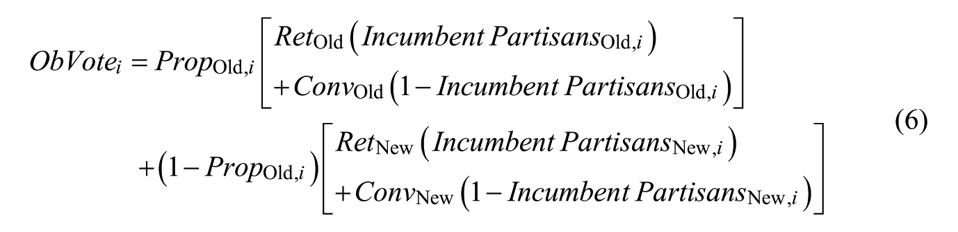
\begin{matrix} O b V o t e_{i} = P r o p_{Old, i} [\begin{array}{l} R e t_{Old} (I n c u m b e n t P a r t i s a n s_{Old, i}) \\ + C o n v_{Old} (1 - I n c u m b e n t P a r t i s a n s_{Old, i}) \end{array}] \\ + (1 - P r o p_{Old, i}) [\begin{array}{l} R e t_{New} (I n c u m b e n t P a r t i s a n s_{New, i}) \\ + C o n v_{New} (1 - I n c u m b e n t P a r t i s a n s_{New, i}) \end{array}] \end{matrix}

If the normal vote in the old and new portions of the district can be measured along with the proportion of a district that is new, we can estimate the four rate parameters in Equation 6. This can be seen more easily by multiplying out the terms in Equation 6 and rearranging them, like so:

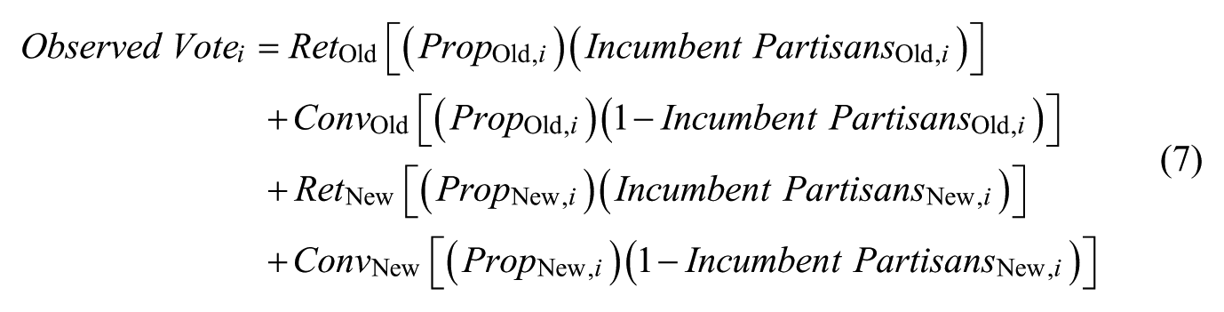
\begin{matrix} O b s e r v e d V o t e_{i} = R e t_{Old} [(P r o p_{Old, i}) (I n c u m b e n t P a r t i s a n s_{Old, i})] \\ + C o n v_{Old} [(P r o p_{Old, i}) (1 - I n c u m b e n t P a r t i s a n s_{Old, i})] \\ + R e t_{New} [(P r o p_{New, i}) (I n c u m b e n t P a r t i s a n s_{New, i})] \\ + C o n v_{New} [(P r o p_{New, i}) (1 - I n c u m b e n t P a r t i s a n s_{New, i})] \end{matrix}

Equation 7 shows that there are two retention parameters that could be estimated, one for the old portion of an incumbent’s district and one for the new portion of an incumbent’s district. The model also shows two conversion rate parameters to be estimated for the old and new portions of the incumbent’s district, respectively. Our conception of the personal vote focuses on generating estimates of these four rate parameters, making comparisons between them, and exploring how they respond to differences in legislative professionalism.⁷

As noted above and in Ansolabehere, Snyder, and Stewart (2000), most treatments of the normal vote assume that the normal vote translates into support for an incumbent on a one-for-one basis. This is equivalent to assuming that $R e t_{Old}$ and $R e t_{New}$ would be equal to 1. Similarly, a strict traditional interpretation of the personal vote would predict that $C o n v_{Old}$ would be positive but that $C o n v_{New}$ would be zero. This would indicate that an incumbent had cultivated some degree of support independent of shared partisanship in the old portion of her district but had not been able to do so yet in the new portion of her district. Thus, under traditional approaches to examining the personal vote, the only remaining empirical question would be to estimate the magnitude of $C o n v_{Old}$ .⁸ However, our discussion above makes clear that these are potentially unwarranted restrictions. Our reformulation of the concept of the personal vote requires estimating all four rate parameters in Equation 7.⁹ We then explore the impact of legislative professionalism on the personal vote by expanding the model in Equation 7 to allow each rate parameter to vary as a function of legislative professionalism.

Data and Method

Our primary source of data is ICPSR’s State Legislative Returns, 1967–2003 (Carsey et al. 2007) as described in Carsey et al. (2008) (ICPSR Study Number 21480). This data set includes basic information on all candidates running in general elections for state legislature, and allows for tracking candidates across successive elections—something essential for our analysis.

We limit our analysis to elections held in 2002 following redistricting due to the availability of GIS-compatible district maps and precinct-level presidential election returns. To simplify our analysis, we restrict our sample to incumbents running in single-member districts in either the upper or lower chamber of their legislature. We exclude cases where the incumbent ran unopposed, and include only Democratic and Republican incumbents. Some additional observations are lost due to missing data, leaving us with a sample of 1,610 observations spread across 41 states.

The dependent variable is the percentage of the vote received by the incumbent. Within our sample, this variable ranges between 10% and 100%, with a mean of 62.4 and a standard deviation of 10.3. To estimate the model in Equation 7, we also need to measure the proportion of each legislative district that is old as well as the share of the electorate in both the new and old portions of the district inclined to support the incumbent based on partisanship. Both tasks are accomplished using GIS software.¹⁰

Following a long list of previous scholars (see Ansolabehere, Snyder, and Stewart 2000), we measure the share of the electorate inclined to support the incumbent based on partisanship as the percentage of the two-party vote for President in 2000 cast for the presidential candidate of the incumbent legislator’s party. Ansolabehere, Snyder, and Stewart (2000) provide an extensive justification for using the presidential vote. In our case, the presidential vote in 2000 is also the only measure of the underlying partisan distribution of voters available to us. Many states do not require voters to register with a political party, and no other election results are systematically reported at the state legislative district level or at some smaller unit of analysis that we could aggregate to the level of the old and new portions of a state legislator’s district. However, 2000 presidential election vote shares are reported electronically at the precinct level and can be aggregated up to the old and new portions of a state legislative district using GIS. Fortunately, the 2000 Presidential election was a closely fought contest offering voters a choice between two candidates who were clearly separated from each other by partisanship. The result is that the observed vote distribution for the 2000 Presidential election should serve as a good proxy for the underlying distribution of partisanship more generally. More information on the construction of the data is provided in the appendix.

In our sample, the percentage of the post-redistricting district made up of voters from the legislator’s old district ranges from 4.3% to 100%, with a mean of 70.4 and a standard deviation of 22.8. The share of the electorate that voted for the Presidential candidate who shared the same party of the incumbent legislator for the old portion of a legislator’s district ranges from 13.7% to 98.3% with a mean of 57.3% and a standard deviation of 13.7. The same measure in the new portion of a legislator’s district ranges from 0% to 97.9%, with a mean of 50.1% and a standard deviation of 20.9. These two measures of the partisan make-up for the old and new portions of a legislator’s district are positively correlated (r = .47).¹¹

Finally, while several measures of legislative professionalism exist (Squire and Hamm 2005), we follow a number of scholars (e.g., Berry, Berkman, and Schneiderman 2000; King 1991; Van Dunk and Weber 1997; Weber, Tucker, and Brace 1991) by using the operating budget per member for a legislature.¹² For convenience of interpretation, we employ a linear transformation to scale the variable from zero to one, with zero indicating the lowest level of professionalism in the sample. The transformation is applied to all 50 states even though we only have observations from 41 states. Thus, while the theoretical range of the variable is from 0 to 1, the observed range of the variable in our data set is from .01 to .88. The mean of professionalism in our sample is .17, with a standard deviation of .16. Clearly, the professionalism measure has some extreme cases. In fact, its value falls below .4 for every state in our sample except for California. As a check, we reran our analyses dropping observations from California, and our results are virtually unchanged.¹³

Our discussion leads to several testable hypotheses. The traditional conception of the normal vote asserts that legislators should receive strong support of voters who share their party identification. The strictest interpretation of this view assumes that legislators would retain the full support of their partisans in both the old and new portions of their district following redistricting. This results in the prediction that $R e t_{Old}$ and $R e t_{New}$ would both equal 1. A weaker version of this proposition would allow for the defection of some partisans from an incumbent’s reelection coalition. Thus, $R e t_{Old}$ and $R e t_{New}$ may be less than 1, but if those defections remain strictly due to partisanship, $R e t_{Old}$ and $R e t_{New}$ should be equal to each other. Working from our definition, if the personal vote results in part from how legislators’ performances are evaluated by partisans in the old portion of their districts, and if their performances are evaluated as more positive than negative on average, then legislators should retain a higher proportion of their partisans in the old portions compared with the new portions of their districts. This is equivalent to predicting that $R e t_{Old}$ should be larger than $R e t_{New}$ . Each of these propositions can be expressed as a formal hypothesis:

Hypothesis 1 (H1): (Strong Traditional Normal Vote Hypothesis): $R e t_{Old}$ and $R e t_{New}$ should both be equal to one.

Hypothesis 2 (H2): (Weak Traditional Normal Vote Hypothesis): $R e t_{Old}$ and $R e t_{New}$ should be equal to each other.

Hypothesis 3 (H3): (Personal Vote Partisan Retention Hypothesis): $R e t_{Old}$ should be larger than $R e t_{New}$ .

Our discussion also generates hypotheses regarding the conversion rate of voters who do not share the party affiliation of the incumbent legislator. The traditional conception of the personal vote asserts that legislators generate support from those who do not share their partisan affiliation among voters who have experienced the service and performance of that legislator. The strongest version of this proposition predicts that a legislator will not receive any support in the new portion of her district from voters not from her party, but that she will receive some measurable support in the old portion of her district from voters not of her party. This is equivalent to predicting that $C o n v_{Old}$ will be positive while $C o n v_{New}$ will equal zero. A weaker version of this hypothesis would allow for some conversion among voters not of the legislator’s party in both portions of her district, but that the legislator should generate a higher conversion rate in the old portion of her district than in the new portion. Thus, this proposition predicts that $C o n v_{Old}$ will be larger than $C o n v_{New}$ .¹⁴ These propositions lead to the following specific hypotheses:

Hypothesis 4 (H4): (Strong Traditional Personal Vote Hypothesis): $C o n v_{Old}$ should be greater than zero while $C o n v_{New}$ should equal zero.

Hypothesis 5 (H5): (Weak Traditional Personal Vote Hypothesis): $C o n v_{Old}$ should be greater than $C o n v_{New}$ .

Following Berry, Berkman, and Schneiderman (2000) and the vast literature on the incumbency advantage in the U.S. Congress noted above, we expect that incumbents working in more professional state legislatures have a stronger incentive and a greater opportunity to cultivate a personal vote. Because the personal vote requires time and experience with a particular legislator, we expect this to be concentrated in the old portion of a legislator’s district. The traditional conception of the personal vote would predict that higher levels of legislative professionalism should be associated with an increase in $C o n v_{Old}$ . Our conception of the personal vote would not reject this prediction but would also predict that higher levels of legislative professionalism may improve a legislator’s retention rate among her own partisans in the old portion of her district. Thus, higher levels of legislative professionalism may be associated with an increase in $R e t_{Old}$ .

If legislative professionalism does permit a legislator to develop a stronger personal vote among voters in the old portion of her district, professionalism may also create a spillover effect in the new portions of her district. New voters in a legislative district may begin to learn more about the performance of their new legislator in the short time between redistricting and the first election that follows. Legislators in more professional legislatures may already be more visible to these voters, and they have more resources at their disposal to begin the process of developing a personal vote among their relatively new constituents. This potential spillover effect leads to the prediction that $R e t_{New}$ and/or $C o n v_{New}$ may also increase as the level of professionalism increases. These propositions can be stated as formal hypotheses:

Hypothesis 6 (H6): (Traditional Personal Vote and Professionalism Hypothesis): $C o n v_{Old}$ should increase as the level of professionalism increases.

Hypothesis 7 (H7): (Personal Vote Partisan Retention and Professionalism Hypothesis): $R e t_{Old}$ should increase as the level of professionalism increases.

Hypothesis 8 (H8): (Professionalism Spillover Hypothesis): Each of $R e t_{New}$ and $C o n v_{New}$ should increase as the level of professionalism increases.

We test H6, H7, and H8 by including four additional variables in the model presented in Equation 7. Each additional variable is computed by multiplying each component of the model by the level of professionalism in a state legislature.¹⁵

H1 through H8 emerge both from the existing literature on the normal vote and the personal vote as well as from our reconceptualization of the personal vote. These hypotheses do not exhaust the possible combinations of empirical findings that could emerge. Note also that several of these hypotheses are in conflict with each other. For example, H1 and H2 can both be supported simultaneously, but neither H1 nor H2 can be supported if H3 is supported. Our objective in this article is not to set up and support as many hypotheses as possible but rather to explore several basic hypotheses consistent with different conceptions of the normal vote and the personal vote in an effort to better understand how these concepts relate to each other.

Findings

We estimate the model presented in Equation 7 using OLS. The results are shown in column 1 of Table 1. Before turning to our specific hypotheses, we note that the results clearly show that incumbents enjoy a much higher rate of support from those who normally support candidates from their party compared with those who do not. Both retention rate parameters are estimated to be above .8, while both conversion parameters are estimated to be below .4—differences that easily attain traditional levels of statistical significance.¹⁶ We did not offer this as a formal hypothesis, but any theory of voting based on partisanship would predict this result.

Table 1.

Results from Ordinary Least Squares Models Estimating Retention and Conversion Rates in New and Old Portions of the Districts of Incumbent State Legislators Running for Reelection in 2002, with Robust Clustered Standard Errors in Parentheses.

Independent variables	Column 1	Column 2
Independent variables	Est. rate parameters	Est. rate parameters
$I n c . P a r t i s a n s_{Old} \times P r o p_{Old}$	.830 (.023)**	.773 (.025)**
$I n c . P a r t i s a n s_{New} \times (1 - P r o p_{Old})$	.859 (.047)**	.774 (.072)**
$(100 - I n c . P a r t i s a n s_{Old} \times P r o p_{Old})$	.384 (.035)**	.455 (.034)**
$(100 - I n c . P a r t i s a n s_{New} \times (1 - P r o p_{Old})$	.250 (.050)**	.337 (.081)**
$I n c . P a r t i s a n s_{Old} \times P r o p_{Old} \times P r o f$	—	.234 (.099)*
$I n c . P a r t i s a n s_{New} \times (1 - P r o p_{Old}) \times P r o f$	—	.546 (.267)*
$(100 - I n c . P a r t i s a n s_{Old} \times P r o p_{Old} \times P r o f)$	—	−.312 (.201)
$(100 - I n c . P a r t i s a n s_{New} \times (1 - P r o p_{Old}) \times P r o f)$	—	−.581 (.306)
R ²	.984	.985
N	1,610	1,610

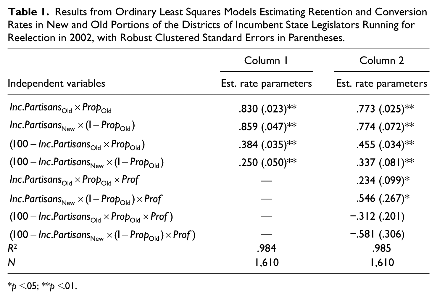
p ≤.05; **p ≤.01.

Turning to our specific hypotheses, H1 asserts that $R e t_{Old}$ and $R e t_{New}$ should both equal 1. We test this by comparing the model estimated in column 1 of Table 1 to a restricted model that constrains either $R e t_{Old}$ or $R e t_{New}$ to be equal to 1 using a standard F test. In this case, a statistically significant F test would indicate that $R e t_{Old}$ and $R e t_{New}$ , respectively, are statistically significantly different from 1. The test results for both $R e t_{Old}$ , F(1,40) = 56.68, p < .01, and $R e t_{New}$ , F(1,40) = 9.06, p $<$ .01, indicate that both retention rate parameters are significantly less than one. Thus, our findings lead us to reject H1. While the assumption that legislators retain the full support of their partisans is commonplace in the literature on the normal and personal vote, we do not find evidence to support that assumption in our analysis. Both in the old portions and the new portions of their districts, incumbent state legislators experience a statistically significant amount of slippage in their retention of party supporters.

The weaker version of the traditional normal vote hypothesis, H2, predicts only that the retention rate of partisans will be the same for legislators in the old and new portions of their districts. Given the results presented in column 1 of Table 1, this amounts to a test of whether the retention rate for the normal vote in the old portion of the district, estimated to be .83, differs significantly from the retention rate for the normal vote in the new portion of the district, estimated to be .86. This can be tested using a simple F test that compares the results of the model reported in Table 1 with a constrained model that forces $R e t_{Old}$ and $R e t_{New}$ to be equal to each other. The result of that test fails to reject the null of equality of these two retention rates, thus providing support for H2. Among incumbent state legislators, the retention rate of partisan supporters is not significantly higher or lower in the old portion of their districts compared with the new portion of their districts.¹⁷

By construction, finding support for H2 necessarily leads us to reject H3—that $R e t_{Old}$ would be greater than $R e t_{New}$ . One conclusion consistent with this finding is that the personal vote—support a legislator receives based on her performance in office—is not realized among partisans who have experience with the legislator compared with partisans newly added to her district. However, another possible conclusion is that the performance evaluation of legislators by partisans rests primarily on partisan matters rather than on nonpartisan casework or pork-barrel projects, making those performance evaluations easily absorbed by new partisans added to a legislator’s district.

H4, based on a strong traditional conception of the personal vote, predicted that the conversion rate among voters from the opposition party in the old portion of the district, $C o n v_{Old}$ , would be positive and significant, but that the conversion rate among voters from the opposition party in the new portion of the district, $C o n v_{New}$ , would equal zero. H4 can be tested using simple t-tests on the two estimated conversion rate parameters. Results presented in column 1 of Table 1 report that $C o n v_{Old}$ is estimated to be .38, which is statistically significant (t = 11.08, p $<$ .01). However, $C o n v_{New}$ is estimated to be .25 and also statistically significant (t = 4.95, p $<$ .01). Legislators clearly enjoyed a statistically significant positive level of support among those who do not share their partisan leanings in the old portion of their district, as H4 predicted, but they also enjoyed significant support among those who normally support the opposition party in the new portion of their district as well, in contradiction to H4.

The weaker version of the traditional personal vote hypothesis, H5, merely predicts that the conversion rate among nonsupporters of the incumbent’s party will be larger in the old portion of the incumbent’s district compared with the new portion. Testing H5 amounts to testing whether the estimate for $C o n v_{Old}$ of .38 is significantly larger than the estimated value for $C o n v_{New}$ of .25. The F test of this difference between the two conversion rates is statistically significant.¹⁸ Thus, we find clear evidence that incumbent state legislators generate a higher conversion rate among voters not inclined to support them due to partisanship within the old portion of their districts compared with the new portion of their districts. Unlike the retention rate of partisans, the conversion rate of nonsupporters of the incumbent’s party does appear to emerge more strongly among voters with a longer experience with the incumbent as their legislator.

To this point, we have uncovered evidence of a consistent and substantial normal vote in state legislative elections tied to partisanship. There is some slippage in the retention rate of partisans in these races, but that slippage is essentially equal across the old and new portions of a legislator’s district. Thus, we do not find evidence at this point that a personal experience with a legislator affects the retention rate among partisan supporters. However, we have documented a clear personal vote enjoyed by incumbent state legislators in the old relative to the new portion of their district in terms of their ability to convert voters who would normally support candidates of the opposition party. We attribute this to the personal experience these voters have with that incumbent. However, we also see that incumbent state legislators enjoy some degree of support even in the new portion of their districts among those not inclined to support them due to partisan leanings. This suggests that either incumbents are able to begin cultivating a personal vote in the new portion of their district prior to the first election following redistricting or that additional advantages beyond the personal vote accrue to incumbent state legislators seeking reelection.

Next, we turn to our results regarding the impact of legislative professionalism, presented in column 2 of Table 1.¹⁹ First, we note that the inclusion of the four interaction terms as a group significantly improves the overall fit of the model, F(4,40) = 3.31 (p $<$ .05). Because the specific coefficients operating on individual interaction terms and their statistical significance only tell part of the story regarding the conditional effect of professionalism, we turn to the estimated marginal effect of each component in our baseline model and how that effect varies across levels of professionalism. For example, the retention rate of partisans in the old portions of incumbents’ districts when the level of legislative professionalism is set at zero is .77 (the rate parameter displayed at the top of column 2 in Table 1). When legislative professionalism is increased to .2, this retention rate increases to .77 + (.23 × .2) = .82. Similar calculations can be performed for any level of legislative professionalism for all four of the rate parameters.

Rather than presenting a multitude of such calculations, we present the estimated level of each rate parameter across the observed range of legislative professionalism graphically in Figures 2 through 5. Each of these figures reports the level of legislative professionalism on the X-axis and the marginal effect of a given rate parameter on the Y-axis. The marginal effect is plotted as a solid line with dashed lines indicating a 95% confidence interval. A rug plot at the bottom of each figure illustrates the values of legislative professionalism as they appear in the data, with a slight random jitter added so that observations with identical values are not plotted on top of each other. Finally, because of the significant gap in values of legislative professionalism between California and all of the other states, we limit the range of professionalism in each plot to between 0 and .4.²⁰

Figure 2.

Estimated marginal effect of legislative professionalism on the retention rate in the old portion of a legislator’s district.

Figure 3.

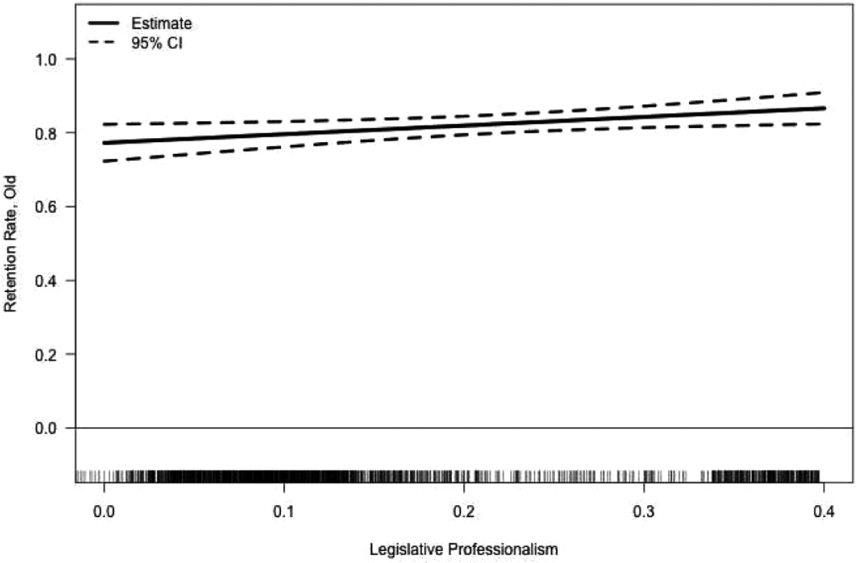
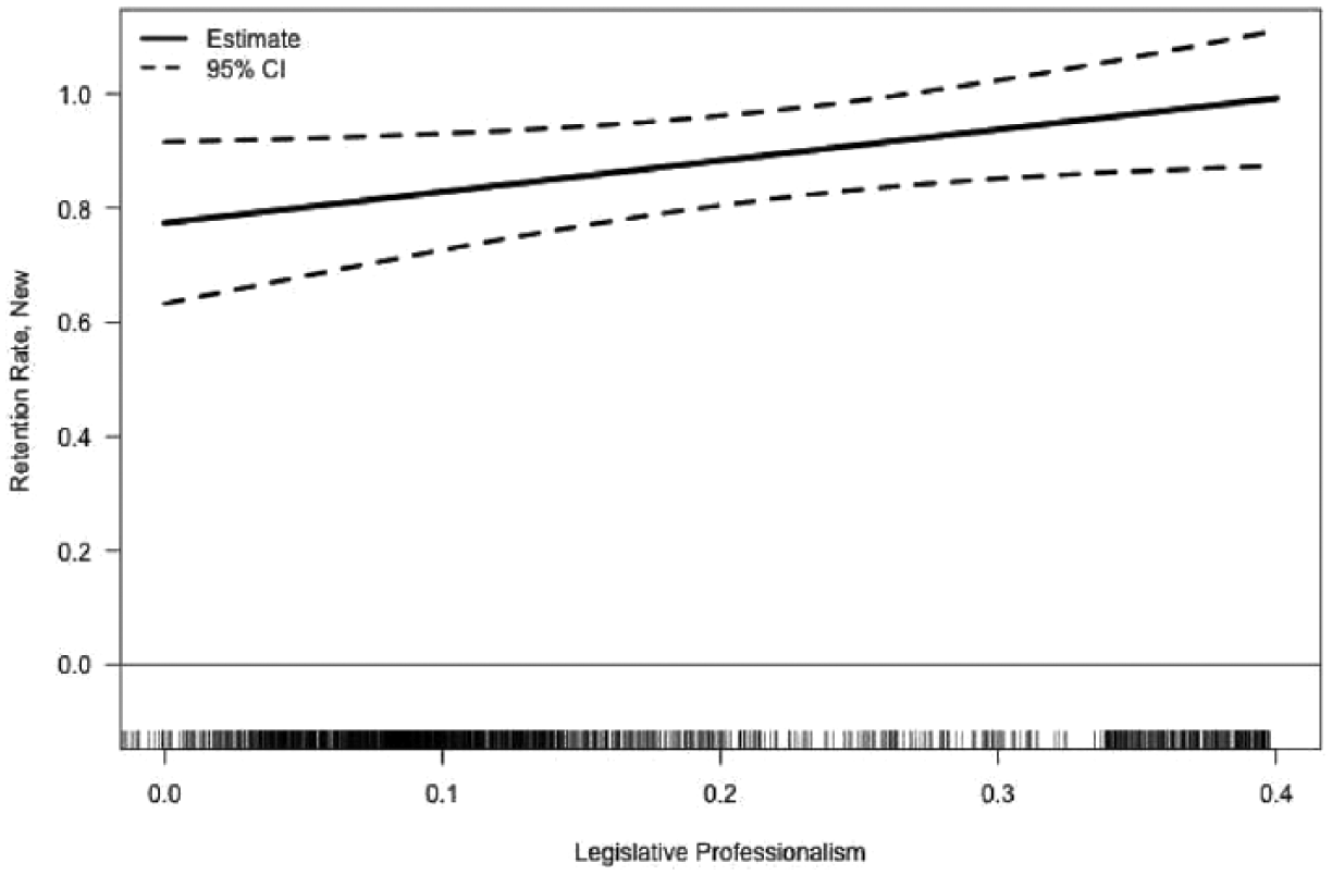
Estimated marginal effect of legislative professionalism on the retention rate in the new portion of a legislator’s district.

Figure 4.

Estimated marginal effect of legislative professionalism on the conversion rate in the old portion of a legislator’s district.

Figure 5.

Estimated marginal effect of legislative professionalism on the conversion rate in the new portion of a legislator’s district.

Figure 2 plots the estimated retention rate among partisans in the old portion of a legislator’s district as a function of the level of professionalism. At the lowest observed level of professionalism (professionalism = .01), the estimated retention rate of partisans by an incumbent in the old portion of her district is .77, with a 95% confidence interval ranging from .73 to .82. This retention rate increases significantly over the observed range of professionalism.²¹ In fact, our results show that the retention rate of partisans in the old portion of a legislator’s district becomes statistically indistinguishable from 1 when the level of professionalism reaches a value of about .6 on the 0 to 1 scale. The implication is that incumbents in highly professionalized legislatures can expect virtually full support of their partisans in the old portions of their districts. We interpret this finding as positive evidence that legislative professionalism facilitates the creation of a personal vote among an incumbent’s own partisans and, thus, supportive of H7.

Figure 3 presents similar results for the retention rate legislators receive in the new portions of their districts as a function of legislative professionalism. When professionalism is at its lowest observed value, this estimated retention rate is about .79, with a 95% confidence interval ranging from .64 to .92. This rate is comparable with the retention rate of partisans observed in the old portion of the district, but the wider confidence interval indicates greater variation in the retention rate among partisans in the new portion of legislators’ districts. We also find that a higher level of professionalism leads to a higher retention rate of partisans from the new portion of a legislator’s district. In fact, the rate of retention among partisans from the new portion of the district is statistically indistinguishable from 1 when legislative professionalism reaches a value of about .3 on the 0 to 1 scale, and the actual estimated retention rate itself reaches a value of 1 when legislative professionalism is at about .4. We think this result suggests a spillover effect of legislative professionalism among voters sharing the same party identification as the legislator, and thus, supportive of H8. In sum, increases in legislative professionalism appear to provide the average legislator with the ability to increase the rate at which she retains supporters from her own party among both those who have a history with her as their representative and those who do not. These increases are both statistically significant and substantively important.

Figure 4 presents our results for the conditional effect of legislative professionalism on the conversion rate legislators generate among voters who do not share their party leanings in the old portions of their districts. When professionalism is set at its lowest observed value, this estimated conversion rate is about .45 with a 95% confidence interval of .39 to .51. As legislative professionalism increases, however, this conversion rate actually declines. This decline is not statistically significant at tradition levels (as shown in column 2 of Table 1). The narrow and declining confidence intervals in Figure 4 at the lower range of legislative professionalism suggest a meaningful decline in $C o n v_{Old}$ as professionalism increases from its lowest value to values of about .2 (or about its observed mean). After that, the wider confidence intervals including a nearly flat upper bound give us greater uncertainty. However, across nearly the entire observed range of legislative professionalism, the conversion rate among nonsupporters of the legislator’s party remains statistically greater than zero. The conclusion we draw from Figure 4 is that if professionalism does have an impact on a legislator’s ability to convert supporters of the other party in the old portion of her district, that impact is negative. This runs counter to H6 and to the traditional notion that increased legislative professionalism would lead legislators to develop a stronger personal vote among those not already inclined to support them based on shared party affiliation.

Figure 5 presents our findings regarding the impact of legislative professionalism on the conversion rate an incumbent legislator enjoys among those who normally support candidates from the other party in the new portions of her district. At the lowest observed level of professionalism, this conversion rate is estimated to be .34 with a 95% confidence interval from .18 to .48. This estimated rate is lower than the conversion rate for the old portion of a legislator’s district. Also, the confidence interval around the conversion rate in the new portion of the district estimate is larger than it is for the conversion rate in the old portion of the district. However, Figure 5 shows the same weakly negative impact of legislative professionalism on the conversion rate of nonsupporters of the legislator’s party in the new part of the district that we found in the old part of the district. In fact, this conversion rate is statistically indistinguishable from zero when the value of legislative professionalism reaches about .38 on the 0 to 1 scale. Note that at all levels of legislative professionalism, the estimated conversion rate among nonsupporters of the legislator’s party is always higher in the old portion of the legislator’s district compared with the new portion. Wider confidence intervals associated with higher levels of legislative professionalism, however, mean that this difference in conversion rates is not statistically significant at levels of professionalism above about .42 on the 0 to 1 scale. Still, across most of our observed sample, legislators appear to enjoy a significant advantage among nonparty supporters in the old portions of their districts relative to nonparty supporters in the new portions of their districts.

Taken together, our findings suggest that the value of legislative professionalism to legislators seeking reelection comes from facilitating a higher retention rate among legislators’ partisans and not from the commonly held view that increased professionalism permits legislators to develop a stronger personal vote among constituents not already inclined to support the incumbent based on partisanship. While legislators appear to enjoy a significant personal vote among nonparty supporters in the old portion of their districts compared with the new portion of their districts, the overall rate at which legislators generate converts appears to hold steady at best, and may actually decline, as the level of legislative professionalism increases.

Conclusion and Discussion

In this article, we redefined the concept of the personal vote to focus on the rates at which legislators retain the support of their partisans and convert supporters of the opposition party. This changes the definition of the personal vote from being attached to a specific segment of the electorate to being based on the performance of incumbents and their ability to win support from all segments of the electorate. In turn, this shifts the notion of a trade-off between the personal vote and the normal vote as traditionally understood from an assumption to an empirical question.

We then presented an empirical model capable of estimating conversion and retention rates, taking advantage of legislative redistricting. We then examined how those rates are affected by the level of legislative professionalism in a state. We found that incumbent legislators do appear to enjoy a personal vote among voters who normally support candidates from the opposing party if those voters have a personal history of having been represented by that legislator. This finding is consistent with our reformulation of the personal vote as well as traditional understandings of it.

Contrary to traditional understandings, we found that increases in legislative professionalism enhanced a legislator’s personal vote through increasing the rate at which she retained supporters from her own party in the old portions of her districts, and that this effect appears to spill over to partisans in the new portion of her district as well. In contrast, legislative professionalism did not help incumbents increase the conversion rate among nonpartisans. In short, legislative professionalism may help incumbents insulate themselves electorally (e.g., Berry, Berkman, and Schneiderman 2000), but it appears to do so by enhancing their ability to retain their own partisans rather than developing greater support among those who normally support candidates of the other party. A history with the incumbent increases the conversion rate among nonpartisans, but professionalism increases the retention rate among partisans. These findings suggest that our redefinition of the personal vote may both alter and improve our understanding of the electoral connection between voters and legislators and how that connection is mediated by institutional characteristics.

Footnotes

Appendix

In constructing our dataset, we began with precinct level data in each state from the 2000 presidential election. The precinct data included the pre-redistricting legislative district and the presidential vote. We then mapped the year 2000 precincts into the year 2002 legislative districts. In most states, we accomplished this using GIS techniques. We collected what are called shape files for the states’ precincts and 2002 legislative districts. We then overlaid the new districts onto the precincts to determine the new district for each of the precincts. This is similar to the method used by Desposato and Petrocik (2003) in which they focused on Census block changes in California districts. In some states, GIS data were not available at either the 2002 district or precinct level. In these cases, we gathered a list of the precincts with their new district designations and then merged these lists into our initial precinct data. Both techniques provided the same result.

With this information, we were able to aggregate the precinct data into the appropriate district-level variables. We construct measures of district change by calculating the percentage of an incumbent’s district made up of new precincts (or voters) compared with the percentage of the district consisting of old precincts (or voters). We calculated the normal vote in both the old and new portions of an incumbent’s district by aggregating the share of the two-party vote for president received by the incumbent legislator’s party in those precincts that make up the old and new portions of the legislator’s district.

In constructing our data, a few problems emerged. In a few states, precincts are split into multiple districts. We are unable to determine the exact detail of these splits and cannot accurately trace the presidential vote at the sub-precinct level into the appropriate districts. In addition, a few states or counties redrew or reconfigured their precincts as part of their redistricting, which made it difficult to accurately identify the normal vote in new districts constructed using new precincts based on the presidential vote share recorded based on the old precincts. In most cases, states provided conversion sheets that allowed us to track these changes. In some areas with fast growing populations, states split existing precincts to compensate for the population growth. In most cases, the newly split precincts remained in the same legislative district and, therefore, did not cause us any problems. In a few cases, however, the newly split precincts were drawn into separate districts. In these cases, we could not accurately account for the presidential vote at the sub-precinct level.

Once we constructed these measures, we merged the variables with the district-level state legislative election returns (SLER) data using state, chamber, and district identifying information. The SLER data records the vote share received by every major party candidate and nearly all minor party candidates running for the state legislature from 1967 through 2003. For this article, we made use of the data for elections held in 2002 following a state’s legislative redistricting as well as data from the election that directly preceded redistricting. Using both the pre- and post-redistricting data allowed us to identify incumbents running in 2002. Critical to that process is ensuring that candidate names are recorded in exactly the same way for every year an individual candidate runs. For more detailed information about this data, see http://www.unc.edu/carsey/research/datasets/data.htm. For more information about the process of making sure that the name variable is properly recorded, see http://webapp.icpsr.umich.edu/cocoon/ICPSR-STUDY/03938.xml.

Acknowledgements

Carsey and Berry gratefully acknowledge the support for this research provided by the National Science Foundation (SES-0317924). Carsey thanks participants in a departmental colloquium at Brigham Young University for their comments and suggestions, as well as Jane Carsey for her assistance with the replication code.

Declaration of Conflicting Interests

The author(s) declared no potential conflicts of interest with respect to the research, authorship, and/or publication of this article.

Funding

The author(s) disclosed receipt of the following financial support for research, authorship, and/or publication of this article: This study was supported by the National Science Foundation (SES-0317924).

Notes

Author Biographies

Thomas M. Carsey is the Thomas J. Pearsall Distinguished Professor of political science at the University of North Carolina at Chapel Hill. Carsey has served as editor of State Politics and Policy Quarterly, President of the Southern Political Science Association, and Director of the Odum Institute for Research in Social Science at UNC. His research interests focus on representation in American politics and research methods.

Jonathan Winburn is an Associate Professor of political science and Director of the Social Science Research Lab at the University of Mississippi. His research focuses on representation, redistricting, elections, public policy, and state politics. He has served as webmaster for the State Politics and Policy section of the American Political Science Association since 2008.

William D. Berry is the Syde P. Deeb Eminent Scholar and Marian D. Irish Professor of political science at Florida State University, where he is also the Director of the Center for the Study of Democratic Performance. His research interests focus on public policy, state politics, and research methods.

References

Ansolabehere

Stephen D.

Jr. Snyder

James M.

Stewart

Charles

III . 2000. “Old Voters, New Voters, and the Personal Vote: Using Redistricting to Measure the Incumbency Advantage.” American Journal of Political Science 44 (1): 17–34.

Berry

William D.

Berkman

Michael B.

Schneiderman

Stuart

. 2000. “Legislative Professionalism and Incumbent Reelection: The Development of Institutional Boundaries.” American Political Science Review 94 (4): 859–74.

Brambor

Thomas

Clark

William Roberts

Golder

Matt

. 2006. “Understanding Interaction Models: Improving Empirical Analyses.” Political Analysis 14 (Winter): 63–82.

Cain

Bruce

Ferejohn

John

Fiorina

Morris P.

1987. The Personal Vote. Cambridge: Harvard University Press.

Campbell

Angus

Converse

Philip E.

Miller

Warren E.

Stokes

Donald E.

1960. The American Voter. New York: Wiley.

Carsey

Thomas M.

Berry

William D.

Niemi

Richard G.

Powell

Lynda W.

Snyder

James M.

2007. State Legislative Election Returns, 1967-2003. ICPSR 21480-v1. Ann Arbor: Inter-university Consortium for Political and Social Research. doi:10.3886/ICPSR21480.v1.

Carsey

Thomas M.

Niemi

Richard G.

Berry

William D.

Powell

Lynda W.

Snyder

James M.

Jr.

2008. “State Legislative Elections, 1967-2003: Announcing the Completion of a Cleaned and Updated Dataset.” State Politics & Policy Quarterly 8 (4): 430–43.

Converse

Philip E.

1966. “The Concept of the Normal Vote.” In Elections and the Public Order, edited by Campbell

Angus

9–39. New York: Wiley & Sons.

Desposato

Scott W.

Petrocik

John R.

2003. “The Variable Incumbency Advantage: New Voters, Redistricting, and the Personal Vote.” American Journal of Political Science 47 (1): 18–32.

10.

Downs

Anthony

. 1957. An Economic Theory of Democracy. New York: Harper & Row.

11.

Enelow

James M.

Hinich

Melvin J.

1984. The Spatial Theory of Voting: An Introduction. New York: Cambridge University Press.

12.

Fenno

Richard F.

1978. Home Style: House Members in Their Districts. Boston: Little, Brown.

13.

Fiorina

Morris P.

1977. Congress: Keystone of the Washington Establishment. New Haven: Yale University Press.

14.

Friedrich

Robert J.

1982. “In Defense of Multiplicative Terms in Multiple Regression Equations.” American Journal of Political Science 26:797–833.

15.

Hibbing

John R.

1999. “Legislative Careers: Why and How We Study Them.” Legislative Studies Quarterly 24:149–71.

16.

Jacobson

Gary C.

1990. The Electoral Origins of Divided Government: Competition in U.S. House Elections, 1946-1988. Boulder: Westview Press.

17.

Jacobson

Gary C.

2004. The Politics of Congressional Elections. 6th ed. New York: Pearson Longman.

18.

King

Gary

. 1991. “Constituency Service and the Incumbency Advantage.” British Journal of Political Science 21:119–28.

19.

Mayhew

David R.

1974. Congress: The Electoral Connection. New Haven: Yale University Press.

20.

Squire

Peverill

. 1997. “Another Look at Legislative Professionalism and Divided Government in the States.” Legislative Studies Quarterly 22:417–33.

21.

Squire

Peverill

Hamm

Keith E.

2005. 101 Chambers: Congress, State Legislatures, and the Future of Legislative Studies. Columbus: Ohio State University Press.

22.

Van Dunk

Emily

Weber

Ronald E.

1997. “Constituency-Level Competition in the U.S. States, 1968-1988: A Pooled Analysis.” Legislative Studies Quarterly 22:141–59.

23.

Weber

Ronald E.

Tucker

Harvey J.

Brace

Paul

. 1991. “Vanishing Marginals in State Legislative Elections.” Legislative Studies Quarterly 16:29–47.