Responding to Low Coefficient Alpha: Potential Alternatives to the File Drawer

Abstract

To the detriment of human resource development (HRD) theory building and research, many scholars may think that research data with a low coefficient alpha is destined for the file drawer; this does not have to be the case. Contemporary literature suggests that many scholars do not know how to move forward with data that yields α < .70. In addition, an investigation revealed that many scholars practice the method of item deletion to increase alpha. Besides supporting the case that discarding research simply because of low coefficient alphas may be unnecessary, a guide is presented to demonstrate how scholars and scholar–practitioners may be able to analyze data when an initial estimate of internal reliability is low. We caution that deleting items may increase reliability at the cost of validity. As an alternative, this study demonstrates that eliminating subjects can increase alpha and maintain the integrity of the scale. This guide presents generalizability theory as a means to identify the source of error variance in data as well as a step-by-step process to correct for low coefficient alpha. The guide is illustrated with data and R syntax.

Keywords

low coefficient alpha statistical reliability internal reliability

Social and behavioral science researchers require validated theory to undergird their research, which can subsequently be used to inform interventions. Thus, in a wide range of social and behavioral disciplines such as human resource development (HRD), psychology, education, economics, management, anthropology, and sociology (Chalofsky, 2007), theories are the tools researchers need to support hypothesis development and testing. Furthermore, it is the said theory undergirding a study that researchers then use to interpret and make sense of often disparate findings. The new knowledge reaped from the empirical findings consequently enrich what we already knew about the theory and its validity as a tenable theory to support new understandings of intrapersonal, interpersonal, team, group, and organizational phenomena. Undeniably, theory building and testing is an essential part of the scientific endeavor; without it, we would be limited to making “common sense” or “naïve” attributions about how and why things occur that can be untrue (Heider, 1958; Kelly, 1992), rather than using theoretically based, rigorous research to make valid conclusions about the antecedents and consequences of attitudes, beliefs, emotions, motivations, and behaviors.

Highlighting the importance of theory building and testing to the field of HRD, a recent issue of Advances in Developing Human Resources (21[3]) was dedicated to examining the theoretical foundations of HRD and its implications for HRD research (Bakeret al., 2019). In that issue, adaptive structuration, agency, feminist, employee engagement, social identity, and social presence theories were explored and touted as useful lenses through which to develop new HRD research and concomitantly interpret results based upon that research. In a similar but more technical journal issue, Nimon et al. (2015) co-edited an Advances in Developing Human Resources (17[1]) issue investigating quantitative data-analytic techniques and how and why they were important for HRD theory and practice. The Nimon et al. (2015) issue built upon the notion that quantitative methods were useful for theory building and testing, understanding that certain assumptions must be adhered to carefully to avoid introducing systematic error into the study and in a more distal sense, error into the extant literature that might lead to designing flawed future studies that would be detrimental to theory-building efforts in the field. In that issue, Song and Lim (2015), for example, discussed how mediation analysis was an appropriate statistical tool for enriching theory-building efforts, as it allows researchers to calculate the direct and indirect effects of independent and mediating variables on outcome variables. The new knowledge generated by the research designed with theoretically and practically relevant mediator variables in mind can be used subsequently to support future research studies and theory building.

Still, the results of quantitative analyses can be interpreted with confidence, as with any research, only if certain methodological and/or statistical assumptions have been met. One major assumption is that the scores derived from the research instruments are statistically reliable and valid. Understanding that there is no such thing as a perfect research measure (Schmidt & Hunter, 2014), researchers must be attentive especially to the reliability and validity related to the scores of the measurement tools employed in their respective studies. For the purposes of this research, we focus upon reliability, defined as a measure of the consistency or stability of scores on a measure (Thompson, 2003). We refer the reader to explore validity issues in Thompson and Daniel (1996) and Thompson (2004).

The Wilkinson et al. (1999) cautioned, “It is important to remember that a test is not reliable or unreliable,” reliability is a measure of test scores for the specific population of the current study (p. 596). For example, in the case of a population of 200, four samples could yield alphas that range from .59 to .84. We will illustrate below the effect that individual responses have on coefficient alpha, after presenting some preliminary background thoughts and a review on reliability as well.

Because it continues to be the most widely used reliability measure in the social and behavioral sciences (Cortina, 1993; Cronbach & Shavelson, 2004), we examine coefficient alpha. We are particularly interested in issues related to handling low alpha coefficients because they increase the likelihood of not being published in a peer-reviewed journal, which is unfortunate because there are ways to handle this situation that can preclude the perceived need for reviewers and editors to summarily reject such research. This state of affairs can be problematic since opportunities for theoretical enrichment in the field of HRD may be unnecessarily lost to the detriment of all.

Background of the Study

A recent review of the “Questions Forum” on Research Gate revealed 35 posts asking for guidance on how to continue research analysis when coefficient alpha is below .70. Coefficient alpha .70 is widely accepted as the benchmark for score reliability (Kaplan & Saccuzzo, 1982; Murphy & Davidshofer, 1988; Nunnally, 1978). As such, Bonett and Wright (2015) stated that they “have both heard numerous reports where manuscripts were rejected simply because the sample value of coefficient alpha was below 0.70” (p. 4). Also, Greco et al. (2018) reviewed 1,296 studies made up of 1,675 independent samples and found that alphas consistently exceeded .70 and by and large were above .80.

Intrigued by the discussion board comments, we considered the possibility that many researchers do not know how to proceed with data when alpha is low. Consequently, studies often end up in the proverbial file drawer (cf. Bosco, 2018). We agree with scholars (e.g., Thompson, 2003) that assessing internal reliability is essential to rigorous research. However, even if a reliability coefficient is low, the data or subsets of the data may still be useful for analysis that enriches empirical, conceptual, and theoretical understandings. For these reasons, we developed a guide to help scholars and scholar–practitioners process data that initially yield low estimates of reliability that can contribute meaningfully to theory building.

Classical Test Theory and Reliability

The concept of reliability was presented in 1904 when Spearman formulated ways to evaluate score reliability that are known today as classical test theory (Thompson, 2003). Classical test theory assumes that observed scores are comprised of true score and measurement error and that total score variance is comprised of observed score and measurement-error variance. Unlike other reliability theories, classical test theory does not consider systematic error in the estimation of measurement error.

In 1910 Spearman and Brown articulated the Spearman–Brown prophecy formula. The formula “provides a rough estimate of how much the reliability of test scores would increase or decrease if the number of observations or items in a measurement instrument were increased or decreased” (Brown, 2018, p. 1558). Commonly known as split-half reliability, a correlation coefficient for each half of the instrument, commonly the odd-numbered and even-numbered items, is calculated. The Spearman–Brown formula is applied to the estimate of the reliability of each half to calculate the full-test reliability (Brown, 2018). Scholars criticized the split-half technique, stating that “the two coefficients are measures of different qualities and should not be identified by the same unqualified appellation reliability” (Cronbach, 1951, p. 298).

In 1931, Kuder and Richardson, critics of the split-half technique, developed two algebraic equations (the Kuder–Richardson Formula 20 and the Kuder–Richardson Formula 21) to extract the coefficient of equivalence, an estimation of reliability, from one set of data (Cronbach, 1951). Thompson (2003) explained that “the seminal formula for an estimate of internal consistency can be traced to the famous algorithm presented as the 20th formula within the article by Kuder and Richardson (1937)” (p. 11). The Kuder–Richardson Formula 20 became the focus of Cronbach’s (1951) Psychometrika article that introduced coefficient alpha. The formulas are conceptually similar. However, the Kuder–Richardson Formula 20 works only for dichotomous item scores, while coefficient alpha can be computed from dichotomous and nondichotomous item scores (Thompson, 2003). Sixty-eight years later, Cronbach’s article has been cited 43,259 times (Google Scholar, February 11, 2020).

Coefficient Alpha

According to Cronbach (1951), coefficient alpha is the “mean of all possible split-half coefficients” (p. 331). From this perspective, Henson (2001) cautioned researchers to realize “that internal consistency coefficients are not direct measures of reliability, but rather are theoretical estimates derived from classical test theory” (p. 177). Cronbach stated that “alpha estimates the proportion of the test variance due to all common factors among items. That is, it reports how much the test score depends upon general and group rather than item specific factors” (p. 320). With that in mind, Gronlund and Linn (1990) explained that “reliability refers to the results obtained with an evaluation instrument and not to the instrument itself. Thus, it is more appropriate to speak of the reliability of ‘test scores’ or the ‘measurement’ than of the ‘test’ or the ‘instrument’” (p. 78). Indeed, the idea that tests are not reliable led Vacha-Haase (1998) to propose a measurement meta-analytic technique, reliability generalization and for Thompson and Vacha-Haase (2000) to recognize that “psychometrics is data metrics” (p. 174). As such, coefficient alpha is influenced by sample characteristics (sample size and heterogeneity or homogeneity), the number of test items, or interrelatedness between items (Multon & Coleman, 2010; Tavakol & Dennick, 2011). For these reasons, it is imperative to measure reliability for every study conducted rather than citing reliability estimates from previous research.

As noted by Henson (2001, pp. 180–182), coefficient alpha can be calculated with either equation 1 or 2, where k equals the number of items in the scale, $Σ σ_{k}^{2}$ equals the sum of all the k item variances, $σ_{TOTAL}^{2}$ equals the variance of the total scale scores, and $Σ COV (for i < j) \times 2) = the doubled sum of the unique covariances$ :

α = \frac{k}{(k - 1)} [1 - (\frac{Σ σ_{k}^{2}}{σ_{TOTAL}^{2}})],

(1)

α = \frac{k}{(k - 1)} [1 - (\frac{Σ σ_{k}^{2}}{(Σ σ_{k}^{2} + Σ {COV}_{i j} (for i < j) \times 2)})] .

(2)

If data are standardized, alpha is simply a function of the average interitem correlation (r) as shown in equation 3 (Helms et al., 2006, p. 640; Kopalle & Lehmann, 1997):

α = \frac{k r}{(1 + [k - 1] r)} .

(3)

The higher the value, the greater the reliability. Coefficient alpha of .70 means that 30% of the variance in the data is theoretically measurement error. Acceptable ranges for alpha vary among scholars. Nunnally (1967) stated that, in “the early stages of research on predictor tests or hypothesized measures of a construct, . . . reliabilities of .60 or .50 will suffice” (p. 226). He further recommended .80 for basic research and .90 for applied settings in which the cutoff score is important. In the second edition of his seminal work, Nunnally (1978) raised the benchmark for exploratory research to .70 (pp. 245–246). As noted by Henson (2001) and others, this led many researchers to reference Nunnally (1978) if they attained a coefficient alpha of .70 or higher and Nunnally (1967) if they attained a coefficent alpha of .60 or .50. Kaplan and Saccuzzo (1982) argued that .70 to .80 is an acceptable range for basic research, and for practical research, the level should be .95 (p. 106). With a seemingly more tolerant approach, Murphy and Davidshofer (1988) stated that below .60 is unacceptable, .70 is low, .80–.90 is moderate to high, and .90 is high. Multon and Coleman (2010) explained that the acceptable range should be based partly on the context of what is being measured. Although scientists continue to disagree on the acceptable level of coefficient alpha, the levels suggested by Murphy and Davidshofer (1988) and Nunnally (1978) are the most cited (Google Scholar, Feburary 11, 2020).

Coefficient alpha is ideal for HRD researchers due to its effective reliability assessment of traits such as job satisfaction, organizational justice, and workplace behaviors (Multon & Coleman, 2010). Two additional benefits worth noting are (a) that confidence intervals (CIs) can be constructed around alpha and (b) that coefficient alpha is robust to violations of underlying assumptions (Reinard, 2006).

Fan and Thompson (2001) urged authors to report CIs with score reliabilities along with the estimation method used to determine the values. CIs for coefficient alpha are calculated as indicated in equations 4 and 5, where $\hat{a}$ = sample coefficient alpha, $γ$ = significance level, F = F distribution for percentiles for γ/2 and 1 − γ/2, n represents the sample size, k = number of items, df1 = n − 1, df2 = (n − 1) (k − 1) (Thompson, 2003, p. 75):

{CI}_{lower} = 1 - [(1 - \hat{α}) F_{(1 - γ / 2), d f 1, d f 2}],

(4)

{CI}_{upper} = 1 - [(1 - \hat{α}) F_{γ / 2, d f 1, d f 2}] .

(5)

There are four assumptions to coefficient alpha: (a) the scale adheres to tau equivalence; (b) scale items are on a continuous scale and have the same or reasonably same distribution shapes; (c) the errors of the items do not covary; and (d) the scale is unidimensional (McNeish, 2018, p. 414). These assumptions are also limitations to coefficient alpha. As it relates to the first assumption, McNeish (2018) explained that “tau equivalence is the statistically precise way to state that each item on a scale contributes equally to the total scale score” (p. 415). To meet this assumption, the standardized factor loadings for every item would have to be practically analogous. For the second assumption, most software implementations of coefficient alpha (e.g., R, SAS, and SPSS) calculate item covariances using a Pearson covariance matrix. Pearson covariance matrices assume that the variables are continuous and normal. However, if data are binary, coefficient alpha will underestimate the level of reliability (McNeish, 2018). Third, coefficient alpha assumes that the item errors do not covary. There are a number of situations that may cause the errors to correlate, resulting in an over- or underestimation of alpha (e.g., the order of the items on the scale, transient responses, or unmodeled multidimensionality; McNeish, 2018). Finally, “unidimensionality is the degree to which the items all measure the same underlying construct” (Schmitt, 1996, p. 350). Schmitt (1996) pointed out that “internal consistency refers to the interrelatedness of a set of items, whereas homogeneity refers to the unidimensionality of the set of items” and the “confusion in the literature involves the use of homogeneity and internal consistency as though they were synonymous” (p. 350).

Generalizability Theory and Reliability

With major developments in mathematical statistics, Cronbach no longer considered “the alpha formula as the most appropriate way to examine most data” (Cronbach & Shavelson, 2004, p. 403). Based on his revelation, Cronbach began to sketch the components of variance approach to reliability from which he and his associates developed the generalizability theory (G theory; Cronbach et al., 1963, 1972).

Cronbach observed that

Measurement specialists have often spoken of a test as a sample of behavior, but the formal mathematical distinction between sample of persons and populations of persons, or between a sample of tasks and a population [a universe] of tasks, was rarely made in writings on test theory in 1951 and earlier. (Cronbach & Shavelson, 2004, p. 404).

Quantitative HRD research is not as interested in any one score; rather, it is interested in how that score can be applied to behavior in a broader context. Cronbach et al. (1972) called this the universe score. Shavelson et al. (1989) explained that “a score’s usefulness, then, largely depends on the extent to which it allows us to generalize accurately to behavior in some wider set of situations, a universe of generalization” (p. 922). G theory “recognizes that there may be multiple definitions of true- and error-scores.” Multiple sources of error define the universe of generalization, a fundamental notion in G theory that “a measurement taken on a person records a sample of behavior” (i.e., a score; Shavelson et al., 1989, p. 922). Cronbach et al. (1972) surmised that “the question of reliability thus resolves into a question of accuracy of generalization, or generalizability” (p. 15).

As previously mentioned, coefficient alpha provides an estimate of true score variance. For example, α = .70 suggests that the remaining 30% is measurement error. However, the source of the measurement error variance is unknown. On these grounds, when coefficient alpha is low, a G study can be performed to partition observed variance across effects (e.g., person, item, and the interaction between person and item, along with model specification error). The effects can be used to compute a generalizability coefficient that results in the same value as coefficient alpha (Webb et al., 2006).

Our discussion of G study reflects the parsimonious one-facet design where an observed score for a particular person on a particular item is decomposed into an effect for the grand mean, plus effects for the person, the item, and a residual including the interaction between person and item and unsystematic error (Webb & Shavelson, 2005). Since person is the object of measurement, it is not a source of error and as such, item is the only facet (i.e., one-facet design; Webb & Shavelson, 2005). In a one-facet design, observed variance is decomposed into three components, as shown in Table 1 (cf. Shavelson & Webb, 1981, p. 2).

Table 1.

Observed Score, Mean Variance, and Generalizability Coefficient Variance Components for p × i Design.

Observed score		Mean variance					Generalizability coefficient
Effect	Component	Effect	Score variance component	F	MVC	MVC percentage	Effect	MVC(s)
I	$μ_{i} - μ$	i	$σ_{i}^{2}$	K	$\frac{σ_{i}^{2}}{f}$	$\frac{{MVC}_{i}}{Σ MVC}$
p	$μ_{p} - μ$	p	$σ_{p}^{2}$	1	$\frac{σ_{p}^{2}}{f}$	$\frac{{MVC}_{p}}{Σ MVC}$	Systematic	${MVC}_{p}$
pi, e	$X_{p i} - μ_{p} - μ_{i} + μ$	pi, e	$σ_{p i, e}^{2}$	K	$\frac{σ_{p i, e}^{2}}{f}$		Measurement Error	${MVC}_{p i, e}$
Total	$X_{p i}$	Total			$Σ MVC$	$\frac{{MVC}_{p i, e}}{Σ MVC}$	Total	${MVC}_{p} + {MVC}_{p i, e}$

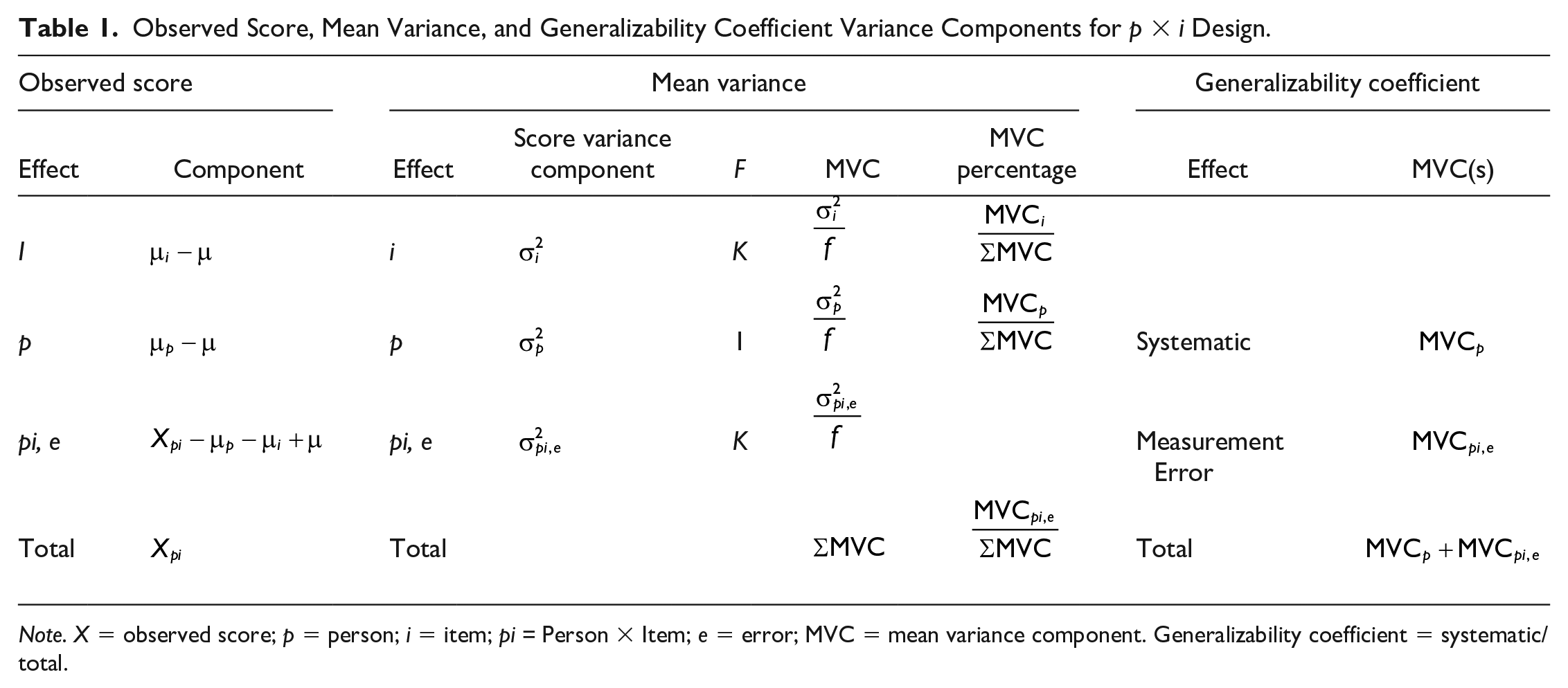
Note. X = observed score; p = person; i = item; pi = Person × Item; e = error; MVC = mean variance component. Generalizability coefficient = systematic/total.

The item effect (i) is the variance of constant errors related to the item; the person effect (p) is equivalent to the true-score variance of classical test theory; and the remaining effect pi, e represents the interaction between the person and item effects along with unidentified sources of measurement error (Shavelson & Webb, 1981). Usually, G theory presumes that all the ways of the measurement design are random effects (Thompson, 2003, p. 52). Therefore, the score variance components are typically derived using processes that model random effects (e.g., hierarchical linear modeling). Each mean variance component (MVC) is calculated by dividing the score variance component by the frequency of the effect. The MVC of each effect is divided by the total MVC to estimate the component percentage (see Table 1).

The component percentages in G theory can inform the researcher. Take, for example, dichotomously scored items such as those that can be evaluated as right or wrong. A large component percentage for i might suggest that the items varied in difficulty and were a source of unwanted measurement error. A large component percentage for p would suggest that the sample differed systematically in their feelings of the factors measured. A large component percentage for pi, e would suggest that the relative standings of persons varied across items. With that said, remember that the MVC for pi, e contains the interaction between person and item as well as unspecified measurement error variance which cannot be subpartitioned from the pi variance, due to degree of freedom restrictions (Shavelson et al., 1989).

When people are defined as the object of measurement, the person MVC constitutes systematic score variance, and all other MVCs are measurement error variances. As noted by Thompson (2003), “having variance from people being large is a desirable outcome if our premise in a given study is that people differ as individuals and that it is exactly these differences that we wish to quantify or study” (p. 54). In the one-facet design, the measurement error in the generalizability coefficient is the pi, e MVC. The generalizability coefficient is the systematic score variance divided by systematic score variance plus measurement error, as illustrated in Table 1.

Proposed Method for Processing Data With Low Coefficient Alpha

Data with low coefficient alpha should first be evaluated for missing data and outliers. Missing data can occur when a respondent does not provide an answer for one or more items on the scale. Missing data can be treated through a variety of techniques including listwise deletion, pairwise deletion, mean imputation, regression imputation, and maximum likelihood estimation (cf. Edwards & Finch, 2018). However, research suggests that the processing of missing data can have a deleterious impact on coefficient alpha (cf. Enders, 2004; Van Ginkel et al., 2007). For example, Enders (2004) found that the traditional method of listwise deletion yielded biased reliability estimates as compared with methods that incorporated maximum likelihood estimation techniques. Enders suggested that in addition to reporting CIs with reliability coefficients as suggested by Fan and Thompson (2001), missing data and how it was dealt with should also be reported. Edwards and Finch (2018) recommended that the researcher identify the type of missing data (i.e., completely random, random, or not random) before determining how the missing data will be handled.

Outliers can be a source of measurement error that can be detected and addressed by visibly inspecting a plot or histogram for normality or with Tukey’s method, z scores, or median absolute deviation (cf. Gill, 2017). For example, a value that is more than three standard deviations (SDs) from the mean may be regarded as an outlier (Gill, 2017). After missing data and outliers have been ruled out as the cause of low reliability, we suggest evaluating the items and/or the sample as informed by a G theory analysis. If the MVC percentage for i is greater than the MVC for p, evaluate items before evaluating the sample.

Evaluating Items

When a Likert-type scale is used to collect data, reverse-worded items are a potential source of unreliability in data. Reverse wording happens when the survey questions go in the opposite direction. For example, in a survey to access frozen treat affinity, the items “I like ice cream” and “I do not like popsicles” are reverse worded. If the responses are not reverse coded, the total scale score for frozen treat affinity would be unreliable. For example, on a 5-point scale with 1 = strongly disagree and 5 = strongly agree, a response of strongly agree (5) to a negatively worded question such as “I do not like popsicles” would need to be reverse coded to a response of strongly disagree (1) so that it is in line with strongly disagree responses to a positively worked question such as “I like ice cream” (cf. Field et al., 2012). Without reverse coding the negatively worded item, the resulting coefficient alpha will be less than the coefficient alpha based on the correctly coded data. As shown in the illustrative example subsequently presented, the incorrect coding of data from a reversed worded item can even result in a coefficient alpha with a negative sign.

Also, be mindful that data can be incorrectly coded in a data set due to unforeseen circumstances, including errors in setting up a survey in a software system like Qualtrics. Therefore, it may be helpful to examine coefficient alpha if item deleted to identify potential items that may need to be re-coded.

Note that there is a misconception among scholars that, when coefficient alpha on test data is below the acceptable range, item deletion is the best solution. However, there are several problems with the item deletion approach to increasing alpha. First, all other parameters being equal, deleting items should actually decrease alpha as the interim covariance among item responses is weighted by the number of items (Kopalle & Lehmann, 1997). Second, “if dropping items increases rather than decreases an alpha coefficient, then unknowable unique attributes of the sample are probably inflating the coefficient” (Helms et al., 2006, p. 642). Third, eliminating items may critically decrease construct validity (Enders & Bandalos, 1999; Nunnally, 1978). Fourth, alpha can become too high in the process of item deletion (Tavakol & Dennick, 2011). Therefore, researchers should proceed with caution when deleting items as a means to correct for low coefficient alpha when a scale’s use is for substantive research versus scale development (cf. Helms et al., 2006; Worthington & Whittaker, 2006).

Evaluating the Sample

Imagine that the MVC percentages from a G theory analysis yielded a large MVC for pi, e and a small MVC for i. Such findings may suggest that the sample could be the source of the problem. To evaluate the sample, we suggest classifying the sample by total absolute difference (TAD). Coined by Bernardi (1994) as “unbundling the sample” (p. 772), ordering persons by TAD is a process that may help identify people who are contributing to measurement error. Bernardi (1994) stated that “subjects with the highest TAD cause the greatest incremental reduction in reliability” (pp. 772–773). As such, eliminating persons with high TADs may consequently increase coefficient alpha. The TAD is the sum of the absolute difference between all the items for each subject. For example, assuming a scale with three items (X1, X2, X3), equation 5 provides the formula for computing TAD:

TAD = \sum^{} (| (X 1 - X 2) | + | (X 1 - X 3) | + | (X 2 - X 3) |) .

(6)

Once a subset of the data has been identified that yields an acceptable level of coefficient alpha, we recommend bootstrapping the reliability estimates across re-samples of the selected data. This process enables the researcher to determine how stable the reliability estimates are across re-samples. More specifically, the SD of the bootstrapped reliability estimates is a measure of how good the reliability estimate is across samples of people.

Illustrative Example

To illustrate our proposed method, we used a subset of the LibQUAL+^TM data set from Thompson (2004, pp. 163–167). LibQUAL+^TM is a 41-item instrument designed to study the perceptions of service quality at academic libraries (cf. Cook & Thompson, 2001; Thompson et al., 2001, 2002). The example data set contains a random sample of 100 graduate students’ and 100 faculty members’ responses to 12 items. Four items (PER1–PER4) relate to service affect (SA), four items (PER5–PER8) relate to library as a place (LP), and four items (PER9–PER12) relate to information access (IA). The data set is located in Appendix of Thompson (2004).

Our example focuses on the four items (PER9–PER12) that are related to IA. We chose those items as Nimon and Reio (2011) observed issues with the coefficient value for faculty members (i.e., $α_{I A} = . 68$ ) compared with graduate students (i.e., $α_{I A} = . 83$ ). Across the four items, there are no missing data or outliers. Because the alpha for the total sample was greater than .70 (i.e., $α_{I A} = . 77$ ), we recoded responses to PER9 to create unreliable data for illustrative purposes, which will be discussed further when the results are presented.

We developed code in R to implement our proposed method. We chose R as our underlying platform as R is a “cutting-edge, free, open source R Development Core Team (2019) statistical package” that runs on all commonly used operating systems (see R Development) and can be downloaded at https://cran.r-project.org. We developed functions to conduct the G theory analysis (gtheory.r), compute TAD (alphaTAD.r), compute alpha over a range of TAD values (alphaRunning.r), and bootstrap alpha over a range of TAD values (alphaRunningBoot.r). These functions can be downloaded at http://profnimon.com/alpha.zip. The use of these functions that follow the illustrative example is presented in Appendix along with the syntax that creates a plot of the running alpha, similar to Bernardi (1994, Figure 2, p. 773).

To replicate the illustrative example, users will need to install the boot (Canty & Ripley, 2019), car (Fox et al., 2018), lme4 (Bates et al., 2019), psych (Revelle, 2019), and yhat (Nimon et al., 2013) packages as well as download the custom functions to the appropriate working directory and modify the syntax in Appendix to point to their working directory.

gtheory

Two parameters are necessary to call the gtheory function. The first parameter is the object containing the data set of items. The second parameter is a list of variable names to be analyzed. As seen in Appendix, the LibQUAL+^TM data set was read into an object ds which was passed to gtheory along with varlist, which is the list of variable names associated with the items in the IA scale (i.e., PER9–PER12).

The gtheory function produces two tables. The first table (Out1) provides components necessary to calculate the MVCs that are used to calculate the G theory reliability coefficients that are presented in the first table, along with the components necessary for their calculation. The first table is similar to what Thompson (2003) presented in Table 3.6, but diverges because the method is limited to a one-facet, p × i design, as presented in Shavelson and Webb (1981). The second table (Out2) produces the same statistics as Thompson (2003) presented in Table 3.8. Note that Relative in Out2 relates to the generalizability coefficient and Absolute relates to the phi coefficient, the latter of which is outside the scope of the present article but is included to be consistent with Thompson (2003).

alphaTAD

Consistent with the gtheory function, two parameters are necessary to call the alphaTAD function. The first parameter is the object containing the data set of items to be analyzed. The second parameter is a list of variable names in the data set that is to be analyzed. As seen in Appendix, the LibQUAL+^TM data set was read into an object ds, which was passed to alphaTAD along with varlist, which is the list of variable names associated with the items in the IA scale (i.e., PER9–PER12).

The alphaTAD function returns the TAD values for the items identified in varlist. As seen in Appendix, users can add this variable to their existing data set for further analyses.

alphaRunning

The alphaRunning function accepts five parameters. Consistent with the gtheory and alphaTAD functions, the function accepts a parameter identifying the data set object to be analyzed along with the list of variables in the data set that are to be analyzed. The function also requires a parameter indicating the name of the variable in the data set object that contains the TAD values. The alphaRunning function also accepts two optional parameters. The user may also identify a grouping variable for the analysis and the number of incremental sample reductions. The alphaRunning function defaults to no grouping variable and two sample reductions.

The alphaRunning function returns a table with a minimum of five columns. The first column contains the alpha for the subset of the sample analyzed. The second and third column contains the lower and upper CI for alpha. The fourth column contains the maximum TAD value for the subset of the sample analyzed. The fifth column contains the sample size for the subset of the sample analyzed. If a grouping variable is provided, the sample size provided in the fifth column is decomposed for each level of the grouping variable and provided in separate columns. The number of rows of the table is based on the number of sample reductions indicated.

alphaRunningBoot

The alphaRunningBoot function accepts eight parameters. Consistent with the alphaRunning function, the function accepts a parameter identifying the data set object to be analyzed along with the list of variables in the data set that are to be analyzed. The function also requires a parameter indicating the name of the variable in the data set object that contains the TAD values. The alphaRunningBoot function also accepts five optional parameters. The user may over write defaults and uniquely identify (a) the number of incremental sample reduction (default = 2), (b) the minimum size of the sample to be bootstrapped (default = 50), (c) number of bootstrap replicates (default = 100), (d) CI level (default = .95), and (e) CI type of norm, basic, stud, perc, or bca (default = bca).

The alphaRunningBoot function returns a table with four columns. The first column contains the average bootstrapped alpha for each subset of the sample analyzed. The second column contains the SD of the bootstrapped alphas for each subset of the sample analyzed. The third and fourth columns contain the bootstrapped CIs for each subset of the sample analyzed. The number of rows of the table is based on the number of sample reductions indicated.

Analyses

To illustrate our proposed method (see Appendix), we calculated alpha for the IA scale as well as alpha if item deleted along with G theory analyses. Notwithstanding the issues with item deletion previously presented, we followed the practice of examining coefficient alpha if each item is removed individually (cf. Raykov, 2007) to illustrate the effect of not reverse coding negatively worded items on coefficient alpha. Next, we calculated TAD values across the IA item responses and used the results to compute coefficient alpha for six sample subsets based on TAD values. We also decomposed the sample size for each subset by role to examine the frequency of graduate students and faculty at the different TAD values.

Results

Information access scale item responses that had been previously manipulated yielded a coefficient alpha of −.061 [95% CI: −0.28, 0.14]. Examining alpha if item deleted revealed that alpha would be .70 if PER9 was deleted. As seen in Table 2, the effect associated with the person x item interaction that is confounded with unspecified measurement error accounted for the majority of the variance in the total mean variance (67.56) and the generalizability coefficient yielded a value less than .01.

Table 2.

Mean Variance and Generalizability Coefficient Variance Components for Unreliable Data Set.

MVCs					Generalizability coefficient
Effect	Score variance component	f	MVC	MVC percentage	Effect	MVC
I	1.64	4	0.41	32.44
p	<0.01	1	<0.01	<0.01	Systematic	<0.01
pi, e	3.41	4	0.85	67.56	Measurement error	0.85
Total			1.26		Total	0.85

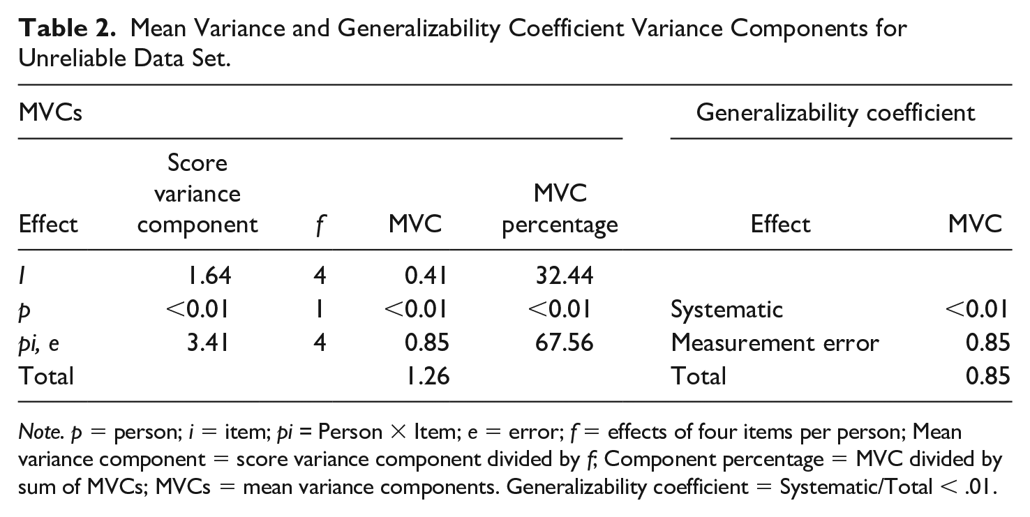
Note. p = person; i = item; pi = Person × Item; e = error; f = effects of four items per person; Mean variance component = score variance component divided by f; Component percentage = MVC divided by sum of MVCs; MVCs = mean variance components. Generalizability coefficient = Systematic/Total < .01.

After returning PER9 back to its original values, coefficient alpha and the generalizability coefficient increased to .77 [95% CI: 0.72, 0.81] and person produced the majority of the variance (75.48%) in the total MVC (see Table 3). As Thompson (2003) noted,

Having variance from people is a desirable outcome if our premise in a given study is that people differ as individuals, and that is exactly these differences that we wish to quantify or study. When we make such an assumption, we are defining people as our “object of measurement.” This assumption, in turn, means that we are defining all the variance due to the main effect of people as systematic or true variance, all other variances as measurement error variances. (p. 54)

Table 3.

Mean Variance and Generalizability Coefficient Variance Components for Corrected Data Set.

MVCs					Generalizability coefficient
Effect	Score variance component	f	MVC	MVC percentage	Effect	MVC
i	0.44	4	0.04	1.75
p	1.55	1	1.55	75.48	Systematic	1.55
pi, e	1.87	4	0.47	22.77	Measurement Error	0.47
Total			2.05		Total	2.01

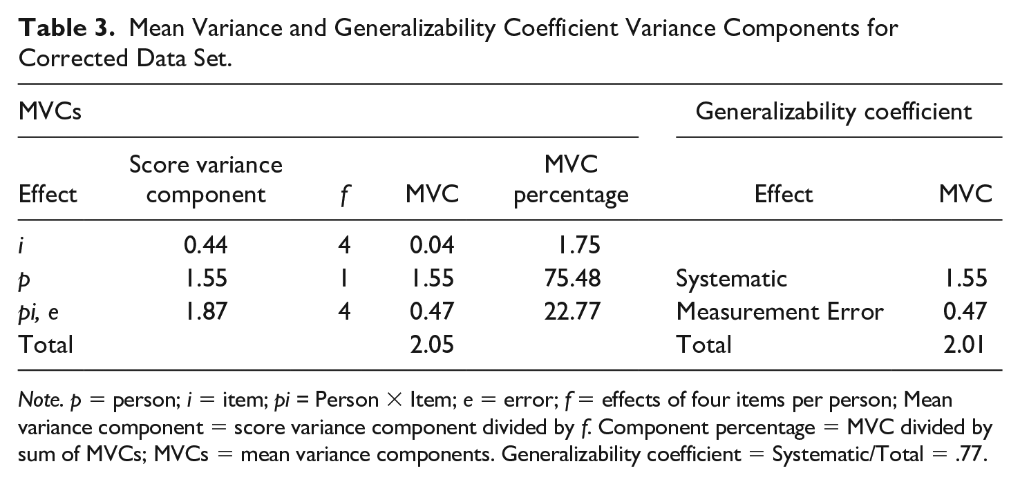
Note. p = person; i = item; pi = Person × Item; e = error; f = effects of four items per person; Mean variance component = score variance component divided by f. Component percentage = MVC divided by sum of MVCs; MVCs = mean variance components. Generalizability coefficient = Systematic/Total = .77.

Although all the reliability coefficients exceeded .70, we unbundled the sample to examine the robustness of the data and to determine if there were differences by role (i.e., graduate student vs. faculty) in keeping with Bernardi (1994). As seen in Table 4 and Figure 1, reliability increases to .80 [95% CI: 0.7, 0.84], the benchmark offered by Henson (2001) and others, when the 10 responses to the IA scale that yielded TAD values greater than 18 were eliminated.

Table 4.

Alpha and Mean Bootstrapped Alpha by Total Absolute Difference for Illustrative Example.

Sample results							Bootstrap results across 1,000 samples
α	CI_lower	CI_upper	TAD	N	n _Grd	n _Fac	M	SE	CI_lower	CI_upper
1.00	1.00	1.00	0	6	5	1
0.97	0.96	0.98	4	50	32	18	0.97	0.015	0.92	0.99
0.88	0.84	0.91	9	118	65	53	0.87	0.041	0.77	0.93
0.84	0.80	0.87	13	163	83	80	0.83	0.032	0.76	0.88
0.80	0.76	0.84	18	190	95	95	0.79	0.032	0.72	0.85
0.77	0.72	0.81	22	200	100	100	0.76	0.034	0.69	0.82

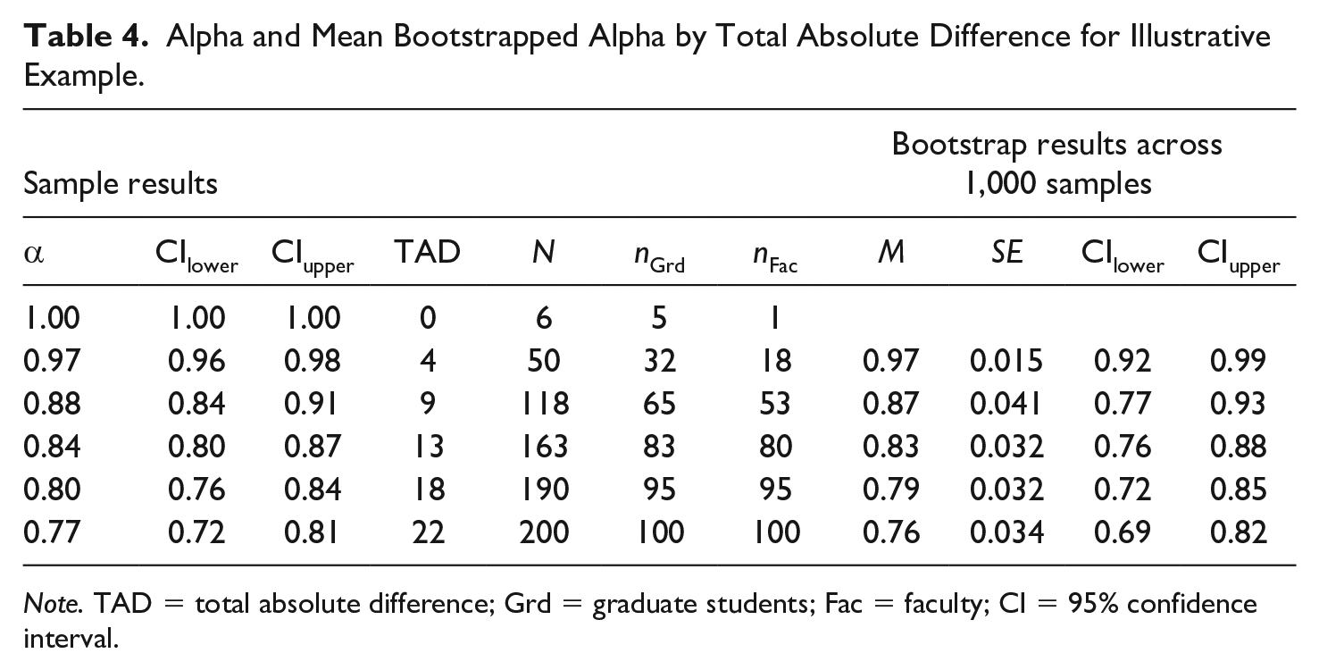
Note. TAD = total absolute difference; Grd = graduate students; Fac = faculty; CI = 95% confidence interval.

Figure 1.

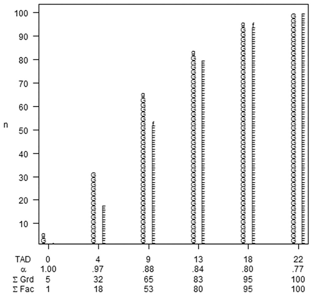
Total absolute difference (TAD) by alpha.

One can also see that graduate students appeared to yield higher alphas than faculty members, which was confirmed by calculating coefficient alpha for both groups where alpha for graduate students was .83 [95% CI: 0.78, 0.87] as compared with alpha of .68 [95% CI: 0.59, 0.77] for faculty. This difference in coefficient alpha by role is indicative of a measurement invariance issue (cf. Nimon & Reio, 2011).

Note that the bootstrap results are similar to the sample results. Although the mean bootstrapped coefficient alpha for the individuals who had a TAD value less than or equal to 18 (i.e., .79) did not meet the benchmark of .80 that was exhibited in the sample, the bootstrapped reliability estimate for the reduced sample is more replicable than the bootstrapped reliability estimate for the full sample (i.e., .032 < .034).

Discussion

With the limited information α < .70, the researcher is blind to the source of variance, and accordingly, correcting for a low coefficient alpha is merely trial and error. As we have demonstrated, G theory decomposes score variance and compartmentalizes it by source. With this information, the researcher can make an informed decision on how to proceed with the study rather than playing a guessing game.

After correcting for an item that had been erroneously reverse coded, the MVC for pi, e accounted had the highest error component percentage. To correct for the measurement error due to the interaction between person and item, we facilitated a process to eliminate subjects based on the largest TAD, following Bernardi (1994). Note that there is not a cut-off TAD value. It is up to researcher judgment to determine how many response sets to eliminate to achieve a desired alpha.

While we found the method of using TAD to be effective in understanding the relationship between coefficient alpha and sample subsets, a thorough investigation of the literature suggested that no researcher since Bernardi’s publication, 24 years ago, has approached low reliability using this procedure. Perhaps this is because, until now, statistical software did not provide the syntax to make the analysis user-friendly.

There is a misconception among scholars, that when coefficient alpha is below the acceptable range, item deletion is the only solution. However, deleting items may increase coefficient alpha to the detriment of content validity. As a result, the scale may not measure what it is intended to measure (Tavakol & Dennick, 2011). As well, if items are dropped, it may not be possible to compare the reliability coefficients from a reduced item set to reliability coefficients from other studies, as is done in reliability generalization studies (see Vacha-Haase, 1998), unless of course other researchers have eliminated the same set of items (cf. Helms et al., 2006).

Our proposed method demonstrated how to increase the reliability of data with a large measurement error without eliminating items and thus maintaining the integrity of the scale. One could argue that eliminating a small percentage of subjects is worthwhile if doing so maintains the integrity of the scale. Although deleting subjects could result in less representativeness of the population and generalizability of the study results (Kukull & Ganguli, 2012), such losses must be compared with the loss in content validity when a sample-specific set of items are used to measure a construct. In the end, it is up to researcher to make the appropriate tradeoffs including considering publication bias that may result from the file drawer problem if the study is not published because of issues with data reliability.

We would be remiss if we did not discuss the importance of transparency in reporting data. Scholars have a responsibility to maintain the rigor in the HRD literature. For test replication, items, or subjects that are eliminated, must be explained, and the coefficient alpha and effect size before and after the elimination should be reported along with support for the elimination decisions.

Limitations and Future Research

The limitations of this guide should be considered with the guidance provided herein. Our goal was to demonstrate a nonfile drawer approach to responding to low coefficient alpha. Although we believe the G theory analysis to be a valuable tool for assessing the source of error variance, it is the only approach this guide demonstrated. Furthermore, limited to the G study of a one-facet design, only a fraction of the uses of G theory was discussed. Second, while we feel that the purpose of this article was met, not all methods for correcting for low coefficient alpha were discussed. For example, collecting additional data or adding items to the measure may increase coefficient alpha. As it relates to the later, readers are cautioned that the effect of adding items to increase alpha may have a plateau effect. For example, Peterson (1994) found that coefficient alpha did not “appear to systematically increase once there were more than three items in a scale” (p. 390). Even though we maintain that eliminating a small percentage of subjects is favorable to deleting items, removing items may increase alpha. Third, as noted by Henson (2001), score reliability usually attenuates effect size, an important concept that was not addressed in this guide. Consideration of an instructional analysis detailing the process of correcting effect sizes for score reliability would facilitate rigor in HRD research. Based on these limitations, it is expected that not all research data will be saved from the file drawer following the procedures described here. Fourth, we did not explore how data characteristics relate to TAD values. For example, we did not explore how outlying responses influence TAD values. Finally, the consequences and remedies of high coefficient alpha remained untouched. A future primer outlining the issues related to high coefficient alpha (>.95) could be beneficial.

Implications

We believe that we have contributed to the HRD community by demonstrating a technique that may keep research that may otherwise remain unexplored out of the file drawer. Increasing the number of manuscripts published is knowledge shared that benefits scholars and practitioners alike. This demonstration provided an easy to follow guide for establishing data reliability in a study. By expanding the quantitative knowledge of scholars and practitioners, we empower our colleagues to move HRD research and theory building forward. It seems possible that with transparent reporting of results, the process of moving forward when coefficient alpha is low could strengthen empirical research that aims to explore or test theory. It would seem that much more could be learned from the published results of a subsample of data than an entire set of data that has been privately filed away. Furthermore, we are hopeful that our work will be an accessible resource for scholars who encounter data with low coefficient alpha.

Footnotes

Appendix

Declaration of Conflicting Interests

The author(s) declared no potential conflicts of interest with respect to the research, authorship, and/or publication of this article.

Funding

The author(s) received no financial support for the research, authorship, and/or publication of this article.

ORCID iD

Janice Lambert Chretien

Author Biographies

Janice Lambert Chretien is a doctoral candidate in the Department of Human Resource Development at The University of Texas at Tyler. Her research embraces instructional design, learning transfer, memory, and neurodiversity. She has 17 years as a training and career management director.

Kim Nimon, PhD, is associate professor in the Department of Human Resource Development at The University of Texas at Tyler. Her areas of expertise are in workforce development and quantitative analytical methods. She was awarded the Early Career Scholar Award by the Academy of Human Resource Development in 2013 and the Highly Commended Paper by Emerald Publishing in 2015 and currently serves as the external evaluator for several NSF funded projects.

Thomas G. Reio, Jr. is Professor of Adult Education and Human Resource Development at Florida International University in Miami, Florida. He is Editor of Human Resource Development Quarterly, and past editor of Human Resource Development Review and New Horizons in Adult Education and Human Resource Development. His research concerns curiosity and risk-taking motivation, workplace socialization processes, workplace incivility, entrepreneurship, and workplace learning. His work has been published in leading journals in education, business, and psychology. These journals include Personality and Individual Differences, The Journal of School Psychology, Educational and Psychological Measurement, Journal of Business and Psychology, Journal of Interpersonal Violence, Human Resource Development Quarterly, Human Resource Development International, Journal of Management Development, and the Journal of School Psychology. He has over 16 years of experience as a training and development director, organizational consultant, and operations manager.

Julie Roberts Lewis has worked as a consultant in a variety of industries including healthcare, high technology, automotive, chemical manufacturing, and transportation as an Environmental Manager & Compliance Auditor. She received her M.B.A. in General Business from Texas Woman’s University (2013) and Ph.D. in Organizational Development & Change from The University of Texas at Tyler (2019) while pursuing a full-time career as Global Environmental Manager in the oil and gas industry. She recently transitioned into the Human Resources function to focus on assessing and enhancing employee experiences throughout their employment life cycle. Her research interests include quality of work life (QOWL), organizational commitment, and voluntary turnover.

References

Baker

Turner

J. R.

Yoon

H. J.

Kwon

(Eds.). (2019). Examination of theoretical foundation: Implications for HRD research. Advances in Developing Human Resources, 21, 283–400.

Bates

Maechler

Bolker

Walker

(2019). lme4: Linear mixed-effects models using “eigen” and S4. https://cran.r-project.org/web/packages/lme4/index.html

Bernardi

R. A.

(1994). Validating research results when Cronbach’s alpha is below 0.70: A methodological procedure. Educational and Psychological Measurement, 54, 766–775. https://doi.org/10.1177/0013164494054003023

Bonett

D. G.

Wright

T. A.

(2015). Cronbach’s alpha reliability: Interval estimation, hypothesis testing, and sample size planning. Journal of Organizational Behavior, 36, 3–15. https://doi.org/10.1002/job.1960

Bosco

(2018). File drawer problem. In Frey

B. B.

(Ed.), The Sage encyclopedia of educational research, measurement, and evaluation (Vols. 1–4, pp. 677–678). SAGE. https://doi.org/10.4135/9781506326139

Brown

J. D.

(2018). Spearman-Brown prophecy formula. In Frey

B. B.

(Ed.), The Sage encyclopedia of educational research, measurement, and evaluation. SAGE. https://doi.org/10.4135/9781506326139

Canty

Ripley

(2019). boot: Bootstrap R (S-PLUS) functions (R package version 1.3-22).

Chalofsky

(2007). The seminal foundation of the discipline of HRD: People, learning, and organizations. Human Resource Development Quarterly, 18, 431–442. https://doi.org/10.1002/hrdq.1212

Cook

Thompson

(2001). Psychometric properties of scores from the web-based LibQUAL+ study of perceptions of library service quality. Library Trends, 49, 585–603.

10.

Cortina

J. M.

(1993). What is coefficient alpha an examination of theory and applications. Journal of Applied Psychology, 78, 98–104.

11.

Cronbach

L. J.

(1951). Coefficient alpha and the internal structure of tests. Psychometrika, 16, 297–334. https://doi.org/10.1007/BF02310555

12.

Cronbach

L. J.

Gleser

G. C.

Nanda

Rajaratnam

(1972). The dependability of behavioral measurements: Theory of generalizability for scores and profiles. John Wiley & Sons.

13.

Cronbach

L. J.

Rajaratnam

Gleser

G. C.

(1963). Theory of generalizability: A liberalization of reliability theory. British Journal of Statistical Psychology, 16, 137–163. https://doi.org/10.1111/j.2044-8317.1963.tb00206.x

14.

Cronbach

L. J.

Shavelson

R. J.

(2004). My current thoughts on coefficient alpha and successor procedures. Educational and Psychological Measurement, 64, 391–418. https://doi.org/10.1177/0013164404266386

15.

Edwards

J. M.

Finch

W. H.

(2018). Missing data analysis. In Frey

B. B.

(Ed.), The Sage encyclopedia of educational research, measurement, and evaluation. SAGE. https://doi.org/10.4135/9781506326139

16.

Enders

C. K.

(2004). The impact of missing data on sample reliability estimates: Implications for reliability reporting practices. Educational and Psychological Measurement, 64, 419–436. https://doi.org/10.1177/0013164403261050

17.

Enders

C. K.

Bandalos

D. L.

(1999). The effects of heterogeneous item distributions on reliability. Applied Measurement in Education, 12, 133–150. https://doi.org/10.1207/s15324818ame1202_2

18.

Fan

Thompson

(2001). Confidence intervals for effect sizes: Confidence intervals about score reliability coefficients, please: An EPM guidelines editorial. Educational and Psychological Measurement, 61, 517–531. https://doi.org/10.1177/0013164401614001

19.

Field

A. P.

Miles

Field

(2012). Discovering statistics using R. SAGE.

20.

Fox

Weisberg

Price

(2018). car: Companion to applied regression. https://cran.r-project.org/web/packages/car/index.html

21.

Gill

M. J.

(2017). Outlier analysis. In Allen

(Ed.), The Sage encyclopedia of communication research methods. SAGE. https://doi.org/10.4135/9781483381411

22.

Greco

L. M.

O’Boyle

E. H.

Cockburn

B. S.

Yuan

(2018). Meta-analysis of coefficient alpha: A reliability generalization study. Journal of Management Studies, 55, 583–618. https://doi.org/10.1111/joms.12328

23.

Gronlund

N. E.

Linn

R. L.

(1990). Measurement and evaluation in teaching (6th ed.). Palgrave Macmillan.

24.

Heider

(1958). The psychology of interpersonal relations. John Wiley & Sons.

25.

Helms

J. E.

Henze

K. T.

Sass

T. L.

Mifsud

V. A.

(2006). Treating Cronbach’s alpha reliability coefficients as data in counseling research. The Counseling Psychologist, 34, 630–660. https://doi.org/10.1177/0011000006288308

26.

Henson

R. K.

(2001). Understanding internal consistency reliability estimates: A conceptual primer on coefficient alpha. Measurement and Evaluation in Counseling and Development, 34, 177–189. https://doi.org/10.1080/07481756.2002.12069034

27.

Kaplan

R. W.

Saccuzzo

D. P.

(1982). Psycological testing: Principles, applications, and issues. Brooks/Cole.

28.

Kelly

H. H.

(1992). Common-sense psychology and scientific psychology. Annual Review of Psychology, 43, 1–23.

29.

Kopalle

P. K.

Lehmann

D. R.

(1997). Alpha inflation? The impact of eliminating scale items on Cronbach’s alpha. Organizational Behavior and Human Decision Processes, 70, 189–197. https://doi.org/10.1006/obhd.1997.2702

30.

Kuder

G. F.

Richardson

M. W.

(1937). The theory of the estimation of test reliability. Psychometrika, 2, 151-160. https://doi.org/10.1007/BF02288391

31.

Kukull

W. A.

Ganguli

(2012). Generalizability: The trees, the forest, and the low-hanging fruit. Neurology, 78(23), 1886–1891. https://doi.org/10.1212/WNL.0b013e318258f812

32.

McNeish

(2018). Thanks coefficient alpha, we’ll take it from here. Psychological Methods, 23, 412–433. https://doi.org/10.1037/met0000144

33.

Multon

K. D.

Coleman

J. S. M.

(2010). Coefficient alpha. In Salkind

N. J.

(Ed.), Encyclopedia of research design. SAGE. https://doi.org/10.4135/9781412961288.n53

34.

Murphy

K. R.

Davidshofer

C. O.

(1988). Psychological testing: Principles and applications. Prentice-Hall.

35.

Nimon

Oswald

Roberts

J. K.

(2013). yhat: Interpreting regression effects (package version 2.0-5). https://rdrr.io/cran/yhat/man/yhat-package.html

36.

Nimon

Reio

T. G.

Jr (2011). Measurement invariance: A foundational principle for quantitative theory building. Human Resource Development Review, 10, 198–214. https://doi.org/10.1177/1534484311399731

37.

Nimon

Reio

T. G.

Shuck

(Eds.). (2015). Quantitative data-analytic techniques to advance HRD theory and practice. Advances in Developing Human Resources, 17(1), 1–134.

38.

Nunnally

J. C.

(1967). Psychometric theory. McGraw-Hill.

39.

Nunnally

J. C.

(1978). Psychometric theory (2nd ed.). McGraw-Hill.

40.

Peterson

R. A.

(1994). A meta-analysis of Cronbach’s coefficient alpha. Journal of Consumer Research, 21, 381-391. doi:10.1086/209405

41.

Raykov

(2007). Reliability if deleted, not ‘alpha if deleted’: Evaluation of scale reliability following component deletion. British Journal of Mathematical and Statistical Psychology, 60, 201–216. https://doi.org/10.1348/000711006X115954

42.

R Development Core Team. (2019). R: A language and environment for statistical computing [Computer software]. R Foundation for Statistical Computing. http://www.R-project.org/

43.

Reinard

J. C.

(2006). Communication research statistics. SAGE. https://doi.org/10.4135/9781412983693

44.

Revelle

(2019). psych: Procedures for psychological, psychometric, and personality research. https://cran.r-project.org/web/packages/psych/index.html

45.

Schmidt

F. L.

Hunter

J. E.

(2014). Methods of meta-analysis: Correction-error and bias in research findings (3rd ed.). SAGE.

46.

Schmitt

(1996). Uses and abuses of coefficient alpha. Psychological Assessment, 8, 350–353. https://doi.org/10.1037/1040-3590.8.4.350

47.

Shavelson

R. J.

Webb

Rowley

(1989). Generalizability theory. American Psychologist, 44, 922–932. https://doi.org/10.1037/0003-066X.44.6.922

48.

Shavelson

R. J.

Webb

N. M. W.

(1981). Generalizability theory: 1973-1980. British Journal of Mathematical and Statistical Psychology, 34, 136–166. https://doi.org/10.1111/j.2044-8317.1981.tb00625.x

49.

Song

J. H.

Lim

D. H.

(2015). Mediating analysis approaches: Trends and implications for advanced applications in HRD research. Advances in Developing Human Resources, 17, 57–71. https://doi.org/10.1177/1523422314559807

50.

Tavakol

Dennick

(2011). Making sense of Cronbach’s alpha. International Journal of Medical Education, 2, 53–55. https://doi.org/10.5116/ijme.4dfb.8dfd

51.

Thompson

(2003). Score reliability: Contemporary thinking on reliability issues. SAGE.

52.

Thompson

(2004). Exploratory and confirmatory factor analysis: Understanding concepts and applications. American Psychological Association.

53.

Thompson

Cook

Heath

F. M.

(2001). How many dimensions does it take to measure users’ perceptions of libraries? A LibQUAL+ study. Portal: Libraries and the Academy, 1, 129–138. https://doi.org/10.1353/pla.2001.0030

54.

Thompson

Cook

Thompson

R. L.

(2002). Reliability and structure of LibQUAL+ scores: Measuring perceived library service quality. Portal: Libraries and the Academy, 2, 3–12. https://doi.org/10.1353/pla.2002.0022

55.

Thompson

Daniel

(1996). Seminal readings on reliability and validity: A “hit parade” bibliography. Educational and Psychological Measurement, 56, 741–745.

56.

Thompson

Vacha-Haase

(2000). Psychometrics is datametrics: The test is not reliable. Educational and Psychological Measurement, 60, 174–195. https://doi.org/10.1177/0013164400602002

57.

Vacha-Haase

(1998). Reliability generalization: Exploring variance in measurement error affecting score reliability across studies. Educational and Psychological Measurement, 58, 6–20.

58.

Van Ginkel

J. R.

Van der Ark

L. A.

Sijtsma

. (2007). Multiple imputation of item scores in test and questionnaire data, and influence on psychometric results. Multivariate Behavioral Research, 42, 387–414. https://doi.org/10.1080/00273170701360803

59.

Webb

N. M.

Shavelson

R. J.

(2005). Generalizability theory: Overview. Encyclopedia of Statistics in Behavioral Science, 2, 717–719.

60.

Webb

N. M.

Shavelson

R. J.

Haertel

E. H.

(2006). 4 Reliability coefficients and generalizability theory. Handbook of Statistics, 26, 81–124. https://doi.org/10.1016/S0169-7161(06)26004-8

61.

Wilkinson

, Task Force on Statistical Inference, American Psychological Association, & Board of Scientific Affairs. (1999). Statistical methods in psychology journals. American Psychologist, 54, 594–604. https://doi.org/10.1037/0003-066x.54.8.594

62.

Worthington

R. L.

Whittaker

T. A.

(2006). Scale development research: A content analysis and recommendations for best practices. The Counseling Psychologist, 34, 806–838. https://doi.org/10.1177/0011000006288127