Spatial clustering: Influence of urban street networks on retail sales volumes

Abstract

As is often believed that the more centrally located a shop, the higher its sales volume, this paper analyzed relationships between the spatial clustering of retail stores, their respective transaction volumes, and the urban street networks to determine whether, and to what extent, the accessibility and density of a store’s location was correlated with its transaction volume. While this hypothesis is widely accepted, its veracity is underexplored and rarely validated using large-scale empirical datasets, possibly owing to the lack of access. Therefore, transaction datasets and accessibility indicators were first examined; a clear, positive correlation between density and revenue was found for specialty stores wherein people do “comparison shopping,” and for stores that complemented each other for activities such as “one-trip shopping,” the revenues were positively correlated when the stores were clustered. Generally, daily-use stores’ revenues were more sensitive to local access and those of non-daily-use stores were more sensitive to global access. In conclusion, these findings would not have been found using conventional methodology focused on the retail sector as a whole, because aggregate market mechanisms would have hidden the observed effects on specific store categories. Therefore, upon disaggregating the data, we found a distinct heterogeneity across the different store types for what concerns the relationship between revenue and location.

Keywords

Complex street networks urban morphology centrality transaction data

Introduction

City spatial configurations and the relationships with social behavior have been researched in fields ranging from urban planning to the social and economic sciences (Albert and Barabási, 2002; Barabási and Albert, 1999; Fujita and Thisse, 2013; Hillier, 1996; Hillier and Hanson, 1984; Jiang et al., 2014; March and Steadman, 1971; Martin and March, 1972; Porta et al., 2006b, 2009, 2012; Sevtsuk, 2014; Watts and Strogatz, 1998). Previous studies found cities as tending to have similar geometric patterns and features (Barthélemy and Flammini, 2008; Bohn et al., 2002; Lämmer et al., 2006; Masucci et al., 2014; Perna et al., 2011; Strano et al., 2013). Spatial graph primal representations (Porta et al., 2006b) are used to analyze accessibility and centrality in urban topologies, observing different distributions of centrality values between a self-organized, historical development city and predominantly planned city developments (Barthélemy et al., 2013; Cardillo et al., 2006; Crucitti et al., 2006; Lämmer et al., 2006; Porta et al., 2006b). While urban street networks through the primal approach cannot capture the underlying scaling property of streets because nodes and edges are embedded in the three-dimensional Euclidean space (Ma et al., 2019), spatial graph dual representations (Porta et al., 2006a) find the nontrivial small-world and scale-free topological properties that a relatively small number of streets tend to play dominant roles in city structures (Jiang, 2007; Jiang and Claramunt, 2004; Kang et al., 2016; Masucci et al., 2014). Spatial economics, however, examines the mechanisms and rules behind spatial agglomerations at the city, regional, national, and international levels (Fujita and Thisse, 2013), with the distribution of the economic activities and their spatial clustering considered a result of a trade-off between various forces (e.g. centripetal force and centrifugal force). For example, the physical proximity of economic entities facilitates communication and overcomes the information distance decay resulting in externalities (Lucas, 1988). However, excessive density in geographically limited areas decreases comfort and satisfaction, making the centrifugal forces stronger. Therefore, based on the self-organizing, bottom-up processes typical of complex systems, these mutual interactions would be expected to affect both the appearance and shape of cities (Fujita and Thisse, 2013; Krugman, 1996).

However, despite extensive research, few studies have combined spatial configurations and land use location choices at the neighborhood/street resolution level. For instance, retail location theory has rarely dealt with exogenous factors such as the geometric elements in the built environment, and architects and urban planners have seldom considered previous urban economic data (Sevtsuk, 2010: 12, 2014: 374). Unfortunately, most prominent models combining spatial and human behavioral dimensions have been based on strong but simplified assumptions (Alonso, 1964; Christaller and Baskin, 1966; DiPasquale and Wheaton, 1996; Huff, 1963; Lösch, 1954; Mills, 1967; Muth, 1969; Von Thünen, 1826). Overall, “it is rare to find an economics text in which space is studied as an important subject – if it is even mentioned” (Fujita and Thisse, 2013: 11).

To bridge the theoretical gap between configurational and human behavioral models and provide a more definite, quantitative understanding of how specific locational features may or may not influence citizen behavior, this paper analyzed the distribution of economic activities at a fine spatial resolution that considered the spatial configuration of the built environment. Both the spatial clustering of small-scale retail stores and their density at the neighborhood scale were considered along with the centrality metrics of the road network. Although few similar studies were conducted owing to the need for extensive observations of both spatial and human behavioral choices in the same urban configuration, there are now better opportunities for the acquisition and analysis of human and urban behavior data because of the emerging field of big data analysis (Yoshimura et al., 2018).

The specific question addressed in this study was related to retail location theory; namely, whether and to what extent a shop’s success, measured here as its sales volume, was related to its location in the city. Different location measures, such as local density, shop clustering, and a centrality metric, were considered in the analysis to gauge shop accessibility. As is customary in retail and urban planning studies (Porta et al., 2009), the hypothesis driving this study was that more centrally located shops and/or those spatially clustered with other shops are more successful than less accessible shops. While this hypothesis is the same as in past research (Hillier, 1996; Porta et al., 2009, 2012) that looked at the correlations between the centrality and retail and service densities, the exploration in this paper focuses on the correlations between store revenues, store clustering, and geolocations leveraging massive datasets of economic activities and street network from Barcelona, Spain.

Analytical framework

The analytical methodological framework had two main steps: the first step was to statistically test whether the store locations and revenues were clustered. To do this, the observed store locations were compared with the same number of randomly distributed stores (see section 2 in the supplementary material for detail). If the store proximities were closer than those perceived in the randomly distributed sample, it was assumed that the stores’ cluster pattern at the location was not formed by chance. As our driving hypothesis was that geographical advantage attracted many stores to cluster in specific locations in the city, which would possibly have higher revenues than those located on periphery, the second step was to explore the relationship between street network centrality and cluster locations using Porta et al.’s (2009) methodology. In other words, an estimated density centrality value computed the cell-by-cell correlations with the estimated retail activity density values. Therefore, this paper explored and accurately quantified the correlations between the clustered locations, the respective higher sales volumes, and the central locations through the analysis of large quantities of data.

Spatial scale distances

Definitions for the basic aggregation unit and other scale parameters are fundamental to spatial analysis as the spatial clusters and associated strengths could be significantly different depending on the geographical and spatial scale used (Fujita and Thisse, 2013). As the hypotheses were that retail store location choice depended on the (road) network distance and locational spatial accessibility, and that various retail stores had different network size preferences for their target customers, the following distances were defined as the spatial scale for the analysis

d = (300 m, 400 m, 500 m, \dots, 5000 m, increased by 1 00 m)

grid_d = (10 m, 20 m, 30 m, \dots, 250 m, increased by 1 0 m)

moran_d = (50 m, 60 m, 70 m, \dots, 1000 m, increased by 1 0 m)

where d was the (road) network distance from a reference node i in the road graph G used in this analysis, and grid distance, grid_d, was applied to set the grid size for the kernel density estimation (KDE). The study area was divided into square cells of equal size in grid_d, which changed from 10 to 250 m in steps of 10 m. The objective of these changes was to assess the robustness of the analysis; that is, to what extent the spatial aggregation unit influenced the results. The kernel function’s bandwidth was fixed at 300 m, corresponding to a five-minute walking distance. Finally, the moran_d distance was applied to compute the global Moran’s I and Getis–Ord Gi* indexes.

Global Moran’s I and Getis–Ord Gi*

The retail store spatial autocorrelation was examined as the first law of geography because “Everything is related to everything else but near things are more related than distant things” (Tobler, 1970: 236). Therefore, physically proximate stores were more likely to form clusters than stores further away from each other. The global Moran’s I index (Anselin, 1988) measures the positive or negative spatial correlation and its strength, comparing the observed economic activity distributions with the same number of hypothetically randomly distributed economic activities within the study area (see Figure S3). Moran’s I and associated methods are typically used to judge upon the existence of spatial clustering, but as they cannot quantify the clustering degree, the Getis–Ord Gi* (Getis and Ord, 1996; Ord and Getis, 1995) was used to measure the spatial clustering intensity in hotspot/coldspot locations (see Figure S4).

Centrality indicator

The betweenness centrality (Freeman, 1977) was computed to measure the local accessibility in the spatial networks, determined by examining the subset of nodes and edges in the network. Node i’s betweenness was determined using $C_{i}^{B d}$ to consider the network distance d; that is, the network distance d was changed from a neighborhood scale to a city scale for node i and a betweenness for every node i computed.

The applied methodology utilized the “edge effect,” generated using artificially bounded networks (Okabe and Sugihara, 2012: 41–42; Porta et al., 2006a: 715–718), to estimate the adequate network distance from the specific retail store locations. The betweenness indicator is sensitive to network form; that is, the number of nodes, how they are linked, and the boundaries. Although many researchers have proposed potential solutions to soften these effects (Gil, 2017), the characteristics of the edge effect were used here to identify the location clusters that had similar accessibility patterns.

Figure 1 shows the different network distances d for node i. Changing d to compute the betweenness for node i results in different scores for node i (see Figure 1(b) and (c)); the changes in node i’s betweenness scores during changes in the function of d were explored. Figure 1 shows the betweenness scores for different network distance d values: (a) 300 m, (b) 2000 m, and (c) 5000 m. In the smaller-scale network, the locations with higher betweenness scores were located on local arteries that connected public spaces at the neighborhood scale. The more accessible locations gradually changed as the network size increased and became more coincident with the large-scale inter-district avenues for the largest value of d (Figure 1(c)).

Figure 1.

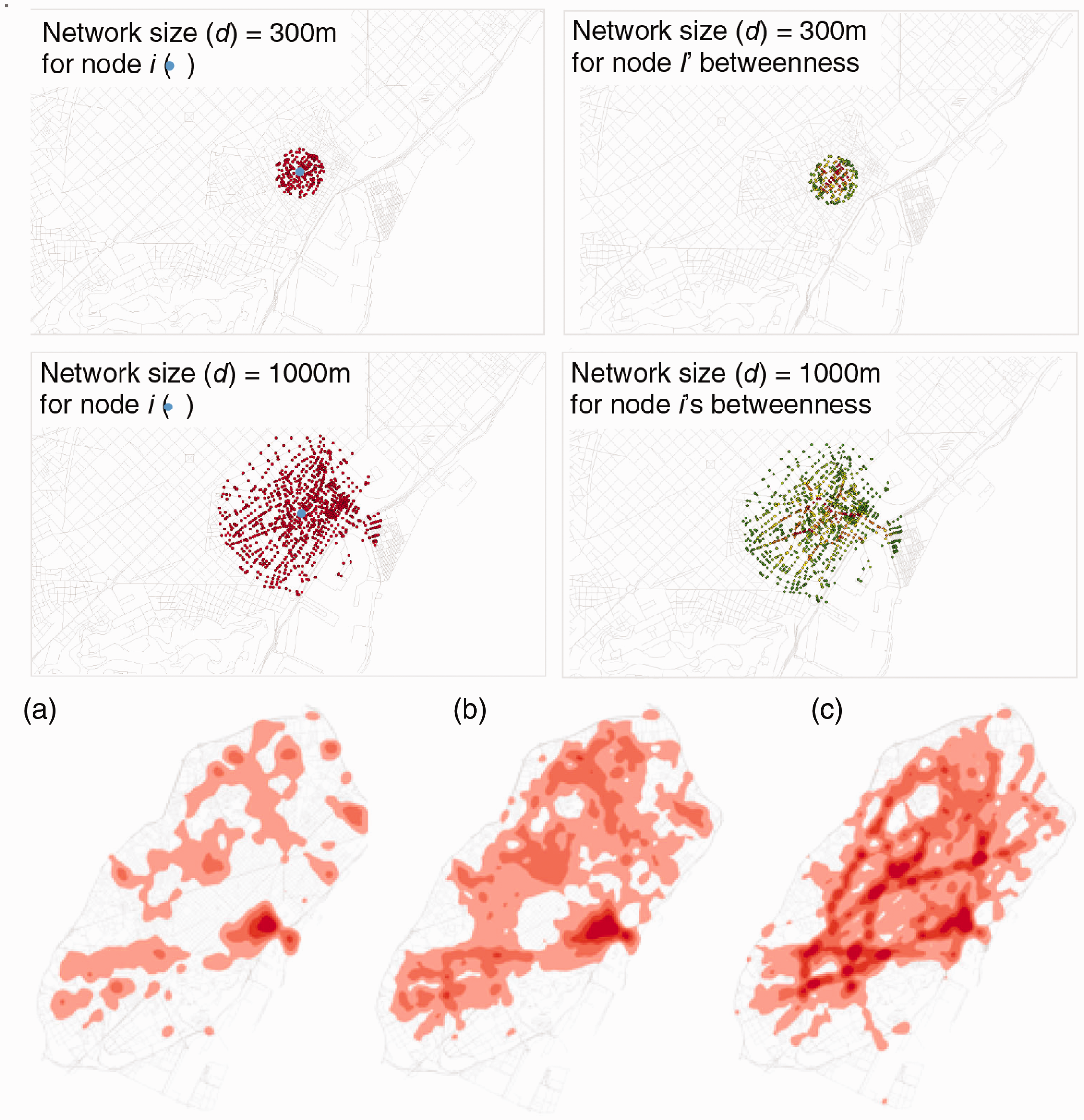
The different network sizes to be considered for node i and the difference in the results. The figure shows the betweenness scores for the different network distances d: (a) 300 m, (b) 2000 m, and (c) 5000 m, which respectively represent the neighborhood, district, and city scales. The darker red tones correspond to higher betweenness scores.

It was hypothesized that the smaller-scale network size (e.g. 300 m) would be useful for daily-use stores (e.g. butchers and supermarkets) because it suggests pedestrian access around the specific location at the neighborhood scale. The larger network size (e.g. 5000 m) may be more useful for non-daily-use stores (e.g. department stores) because it would be useful for vehicle-based access on a larger scale (e.g. district scale).

As different dependence patterns of betweenness as a function of d were found, to quantitatively identify the particular clusters, a silhouette test was first applied to determine the best number of clusters to use; then, the result was input to the k-means clustering algorithm. The silhouette test’s outcome indicated that the four k-means clusters were adequate (an average s-value = 0.51). The nodes in the first and second cluster were quite evenly distributed over the city, and the nodes in the third (locally important) and fourth clusters (important at city level) had clear spatial signatures (see Figure 2). The third cluster, which was the locally important nodes, was exclusively located in the historic center and corresponded to the arteries constructed at the beginning of the city formation. However, the nodes in the fourth cluster corresponded to the larger avenues that connected the different parts of the city.

Figure 2.

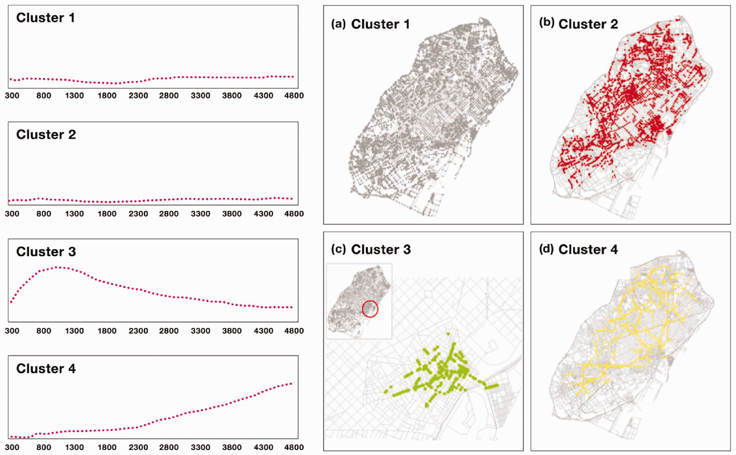
The representative distribution of nodes’ betweenness scores in the street network and its change by the network size, and their visualizations in the city (a–d).

The proposed clustering method effectively identified the nodes with different levels of importance in the city, and thus, the following analysis used these four clusters to study the possible correlations between economic activities and accessibility.

Kernel density estimation

KDE was applied to the correlation analysis. It enables the density of events (or objects) within a predefined radius to be computed as the average density around nearby locations, with the weights depending on the spatial distances. Figure S1 in the supplementary material shows a diagram of the KDE operations, wherein a kernel function is observed to determine the weights for each event as a function of the distances; the maximum value is at the center of the targeted grid square (point k in Figure S1 in the supplementary material) and becomes 0 at the end of the bandwidth (Fotheringham et al., 2000: 146–149), with the kernel density for point k in the grid being estimated as the sum of all weighted events within the bandwidth. The KDE results provide information about the density of events in a place based on the surrounding effects rather than on the individual store or entity because, as Porta et al. (2009) described, the focus is not the individual store; rather it is on what makes the environment special, which includes the nearby stores.

In this study, KDE was applied to the following variables

n k j

N k

c k j

C k

sv k j

SV k

csv k j

CSV k

C^{B d}

where nkj represented the KDE for the number of shops in category j in grid square k, Nk was the KDE for the number of shops in all categories in grid square k, ckj was the KDE for the z-score for the shops in category j in grid square k, Ck was the KDE for the z-score of the shops in all categories in grid square k, svkj was the KDE for the shops’ sales volumes in category j in grid square k, and SVk was the KDE of the stores’ sales volumes in all categories in grid square k. cvkj was the KDE of the z-score of the stores’ sales volumes in category j in grid square k, and CSVk was the KDE for the z-scores for the stores’ sales volumes in all categories in grid square k. KDE was also employed to compute the node accessibility scores for the street network based on the betweenness centrality

C^{B d}

, for which the ArcGIS’s built-in tool for KDE was also used.

Data description

The dataset was composed of a large number of transaction records made available to the researchers by a major Spanish bank, which consisted of debit or credit card transactions from the bank’s direct customers and transactions from the bank’s point of sale terminals around the country. The provided information included the shop wherein the customer made the transaction, transaction’s timestamp, and amount of money spent, as well as a unique ID for each customer’s credit or debit card that was not associated with the real customer ID or bank card. The data were aggregated and hashed for anonymization in accordance with local privacy protection laws and regulations.

The shops were originally classified into 76 categories; however, based on previous research on economic activities in Barcelona (Porta et al., 2012), the shops were manually reclassified into seven general categories and 17 sub-categories depending on whether they were primary or secondary activities (see Table 1 in Yoshimura et al. 2018: 19 for all categories). Therefore, the differences in the relationships between the locations and the sales volumes and between the primary and secondary activities were analyzed. The analysis was focused on categories A and B, which corresponded to most small-scale retail shops and services. The category and sub-category definitions for A and B and the primary and secondary activity classifications and the basic properties are given in the supplementary material in Table S1 and shown in Figure S2. The store–store relationship analysis considered whether the shops were “imperfect substitutes (comparison shopping)” or “complementary goods (one-trip shopping).”

Results

Spatial clustering quantification

Retail store spatial clustering

Figure 3(a) shows the Moran’s I index for the individual categories, from which it can be seen that all obtained scores had a p-value < 0.05 and a z-score > 2.56, which indicated that the stores in all individual categories were spatially autocorrelated and the clustering was statistically significant. As the Moran’s I index systematically decreased when the considered distance increased, it was surmised that the clustering effect was weaker when the considered distance became larger. Category B2 (hotels, hostels, and B&Bs) had the highest Moran’s I index at all distances, with the clustering effect being much stronger than the general category B (hotels, B&Bs, hostels, restaurants, cafés, and pubs), which suggested that the higher number of stores in the combined categories did not always result in higher clustering. This was consistent with the results shown in Figure 3(b), which shows the Moran’s I index for all possible combinations between the individual categories for A (eight categories) and B (five categories). Interestingly, individual category B’s addition helped increase some of the individual category A Moran’s I indexes, but not all.

Figure 3.

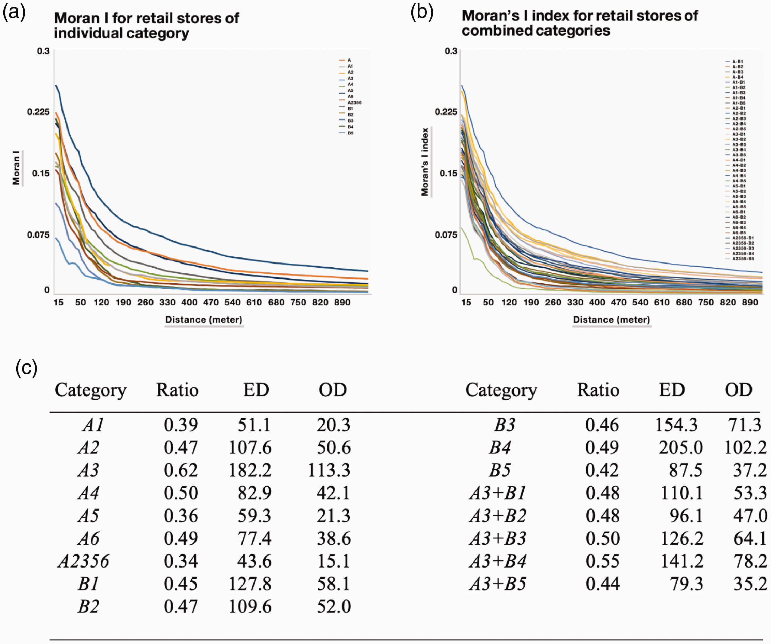
(a) Moran’s I index for individual categories and the change of values with the distance (moran_d). (b) Moran’s I index for the combined categories and the change of values with the distance (moran_d). (c) Table for the nearest neighbor analysis. ED: expected distance; OD: observed distance; OD/ED: ratio.

To examine the physical distance between each store in each category, a nearest neighbor analysis was performed (Mitchell, 2009), which compared the observed distance from the actual dataset and the expected distance if the same number of stores was iteratively and randomly distributed. Figure 3(c) shows that all nearest neighbor indexes were less than 1.0 (p < 0.05 and z-score < –2.56), indicating that all individual category retail stores were physically located much closer to each other than expected. The individual category, category A1 stores (grocery stores), were observed to be located the nearest to each other, and the observed distance for A3 was significantly improved when it was considered with an individual category B.

A hotspot and coldspot analysis was also conducted using Getis–Ord Gi*, which distinguished the locations based on clustering strength and indicated that it was possible to differentiate the densified areas from the locations wherein store agglomerations were statistically significant. The spatial clustering locations did not always coincide with the denser areas (see Figure S5 in the supplementary material as an example of category A1). Further, some hotspots did not correspond to the areas wherein the stores were highly agglomerated.

Figure S6 in the supplementary material shows the coefficient determinations ( $R^{2}$ ) between the store densities and the spatial clustering locations. Although all p-values in all $R^{2}$ categories were less than 0.05 (p < 0.05), $R^{2}$ was largely dependent on the categories; A2, B4, and A5 had higher correlations ( $R^{2}$ > 0.6) than the other categories, which had much lower $R^{2}$ values. For example, A6, A4, and A had correlations lower than 0.25, which suggested that the densified store areas did not match store spatial clustering locations.

These results, therefore, confirmed that the retail stores in each category were spatially clustered and such clustering was statistically significant. Moreover, the analysis showed that the spatial clustering locations were different from the high-store density areas. According to these results, an apparently denser area may not always indicate the most important clustering patterns in the city; thus, the proposed statistical spatial methodology revealed these important differences, which could be useful for retailers looking for the best locations.

Correlation analysis

Density of retail stores vs. sales volumes

Based on the spatial analyses in the previous section, the sales volumes in the higher-density areas and spatial clustering locations were further explored using the $R^{2}$ correlation analysis on the following variable pairs to test the hypothesis that a larger store agglomeration contributes to higher sales volumes

R^{2} (N k, sv k j)

R^{2} (C k, csv k j)

R^{2} (n k j, sv k j)

R^{2} (c k j, csv k j)

Although all p-values were less than 0.05, the $R^{2}$ analysis found all low scores (see Figure S7(a) and (b) in the supplementary material), indicating that neither the all category store density nor the spatial clustering locations could explain the individual category sales volume density or the spatial clustering of the sales volumes. This is an intriguing result because, generally, when a larger number of stores are agglomerated, there is a larger revenue volume. Furthermore, the $R^{2}$ analysis showed that having other store types in the surrounding environment did not necessarily assist in increasing a specific category’s sales volumes; that is, a specific category’s revenue appeared to be independent of the density and spatial clustering of all categories.

However, when focusing on individual category as the factor for the $R^{2}$ , the result was different. Figure S7(c) in the supplementary material shows that $R^{2}$ (skB2, nkB2; hotels, hostels, and B&Bs) and $R^{2}$ (sk(A3 + B2 and ck A3 + B2; personal equipment such as jewelry and watches + hotels, and hostels, and B&Bs) had higher scores and were statistically significant ( $R^{2}$ = 0.64, p < 0.01, $R^{2}$ = 0.57, p < 0.01). While the higher store density in category A3 was found to be unrelated to an increase in sales volume, when combined with the category B2 results, there were noticeably higher sales volumes. The previous section showed that personal equipment stores (e.g. jewelry and watches) tended to be located nearer to hotels; however, this analysis revealed that their presence in a denser area could also explain the higher sales volumes.

Figure S7(d) in the supplementary material also shows that the coefficient determination ( $R^{2}$ (ckA3, csvkA3), $R^{2}$ (ck(A3 + B4), csvk(A3 + B4))) had higher values ( $R^{2}$ = 0.61, p < 0.01, $R^{2}$ = 0.60, p < 0.01), indicating the spatial clustering of these stores could explain the spatial clustering of their respective sales volumes. This was in line with Eaton and Lipsey (1982), who found people may compare similar products and prices in nearby stores before making purchase decisions, especially when considering luxury personal goods such as jewelry. Therefore, while consumers may benefit from lower search and transportation costs and higher savings because of the stores’ proximities, retailers could also expect an increase in potential customers and demand externalities due to customer spillovers from other stores in the same cluster. These findings also suggested that the spatial clustering location of A3 + B4 could explain the spatial clustering of their higher sales volumes. Therefore, it is speculated that as people may visit cafés (category B4) before or after purchasing items from a category A3 store, these two categories are likely to be located in the same cluster to take advantage of the economic synergy.

Correlations between locational density, spatial clustering, revenues, and centrality scores

The previous sections revealed that (1) the spatial clustering of retail stores was derived from their spatial autocorrelation (Spatial Clustering Quantification section) and (2) neither the highly densified store locations nor the highly clustered locations coincided with places producing higher sales volumes. However, the highly densified areas in categories B2 and A3 + B2 could explain the high density of their sales volumes, and the spatial clustering locations of A3, A3 + B4, and A3 + B3 could explain the spatial clustering of their higher sales volumes. Therefore, based on these findings, this section examined whether, and to what extent, the clustering locations were correlated with the central places based on the street network to determine whether better spatial accessibility could explain the spatial clustering of retailers and their higher sales volumes.

To analyze this correlation, the $R^{2}$ coefficient was computed between the betweenness scores and (1) the density of retail stores, (2) their spatial clustering locations, (3) the density of the store sales volumes, and (4) the spatial clustering of the store sales volumes; that is, $R^{2}$ ( $C^{B d}$ , nkj), $R^{2}$ ( $C^{B d}$ , ckj), $R^{2}$ ( $C^{B d}$ , svkj), and $R^{2}$ ( $C^{B d}$ , cvkj) where d (=300, 400, 500, …, 5000), grid_d (=10, 20, 30, …, 250), and j (=A, A1, A2, …, A3, B5).

$R^{2}$ was independent of grid size from 10 to 250 m, which further confirmed the analytical methodology’s robustness (see section 3.4 in the supplementary material). All p-values up to a 250 m grid size were less than 0.01, indicating that the correlation was statistically significant. All $R^{2}$ values were below 0.5, which was relatively low, with the $R^{2}$ values for density (Figure S8(a) in the supplementary material) being higher than for spatial clustering (Figure S8(b) in the supplementary material), which indicated that the densified store areas and spatial clustering locations were largely independent of road accessibility.

The $R^{2}$ between the betweenness scores and (1) the density of stores’ sales volumes ( $R^{2}$ ( $C^{B 5000}$ , svkj)) and (2) the spatial clustering of the store sales volumes ( $R^{2}$ ( $C^{B 5000}$ , cvkj)) were also computed. Figure S8(c) and (d) in the supplementary material shows that all $R^{2}$ values were below 0.1 except A3 + B3 ( $R^{2}$ = 0.10 with p < 0.05). The coefficient determination for the spatial clustering for the store sales volumes had slightly higher values than the density of store sales volumes. However, all values were low, which indicated that the betweenness street network indicator could not be used to predict retail store sales volumes.

Correlation between store revenues and bounded betweenness

Previous sections’ results indicated that none of the four considered factors (highly densified store areas, store spatial clustering locations, densified areas for store revenue, or spatial clustering of store revenue) were significantly correlated with the location accessibility as measured by the betweenness. Therefore, this section further analyzed the possible relationship between accessibility and revenue by examining whether the above-mentioned factors were correlated with bounded betweenness and the nodes, which were classified into four clusters (see the Centrality Indicator section).

Figure 4(a) shows the normalized revenue for stores located at a distance (x-axis) from the road network nodes belonging to cluster 3 (locally important nodes), from which it can be seen that the normalized store revenue pattern was higher for stores near the locally accessible nodes; however, there were exceptions. The shops in categories A, A3, B2, and B3 showed a slight linear, positive correlation with their distance from the locally accessible nodes. Therefore, the effect of local node accessibility on retail revenue was mixed, with positive correlations for some retail categories and slightly negative correlations for others.

Figure 4.

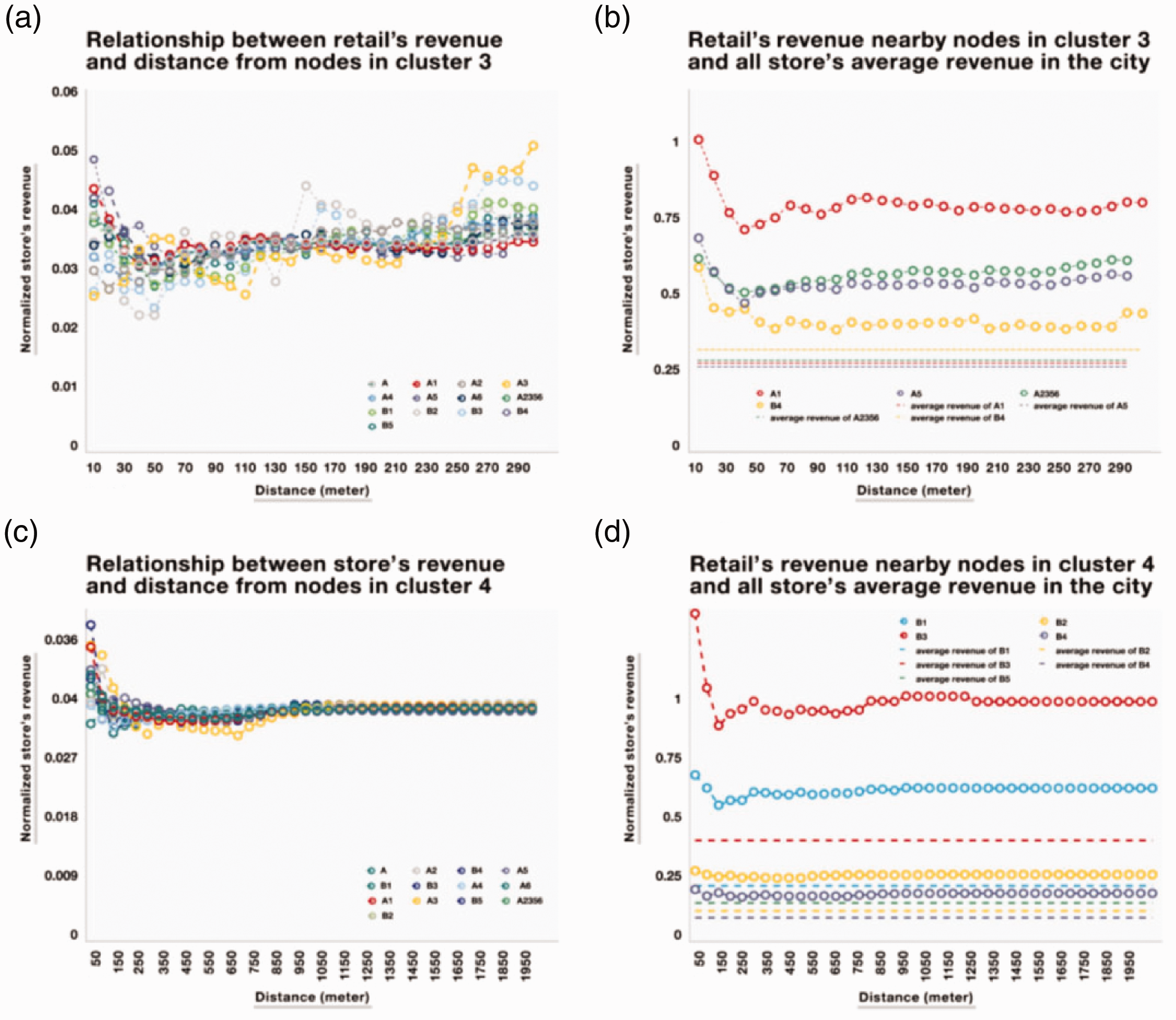
(a) The relationship between the retail store revenues in categories A and B and their distance from the nodes, which are classified into cluster 3. (b) The relationship between the retail store revenues located near nodes in cluster 3 and average store revenues in the same category (shown as flat dashed lines). (c) The relationship between the retail store revenues and their distance from the nodes, which are classified into cluster 4. (d) The relationship between the retail store revenues located near nodes in cluster 4 and the average store revenues in the same category (reported as flat dashed lines).

However, the positive effect of city-scale accessibility on retail revenue was apparent. As shown in Figure 4(c), all shop categories had a peak in normalized revenue for shorter distances to the city-scale accessible nodes; i.e. nodes belonging to cluster 4. It was also found that the revenue for the stores located near the accessible nodes at either the local (Figure 4(b)) or the city scale (Figure 4(d)) was much higher than average.

To summarize, the analysis revealed that nodes with relatively high city-scale accessibility contributed positively to store revenue; however, this effect for locally accessible nodes (cluster 3) was only observed in daily-use stores, which confirmed the intuition that these stores better capture passers-by than less locally accessible stores. Following this intuition, customers of daily-use stores (e.g. butchers and fishmongers) would be more likely to be drawn from nearby locations rather than from far away; that is, locally accessible shops are more likely to observe more customers. However, locally accessible nodes were not found to have the same effect for other categories (e.g. B2 and B3) because the customers tended to come from a much wider district or city-scale areas.

As the nodes in cluster 4 were found to increase store revenue independent of type, these nodes could be considered central places when considering larger network sizes, such as district or city scales as they more frequently captured passers-by from the whole city than other places. Therefore, these locations are advantageous for non-daily-use category stores (e.g. department stores) that derive their customers from a wider area than the local neighborhood. Although those nodes increased revenue across all categories, a further observation found that stores located at distances as far as 1 km from the nodes in cluster 4 had much higher revenues than the average revenue of all stores in the city. For example, the revenue in the category A1 stores located near the cluster 4 nodes was 3.7 times higher than the average revenue for the whole city. Surprisingly, the same tendency was found for cluster 3 nodes, where most of the environment was pedestrianized and the revenue was 3.5 times higher for category A1.

Discussion and conclusions

Based mainly on correlation analysis, this paper examined the relationships between the spatial clustering of retail stores, the transaction numbers, and the urban structure derived from the street networks in Barcelona, Spain.

Store clustering locations did not necessarily result in higher revenues, and that store density did not explain sales volume distributions, which was an intriguing result as it was not in line with the general belief that the more the retail stores in an area, the higher the expected sales volume. The exception was category A3 (personal equipment); although A3’s store density had lower $R^{2}$ scores for sales volume, its clustering locations explained the clustering of its higher revenues ( $R^{2}$ = 0.61, p < 0.01). Therefore, it was speculated that for store categories wherein the shopping is mostly intentional such as jewelry, a spatial clustering of retailers could benefit customers and store owners, as customers tend to explore nearby stores to compare items and prices before purchase. Thus, the store owner can expect a spillover of customers from nearby stores (Eaton and Lipsey, 1982), which overcomes the competition from nearby stores offering similar items. Therefore, for certain retailers, the physical proximity of other similar stores makes it possible for customers to check item quality, which reduces customer search costs (Nelson, 1970) and benefits the stores. The spatial clustering locations of A3 + B4 or B3 (personal equipment + café/restaurant) stores had higher revenue correlations, from which it was speculated that people tended to visit a café or restaurant before or after shopping in the A3 stores, which means that the store owners in both categories (e.g. A3 and B4) can obtain benefits if they are located in the same cluster.

The analysis of the relationships between location and revenue found that (1) stores located close to city-scale accessible nodes had higher than average revenues and (2) some categories of stores located close to locally accessible nodes also had higher than average revenues. This finding was consistent with previous research, wherein betweenness centrality was correlated with the distribution of the retail and services densities on the ground floor (Porta et al., 2009) and on all floors (Porta et al., 2012). However, the current paper’s analysis went a step further. While previous research focused on assessing the presence of retail stores and their distribution and have therefore speculated about the respective sales volumes (e.g. may be higher), the analysis in this paper found the location and revenue relationships based on empirical datasets. Further, secondary activities were found to be located and concentrated not only in secondary streets but also in primary streets, in line with previous research (Porta et al., 2012). However, it was discovered that the stores located near the primary and secondary streets had higher than average revenues.

The obtained results can be interpreted as follows. As daily-use stores are largely oriented toward neighborhood customers rather than the whole district or city, they could optimize location choice by considering a five-minute walking distance, which would explain why only the daily-use store revenues were higher near the cluster 3 nodes, as shown in Figure 4(a) and (b). Daily-use stores might also tend to choose in-between locations that people pass by rather than being the origin or destination as these locations enable daily-use stores to capture customers from non-daily-use stores when the latter’s customers move from origin to destination, which may also be why daily-use store revenues were found to be higher near cluster 4 nodes, as shown in Figure 4(c) and (d). However, as the non-daily-use stores are more oriented toward attracting global customers from the city scale rather than the neighborhood scale, they focus on a wider-scale network; therefore, as presented in Figure 4(c) and (d), their revenues were higher near cluster 4 nodes but not near cluster 3 nodes (Figure 4(a) and (b)).

The results also reinforced previous studies’ findings, elucidating the possible causes for spatial retail clustering. Studies have hypothesized that when customer knowledge about items and prices in each store was incomplete, they tended to search for and compare similar products and prices between stores before making a final purchase. Therefore, if several similar stores were spatially clustered, customers could reduce their search costs and retailers could expect customer spillover from other stores, which would increase the probability of attracting more customers and receiving higher sales volumes. Adding to previous findings, this study provided a statistically sound quantification of the relation between the associated variables and found that this tendency was stronger for luxury personal equipment than for daily-use goods because customers are strategic and conservative when purchasing items in luxury stores. Therefore, our study suggests that customers would be relatively more likely to browse similar luxury stores in clusters than browsing similar daily-use stores.

Although this paper’s methodology and analysis provide clear value and novel perspectives on existing research in the field, certain limitations were noted. As our study focused on providing a solid correlation analysis between various spatial variables, its scope excludes the exploration of the possible causes of such observed correlations. Regarding the analysis of possible causal relationships, we acknowledge that several possible confounding factors were not considered in this paper. For instance, looking at spatial clustering of store location, it is not clear as to what extent the process of locating a store is influenced by local planning and retail policies. This might include incentives and/or disincentives to certain types of retail activities in a certain neighborhood. One way of accounting for this and extending this study is to enrich the models through, for example, the traditional data collection methods (e.g. interviews or questionnaires and research of present and past planning and incentive policies). This way, it would be possible to start exploring causal relationships between the observed variables. Our approach can then be considered as complementary to conventional study methods (Borgman, 2015).

This paper contributes to empirical data analysis and validates previously proposed human behavior theories related to economic activities. The observed datasets are different from experimental datasets as they register human activities as is rather than limiting the external factors because of the subsequent statistical analysis. As not all human economic activities are necessarily observable, unique analytical methodologies are required to uncover the mechanisms behind the observations. Therefore, the results of this study provide quantitative and empirical verification of Jacobs’ (1961) observations.

Supplemental Material

sj-pdf-1-epb-10.1177_2399808320954210 - Supplemental material for Spatial clustering: Influence of urban street networks on retail sales volumes

Supplemental material, sj-pdf-1-epb-10.1177_2399808320954210 for Spatial clustering: Influence of urban street networks on retail sales volumes by Yuji Yoshimura, Paolo Santi, Juan Murillo Arias, Siqi Zheng and Carlo Ratti in EPB: Urban Analytics and City Science

Footnotes

Acknowledgment

We would like to thank the Banco Bilbao Vizcaya Argentaria (BBVA) for providing the dataset for this study.

Declaration of conflicting interests

The author(s) declared no potential conflicts of interest with respect to the research, authorship, and/or publication of this article.

Funding

The author(s) received no financial support for the research, authorship, and/or publication of this article.

ORCID iD

Yuji Yoshimura

Supplemental material

Supplemental material for this article is available online.

Yuji Yoshimura, architect and PhD in computer sciences, is a project associate professor at Research Center for Advanced Science and Technology, the University of Tokyo. His research focuses on urban sciences, which is the intersections of architecture, urban planning, and science.

Paolo Santi is a principal research scientist at MIT Senseable City Lab where he leads the MIT/Fraunhofer Ambient Mobility initiative and a research director at the Istituto di Informatica e Telematica, CNR, Pisa. His research interest is in modeling and analysis of complex systems ranging from wireless multi hop networks to sensor and vehicular networks.

Juan M Arias is in charge of stakeholders engagement at BBVA Data Strategy area. He has extensive experience as urban planner and project manager in technological innovation initiatives. He is part of a group of Experts that the European Commission selected to foster Business to Government Data-Sharing initiatives.

Siqi Zheng is a Samuel Tak Lee professor at the Massachusetts Institute of Technology, where she directs the Sustainable Urbanization Lab. Her research area is urban and environmental economics, and her research interests include environmental sustainability, place-based policies, and self-sustaining urban growth.

Carlo Ratti is a professor of the practice of urban technologies at the Massachusetts Institute of Technology, where he directs the SENSEable City Laboratory. He is also founding partner and director of Carlorattiassociati, an architectural firm. His research interests include urban design, human–computer interfaces, electronic media, and the design of public spaces.

References

Albert

Barabási

A-L

(2002) Statistical mechanics of complex networks. Reviews of Modern Physics 74(1): 47–97.

Alonso

(1964) Location and Land Use. Location and Land Use. Cambridge, MA: Harvard University Press.

Anselin

(1988) Spatial Econometrics: Methods and Models. Dordrecht: Kluwer Academic.

Barabási

A-L

Albert

(1999) Emergence of scaling in random networks. Science (New York, N.Y.) 286(5439): 509–512.

Barthélemy

Bordin

Berestycki

, et al. (2013) Self-organization versus top-down planning in the evolution of a city. Scientific Reports 3: 2153.

Barthélemy

Flammini

(2008) Modeling urban street patterns. Physical Review Letters 100(13): 138702.

Bohn

Andreotti

Douady

, et al. (2002) Constitutive property of the local organization of leaf venation networks. Physical Review. E, Statistical, Nonlinear, and Soft Matter Physics 65(6): 61914.

Borgman

(2015) Big Data, Little Data, No Data: Scholarship in the Networked World. Cambridge, MA: MIT Press.

Cardillo

Scellato

Latora

, et al. (2006) Structural properties of planar graphs of urban street patterns. Physical Review E 73(6): 066107.

10.

Christaller

Baskin

(1966) Central Places in Southern Germany. Englewood Cliffs, NJ: Prentice Hall.

11.

Crucitti

Latora

Porta

(2006) Centrality measures in spatial networks of urban streets. Physical Review E 73(3): 036125.

12.

DiPasquale

Wheaton

(1996) Urban Economics and Real Estate Markets. Englewood Cliffs, NJ: Prentice Hall.

13.

Eaton

Lipsey

(1982) An economic theory of Central places. The Economic Journal 92: 56–72.

14.

Fotheringham

Brundson

Chalrton

(2000) Qualitative Geography. Perspectives on Spatial Data Analysis. The Sage Handbook of Qualitative Geography. London, UK: Saga Publications.

15.

Freeman

(1977) A set of measures of centrality based on betweenness. Sociometry 40(1): 35.

16.

Fujita

Thisse

(2013) Economics of Agglomeration. Cambridge: Cambridge University Press.

17.

Getis

Ord

(1996) Local spatial statistics: An overview. In: Longley

Batty

(eds) Spatial Analysis: Modeling in a GIS Environment. New York: John Wiley & Sons, pp.261–277.

18.

Gil

(2017) Street network analysis “edge effects”: Examining the sensitivity of centrality measures to boundary conditions. Environment and Planning B: Urban Analytics and City Science 44(5): 819–836.

19.

Hillier

(1996) Space is the Machine : A Configurational Theory of Architecture. Cambridge: Cambridge University Press.

20.

Hillier

Hanson

(1984) The Social Logic of Space. Cambridge: Cambridge University Press.

21.

Huff

(1963) A probabilistic analysis of shopping center trade areas. Land Economics 39(1): 81–90.

22.

Jacobs

(1961) The Death and Life of Great American Cities. New York: Random House.

23.

Jiang

(2007) A topological pattern of urban street networks: Universality and peculiarity. Physica A: Statistical Mechanics and Its Applications 384(2): 647–655.

24.

Jiang

Claramunt

(2004) Topological analysis of urban street networks. Environment and Planning B: Planning and Design 31(1): 151–162.

25.

Jiang

Duan

, et al. (2014) Topological structure of urban street networks from the perspective of degree correlations. Environment and Planning B: Planning and Design 41(5): 813–828.

26.

Kang

Yang

Peters

, et al. (2016) Empirical analysis of road networks evolution patterns in a government-oriented development area. Environment and Planning B: Planning and Design 43(4): 698–715.

27.

Krugman

(1996) The Self Organizing Economy. New Jersey: Wiley-Blackwell.

28.

Lämmer

Gehlsen

Helbing

(2006) Scaling laws in the spatial structure of urban road networks. Physica A: Statistical Mechanics and Its Applications 363(1): 89–95.

29.

Lösch

(1954) The Economics of Location. New Haven, CT: Yale University Press.

30.

Lucas

(1988) On the mechanics of economic development. Journal of Monetary Economics 22(1): 3–42.

31.

Omer

Osaragi

, et al. (2019) Why topology matters in predicting human activities. Environment and Planning B: Urban Analytics and City Science 46(7): 1297–1313.

32.

March

Steadman

(1971) The Geometry of Environment. An Introduction to Spatial Organization in Design. London, UK: RIBA.

33.

Martin

March

(1972) Urban Space and Structures. Cambridge, UK: Cambridge University Press.

34.

Masucci

Stanilov

Batty

(2014) Exploring the evolution of London’s street network in the information space: A dual approach. Physical Review E 89(1): 1–7.

35.

Mills

(1967) An aggregative model of resource allocation in a metropolitan area. The American Economic Review 57(2): 197–210.

36.

Mitchell

(2009) The ESRI Guide to GIS Analysis, Volume 2: Spatial Measurements and Statistics. Redlands, CA: Esri Press.

37.

Muth

(1969) Cities and Housing. Chicago, IL: University of Chicago Press.

38.

Nelson

(1970) Information and consumer behavior. Journal of Political Economy 78(2): 311–329.

39.

Okabe

Sugihara

(2012) Spatial Analysis along Networks: Statistical and Computational Methods. West Sussex, UK: John Wiley & Sons.

40.

Ord

Getis

(1995) Local spatial autocorrelation statistics: Distributional issues and an application. Geographical Analysis 27(4): 286–306.

41.

Perna

Kuntz

Douady

(2011) Characterization of spatial networklike patterns from junction geometry. Physical Review E 83(6): 57–59.

42.

Porta

Crucitti

Latora

(2006a) The network analysis of urban streets: A dual approach. Physica A: Statistical Mechanics and Its Applications 369(2): 853–866.

43.

Porta

Crucitti

Latora

(2006b) The network analysis of urban streets: A primal approach. Environment and Planning B: Planning and Design 33(5): 705–725.

44.

Porta

Latora

Wang

, et al. (2012) Street centrality and the location of economic activities in Barcelona. Urban Studies 49(7): 1471–1488.

45.

Porta

Strano

Iacoviello

, et al. (2009) Street centrality and densities of retail and services in bologna. Environment and Planning B: Planning and Design 36(3): 450–465.

46.

Sevtsuk

(2010) Path and place: A study of urban geometry and retail activity in Cambridge and Somerville, MA. PhD Dissertation, MIT Department of Urban Studies and Planning, Cambridge, MA.

47.

Sevtsuk

(2014) Location and agglomeration: The distribution of retail and food businesses in dense urban environments. Journal of Planning Education and Research 34(4): 374–393.

48.

Strano

Viana

Costa

LdF

, et al. (2013) Urban street networks, a comparative analysis of ten European cities. Environment and Planning B: Planning and Design 40(6): 1071–1086.

49.

Tobler

(1970) A computer movie simulating urban growth in the Detroit region. Economic Geography 46: 234.

50.

Von Thünen

(1826) The Isolated State. Oxford, UK: Pergamon Press.

51.

Watts

Strogatz

(1998) Collective dynamics of ‘small-world’ networks. Nature 393(6684): 440–442.

52.

Yoshimura

Sobolevsky

Bautista Hobin

, et al. (2018) Urban association rules: Uncovering linked trips for shopping behavior. Environment and Planning B: Urban Analytics and City Science 45(2): 367–385.

Supplementary Material

Please find the following supplemental material available below.

For Open Access articles published under a Creative Commons License, all supplemental material carries the same license as the article it is associated with.

For non-Open Access articles published, all supplemental material carries a non-exclusive license, and permission requests for re-use of supplemental material or any part of supplemental material shall be sent directly to the copyright owner as specified in the copyright notice associated with the article.

0.00 MB

0.34 MB