A two-dimensional propensity score matching method for longitudinal quasi-experimental studies: A focus on travel behavior and the built environment

Abstract

The lack of longitudinal studies of the relationship between the built environment and travel behavior has been widely discussed in the literature. This paper discusses how standard propensity score matching estimators can be extended to enable such studies by pairing observations across two dimensions: longitudinal and cross-sectional. Researchers mimic randomized controlled trials and match observations in both dimensions to find synthetic control groups that are similar to the treatment group and to match subjects across before- and after-treatment periods. We call this a two-dimensional propensity score matching method. This method demonstrates superior performance for improving treatment effect estimation based on Monte Carlo evidence. A near-term opportunity for such matching is identifying the treatment effect of transportation infrastructure on travel behavior.

Keywords

Built environment travel behavior causal inference propensity score matching

Introduction

Despite the growing empirical evidence on the association between travel behavior and the built environment, there remains the need for the causal understanding of the relationship between the built environment and travel behavior (Guan et al., 2020; Heinen et al., 2018; Mokhtarian and Cao, 2008). In order to draw causal inferences, under the potential outcome framework, we need experimental data that have a randomized assignment to treatment and observe the same groups of individuals before and after the treatment (Lewis, 1973; Rubin, 1974, 2005). However, built environment research, as in all observational studies, faces multiple challenges for causal inferences, namely the cross-sectional and self-selected samples and the nonrandom assignment of treatments. As true experiments are mostly infeasible, researchers use natural experiments that rely on quasi-random assignment to estimate treatment effects. Among the various econometric methods, matching has been widely used to address the selection bias in nonexperimental studies (Thoemmes and Kim, 2011) and the residential self-selection bias (Cao, 2010; Cao and Fan, 2012; Cao et al., 2010; Mokhtarian and van Herick, 2016).¹

However, the strength of matching methods in previous studies is hampered by the lack of time precedence between changes in the built environment and travel behavior (Mokhtarian and Cao, 2008).² Because panel data are scarce, researchers can only apply matching to cross-sectional data. By contrast, repeated cross-sectional (RCS) data are abundant, including the National Household Travel Survey, the American Community Survey, and travel surveys conducted by Metropolitan Planning Organizations. These RCS data observe the set of individuals that may not be identical over time, but they have theoretical support for constructing quasi-experiments and estimating aggregate-level effects (Kramer, 1983). The aggregate-level effects, in this case, the behavioral changes at the neighborhood level, are of interest to evaluation questions about transportation and land use interventions.

With this perspective, we aim to develop a matching method that can be used for constructing pseudo-panel data from the abundant RCS data. In order to do so, we need to address two biases in RCS data.

First, selection bias: selection bias occurs when the estimated samples are nonrandomly assigned to a treatment group and a control group because of self-selection.

Second, longitudinal incomparability: this bias occurs when the estimated samples may be systematically different before and after the intervention because there are no true panel data.

We propose a two-dimensional propensity score matching (2DPSM) method as a tool to pair individuals between the treated and control groups on both the longitudinal and cross-sectional dimensions based on their characteristics. Therefore, using 2DPSM, a longitudinal quasi-experimental setting is constructed by mimicking a random assignment on the cross-sectional dimension and pairing statistically identical individuals over time.

This method has several advantages. First, it enables researchers to construct quasi-longitudinal data using widely available RCS survey data cost-effectively. For example, the 2DPSM method has the potential to longitudinally match respondents from two separate travel surveys for the same region that take place a few years apart. Researchers can use this method to construct a quasi-experimental setting based on respondents from the two surveys when true experiments are not feasible.

Second, it improves causal interpretation by matching individuals at both cross-sectional and longitudinal dimensions under the selection on observables assumption. Previous studies have used matching to improve the estimation of treatment effects but lack a causal interpretation in the absence of longitudinal dimension matching. Even when the selection on observables assumption does not hold, our Monte Carlo evidence also shows that 2DPSM produces more accurate results than one-dimensional (1D) matching.

The rest of the paper is organized as follows. The upcoming section illustrates the 2DPSM framework and introduces the protocol of applying 2DPSM. Next section reports simulation results that explore the performance of 2DPSM under scenarios with and without unobserved variables and compares it with 1D matching. The last section concludes and offers application guidelines.

Two-dimensional propensity score matching

Biases in quantities of interest

To illustrate the 2DPSM framework, we briefly describe a typical example of travel behavior and the built environment research. Consider a public transit system opening in the neighborhood as the treatment, individuals within the impact zone (typically 0.5 mile) of public transit stations as being treated, and ridership as the outcome. In general, policymakers and researchers are interested in the effects of such transit station openings on residents and local businesses. Of course, such an effect can be dynamic, heterogeneous, and nonlinear, depending on contexts and time (Chatman, 2014). Here, we focus on the average treatment effect (ATE), with a focus on individual behaviors. In a typical setting, we have four groups of people related to the opening of a new transit system: (1) before the opening and within the impact zone (before and potentially treated [BT]), (2) before the opening and beyond the impact zone (before and control [BC]), (3) after the opening and within the impact zone (after and treated [AT]), and (4) after the opening of the transit system and beyond the impact zone (after and control [AC]), as represented in Figure 1.

Figure 1.

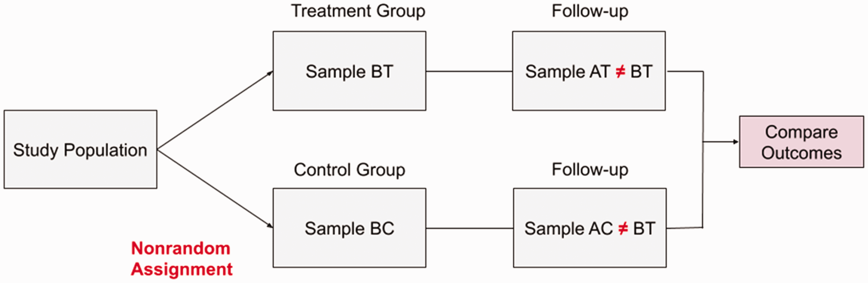
A typical setting of travel behavior and the built environment research.

Suppose we have individuals i (i = 1 to n) and their associated travel behaviors at time t taking the new public transit if living nearby transition stations [represented by Y _it (1)] and if living beyond station areas [represented by Y _it (0)]. The treatment effect (TE) on an individual is defined as Y _it (1) − Y _it (0). First, we assume that Y _it is given by a linear factor model

Y_{i t} = δ_{i t} T_{i t} + x_{i t}^{'} β + λ_{i}^{'} f_{t} + ε_{i t}

(1)

where the treatment indicator T _it equals 1 if individual i has been exposed to the treatment prior to time t and equals 0 if not and

δ_{i t}

is the heterogeneous treatment effect on individual i at time t. In this paper, for simplicity, we focus on ATT, which is the ATE on treated individuals in the sample.³ Given our earlier discussion on ideal RCTs, the standard difference-in-differences (DID) estimator can be written as

SATT = E [Y_{i t 1} (1) - Y_{i t 1} (0)] - E {[Y}_{i t 0} (1) - Y_{i t 0} (0)]

(2)

Time periods t₁ and t₀ denote before and after treatment, respectively. In reality, one individual can be in only the control group or the treatment group. Therefore, we can observe only one outcome for the individual i: Y_i(1) or Y _i (0). In the treatment group, Y_i(1) is observed and Y _i (0) is unobservable. Y _i (0) will be replaced by the outcome Y _j (0) of a matched subject j from the control group; this is where selection bias may arise. Moreover, because individuals are not tracked over time in RCS data, compositions of the treatment group and the control group are likely to be different after interventions; this is where longitudinal incomparability may arise.

Two-dimensional propensity score matching framework

Two-dimensional propensity score matching is proposed to mimic a quasi-experimental situation wherein the four groups of individuals are conditionally exchangeable (see Figure 2). The two main sources of estimation bias are selection bias, in which individuals with certain characteristics self-select to the treatment group, and longitudinal incomparability, in which individuals may not be in the same groups of people after the intervention. On the cross-sectional dimension, we match individuals with similar propensity scores, which is the probability of being in the treatment group based on their characteristics. On the longitudinal dimension, we match individuals with statistically identical characteristics. The matchings on both the cross-sectional and longitudinal dimensions are expected to reduce the estimation bias that results from self-selection and incomparability.

Figure 2.

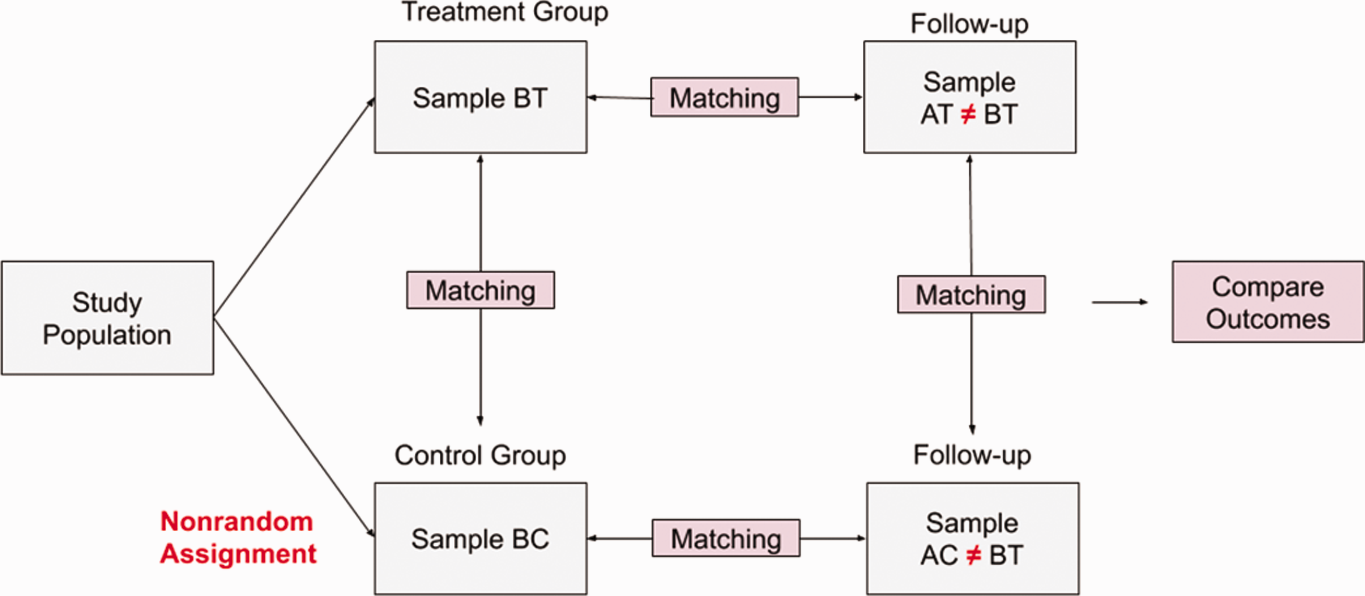
Proposed two-dimensional propensity score matching for causal inference.

Matching plays the central role of summarizing all the relevant information and balancing the set of observed covariates across groups. After matching on both the longitudinal and cross-sectional dimensions, equation (2) can be rewritten as

D_{0} = E [Y_{i t 0 matched} (1) - Y_{j t 0 matched} (0)| m (X_{a}^{b}), m (X_{c}^{t})] and

(3)

D_{1} = E [Y_{i t 1 matched} (1) - Y_{j t 1 matched} (0)| m (X_{a}^{b}), m (X_{c}^{t})] such that

(4)

SATT = {(D}_{1} - D_{0}) | X

(5)

D₀ and D₁ are the differences in means between the treatment and control groups before and after treatment, respectively. m( $X_{a}^{b}$ ) and m( $X_{c}^{t}$ ) denote matching on the cross-sectional (before treatment [b] and after treatment [a]) and longitudinal dimensions (before and after treatment groups [t] and before and after control groups [c]). When matching is properly applied to both dimensions, the before- and after-treatment and treatment–control groups are balanced with similar distributions of covariates. Hypothetically, the difference between D₁ and D₀ is defined as SATT over the common support of X. The underlying assumption is that the common support among the four groups must be met. In travel behavior research, in most cases, the subjects grouped by geographical areas and temporal periods are not dramatically different. The application of this framework also requires the usual selection on observables assumption, in which the selection or assignment of the before- and after-treatment and treatment–control groups depends only on the observed characteristics of the individuals (Rubin, 1977).

Matching protocol

In this section, we describe the matching protocol for 2DPSM. On the cross-sectional dimension, propensity score matching (PSM) is used for matching, because selection bias is essentially the unequal probability of a subject being assigned to treatment and control groups. On the longitudinal dimension, we use either PSM or Mahalanobis distance matching (MDM) to minimize the differences in observed characteristics of individuals.

2DPSM Framework: A matching procedure that sequentially pairs individuals in each before- and after-treatment group and treatment–control group and takes the following steps:

Step 1. Start the first round of matching for each group.

(a) Start matching individuals in BT with individuals in AT.

(b) Use matched individuals in BT to match with individuals in BC.

(d) Use matched individuals in AT to match with matched individuals in AC.

End of this step. Matched individuals in each group are collected.

Step 2. Start a loop that runs R times:

(a) In round 1, repeat the procedure in step 1 with matched individuals.

(b) Continue to round 2 if the numbers of matched individuals in each group are not equal. Otherwise, end the loop and collect matched individuals in each group.

(d) Continue the loop if the numbers of matched individuals in each group are not equal. Otherwise, end the loop and collect matched individuals in each group.

(e) Break the loop if the numbers of individuals are out of range due to pruning during the matching process. No matched individuals can be collected.

End of the loop.

Step 3. Check the imbalance of the covariates.

For the cross-sectional dimension, check imbalance for BT:BC and AT:AC.

For the longitudinal dimension, check imbalance for BT:AT and BC:AC.

Matching on the longitudinal and cross-sectional dimensions could involve several methods that can balance covariates’ distributions in treatment and control groups, including optimal matching and greedy nearest neighbor matching (NNM) (Guo and Fraser, 2014). Optimal matching pairs subjects to minimize the average within-pair differences in propensity score for the whole groups. In contrast, in greedy NNM, a treated subject is selected and then paired with an untreated subject with a propensity score closest to that of the treated subject. Also, greedy NNM has several varieties that differ based on whether subjects are removed during the matching process (i.e. with or without replacement), whether matched pairs beyond a chosen caliper are removed (caliper matching), and whether one subject is matched to another or to many others (one-to-one or many-to-one matching). We develop and evaluate 2DPSM based on regression-based methods, but researchers can use more advanced methods, such as machine learning algorithms, under this protocol.

Evaluating the performance of 2DPSM

In this section, we conduct Monte Carlo exercises to explore the performance of 2DPSM and compare it with one-dimensional propensity score matching under different scenarios, including varying levels of imbalance and different prevalence of treatment. We also investigate the extent to which 2DPSM can relax the selection on observables assumption. Because the true treatment effects are unknown within any real-world travel data or any nonrandomized data, we need simulation-based research to evaluate the performance of 2DPSM.

Data generation process

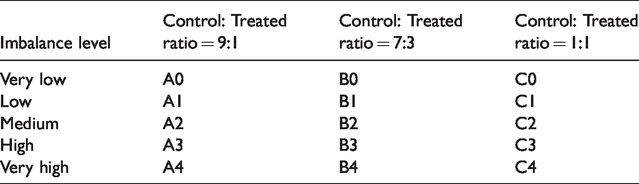
We start with a data generating process (DGP) that is similar to Gu and Rosenbaum (1993) and King and Nielsen (2016). The DGP includes four observed variables and one error term. Four covariates (X1, X2, X3, X4) are drawn from a normal distribution with variances of 1 and covariances of 0.2 and 0.9. We set the control group mean vector to (0, 0, 0, 0) and treatment group mean vector before treatment to (0.1, 0.1, 0.1, 0.1). After treatment, we set the treatment group mean vector to (0.1, 0.1, 0.1, 0.1), (0.3, 0.3, 0.3, 0.3), (0.5, 0.5, 0.5, 0.5), (1, 1, 1, 1), and (2, 2, 2, 2) to represent very low, low, medium, high, and very high imbalance levels, respectively. For each level of imbalance, we generate a pool of 1,000,000 observations and create 1000 data sets by sampling 1,000 observations from the pool each time. In each data set, the control: treatment ratio is determined by the number of treatment observations (100, 300, or 500). The treatment effect is set to be 0.6, which means that the treated individuals are more likely to change their travel behaviors (e.g. on average, increase 0.6 daily walking trips) than the control individuals. The coefficients of the four covariates take the following values based on Austin (2011): low effect log (1.25), medium effect log (1.5), high effect log (1.75), and very high effect log (2). The error term is randomly drawn from the normal distribution, which has a variance of 0.5 and a mean of 0. Together, the five imbalance levels and the three ratios of control subjects to treated subjects defined 15 scenarios, which are summarized in Table 1.

Table 1.

Simulation settings by imbalance level and Control: Treated ratio.

Imbalance level	Control: Treated ratio = 9:1	Control: Treated ratio = 7:3	Control: Treated ratio = 1:1
Very low	A0	B0	C0
Low	A1	B1	C1
Medium	A2	B2	C2
High	A3	B3	C3
Very high	A4	B4	C4

Matching scenarios

We then test the performance of various specifications of 2DPSM on the simulated samples. We specify both PSM and MDM without replacement. Thus, a treated subject is randomly selected and paired with an untreated subject whose propensity score is closest to that of the selected subject. Once an untreated subject is matched with a treated subject, the untreated subject is removed from the pool and will not be further considered in the matching process. To define the closeness, we use the two caliper values: 0.2 SD and 1 SD of the average propensity score.⁴

For comparison, we also report two other methods: (1) estimation without matching and (2) a common practice in the literature in which individuals are matched only on the cross-sectional dimension. We report each method and specifications of 2DPSM in Table 2.

Table 2.

Matching scenarios and 2DPSM specifications.

Matching scheme	Notation	Description
No matching	Naïve	No matching is implemented.
One-dimensional propensity score matching	1D	PSM is implemented on the cross-sectional dimension (caliper 0.2 × SD); covariates are included for longitudinal comparison.
Two-dimensional propensity score matching	2D-1	PSM is implemented on the cross-sectional dimension (caliper 1 × SD), and MDM is implemented on the longitudinal dimension.
	2D-2	PSM is implemented on both the cross-sectional and longitudinal dimensions (caliper 0.2 × SD).
	2D-3	PSM is implemented on both the cross-sectional and longitudinal dimensions (caliper 1 × SD).

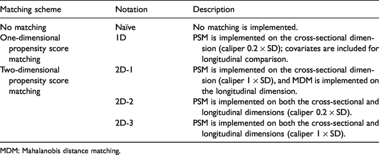
MDM: Mahalanobis distance matching.

Checking imbalance

We rely on the standard difference to measure the imbalance between the treated and matched controls (d’Agostino, 1998). The standardized difference is calculated as

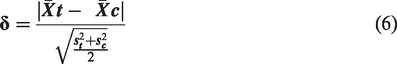
δ = \frac{|\bar{X} t - \bar{X} c|}{\sqrt{\frac{s_{t}^{2} + s_{c}^{2}}{2}}}

(6)

The conventional indicator of balance is a standardized difference $δ \leq 10 %$ between treatment and control groups (Oakes and Johnson, 2006). Each matching scheme is applied to 1000 simulated samples. We check the imbalance between the treatment group after treatment and other groups. The imbalances of X1 and X2 without matching range from 0.1 to 2 between the treatment group after treatment and other groups; the other groups initially all had a high balance. After matching, all 2DPSM specifications reduce a significant degree of imbalance between the treatment group after treatment and other groups. The 1D specification fails to reduce the longitudinal imbalance that may or may not be accommodated by regression analysis. Among all the specifications, in most cases, 2D-2, which has a smaller caliper, resulted in the most substantial reductions in the imbalance. See Supplemental Figures S1 to S4 for a detailed imbalance check.

Measuring performance

After matching, we examine the performance of each matching scheme in improving the estimation of the DID estimator. In order to evaluate the performance of 2DSPM, we directly estimate the matched sample without controlling for observed variables. We use six criteria to assess the performance:

Matched sample size: matched sample size is the final sample size after matching because a small matched sample size can inflate the variance of the treatment effect.

Estimated treatment effect: point estimates of treatment effects.

Standard deviation: the standard deviation of the estimated treatment effect.

Absolute bias ratio: the ratio of difference from the true treatment effect.

Root mean square error: the square root of the average squared differences between the estimated treatment effect and the true treatment effect.

95% confidence interval (CI) coverage: the percentage of the estimated treatment effects that fall within the 95% CI of the true treatment effect.

Figure 3 presents the performance metrics of the various matching schemes specified in Table 2. Supplemental Table S1 reports the numerical values of the performance metrics. First, we find that 1D has slightly better performance across all scenarios but does not qualitatively differ from 2D-1, 2D-2, and 2D-3. Second, although 2D-1 has relatively better performance than 2D-2 and 2D-3, it drops too many observables when matching samples with higher imbalance levels. This issue is likely because MDM does not work well when there are relatively many variables, as it tries to match more of the multiway interactions among the variables. Finally, 2D-2 and 2D-3 can be applied in a broader range of imbalance levels and prevalence than 2D-1. Supplemental Table S2 documents that 2D-1 is not feasible unless the imbalance level is low. However, with increasing imbalance level, 2D-2 performs better than 2D-3. It is worth emphasizing that these results are under the selection on observables assumption. In the next section, we explore the sensitivity of the results to the existence of unobserved variables.

Figure 3

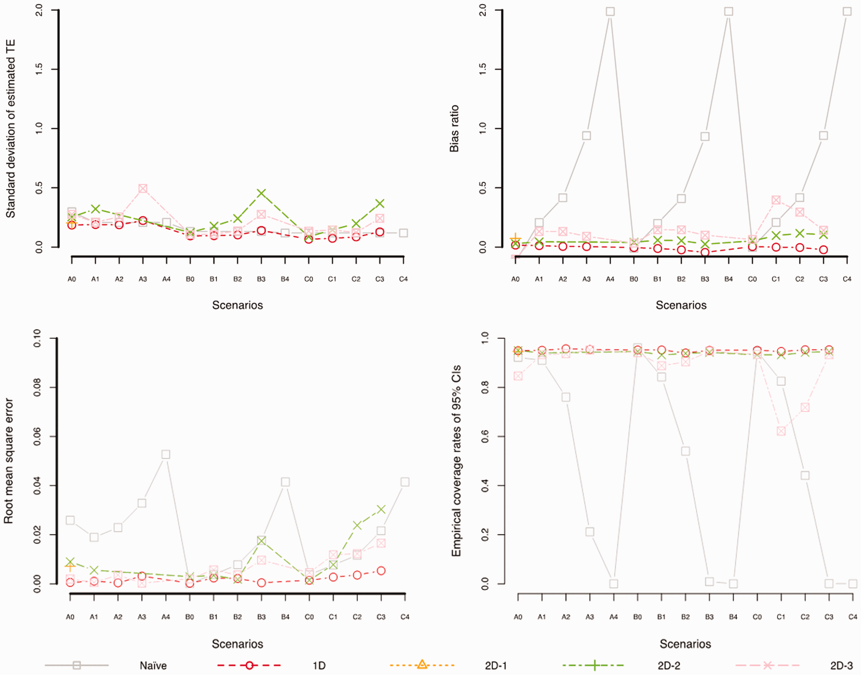
Performance metrics of matching schemes.

Sensitivity to selection on observables

In this section, we evaluate the performance of each matching scheme when the assumption of selection on observables does not hold. We modified the data generating process described in Section 5.1 to generate three scenarios:

Scenario A: no unobserved variables

Scenario B: unobserved variables are not correlated with observed variables

Scenario C: unobserved variables are either independent from or correlated with observed variables.

Among them, Scenario B is the same as the data generating process described in the Data Generating Process section, which has a random term that is independent of observed variables and follows a normal distribution with a mean of 0 and a variance of 0.5. Scenario A removes the random term from the data generating process. Scenario C, which is more aligned with the real-world data, has unobserved variables that are either correlated with or unrelated to observed variables. In this context, for a variable to be unobserved, it is included in the true data generating process but not included in matching and estimation.

Table 3 reports the results. In scenarios A and B, there is no qualitative difference in performance among 1D, 2D-2, and 2D-3. Yet, 1D and 2D-2 are slightly more stable than 2D-3. In scenario C, 2D-2 and 2D-3 have notably better 95% CI coverage than 1D, where 1D has a generally unacceptable coverage. The results suggest that 2D-2 and 2D-3 tend to outperform 1D when unobserved variables are a potential threat to the estimation. This finding is not surprising. Because matching on observed variables also matches on unobserved variables, as they are correlated with those observed variables. In contrast, the only unobserved variables of concern are those not correlated with observed variables.

Table 3.

Performance metrics of matching schemes: including unobserved variables.

		Scenario
Matching scheme	Metric	A	B	C
Naïve	Estimated TE	0.724	0.850	1.164
	Absolute bias (%)	20.6	41.6	94.0
	Standard error	0.208	0.208	0.208
	95% CI coverage (%)	91.0	76.0	21.2
1D	Estimated TE	0.521	0.535	0.300
	Absolute bias (%)	13.1	10.8	50.0
	Standard error	0.157	0.199	0.286
	95% CI coverage (%)	92.5	94.3	80.5
2D-2	Estimated TE	0.767	0.516	0.762
	Absolute bias (%)	27.8	14.0	26.9
	Standard error	0.291	0.244	0.486
	95% CI coverage (%)	90.7	93.6	93.7
2D-3	Estimated TE	0.617	0.451	0.536
	Absolute bias (%)	28.0	24.8	10.6
	Standard error	0.178	0.217	0.3
	95% CI coverage (%)	94.6	89.3	95.1

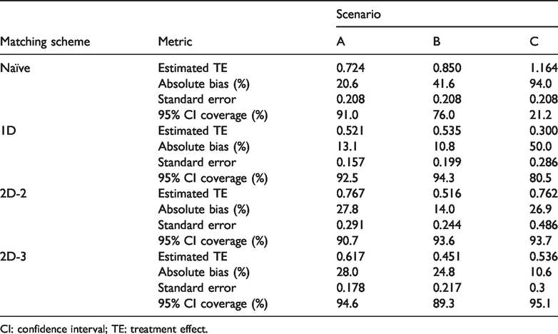
CI: confidence interval; TE: treatment effect.

Conclusion and application guidelines

Conclusion

Repeated measurements over time of residents’ travel behavior, such as the National Household Travel Survey, the American Community Survey, and travel surveys conducted by Metropolitan Planning Organizations, are underutilized for quasi-experimental design in travel behavior and the built environment research due to the lack of econometric tools. In this paper, we propose a new framework of applying matching methods on the longitudinal and cross-sectional dimensions that establish pseudo-panel data from repeated cross-sections. It attempts to address data and causal inference barriers in the study of travel behavior and the built environment; specifically, 2DPSM pairs individuals with similar characteristics from each of the before- and after-treatment and treatment–control groups.

This method is in the spirit of original matching methods in that it pairs statistically identical individuals from the treatment and control groups in order to ensure the balance of the covariates between those groups. It improves the original matching methods in two ways. First, it offers a framework that reduces selection bias and improves longitudinal comparability. Second, it allows different matching algorithms to be implemented under this framework.

Using Monte Carlo evidence, we demonstrate that 2DPSM has advantages over the common practice of matching: (1) it produces comparable estimates to that of 1D matching but offer a causal interpretation under the selection on observables assumption; (2) it produces more accurate and reliable estimates than 1D matching when the selection on observables assumption does not hold. One caveat, which is also emphasized elsewhere (Dehejia and Wahba, 2002; Ho et al., 2007; Smith and Todd, 2001), is that matching should be viewed as a nonparametric preprocessing tool that complements the parametric analysis techniques.

Finally, in this study, we only use the off-the-shelf versions of each of the matching algorithms so that transportation and planning researchers can easily incorporate 2DPSM into their toolbox. It is likely that 2DPSM can perform even better by integrating more advanced matching algorithms. A valuable direction for future work would be to compare whether machine learning can outperform the propensity score algorithm under our proposed 2D framework.

Application guidelines

Applying the 2DPSM requires researchers to make a few decisions. To make reasonable decisions, we need to understand the strengths and weaknesses of different specifications, which is essentially the trade-off between estimation efficiency and bias. The implementation of 2DPSM should follow the conventional PSM practice but with more attention to the extra complexity.

Then, one question arises when implementing 2DPSM: which 2DPSM specification to choose? We recommend 2D-1 as the first choice. In the 2D-1 specification, matching is conducted across both the longitudinal and cross-sectional dimensions, which is beneficial in terms of self-selection bias reduction and comparability over time. Sometimes there may be few subjects remaining during the matching process in this specification when the MDM algorithm is used on the longitudinal dimension, particularly when matching with rich information (i.e. many variables included). Under this condition, we recommend using the 2D-2 or 2D-3 specification.

If there is not sufficient overlap in the same group before and after treatment, we recommend the 1D specification to avoid forcibly matching subjects that are substantially different in terms of the estimated propensity score. This specification can reduce the self-selection bias but requires parametric techniques to control for covariates and offers no causal interpretation. No matter which specification is used, imbalance checking after matching is important so that researchers can get a better understanding of the extent to which the treatment and control groups are comparable and, therefore, of how sensitive estimates will be to the post-analysis model specifications.

Supplemental Material

sj-pdf-1-epb-10.1177_2399808320982305 - Supplemental material for A two-dimensional propensity score matching method for longitudinal quasi-experimental studies: A focus on travel behavior and the built environment

Supplemental material, sj-pdf-1-epb-10.1177_2399808320982305 for A two-dimensional propensity score matching method for longitudinal quasi-experimental studies: A focus on travel behavior and the built environment by Haotian Zhong, Wei Li Marlon G Boarnet in EPB: Urban Analytics and City Science

Footnotes

Acknowledgement

The authors received valuable comments and suggestions from various colleagues through the American Collegiate Schools of Planning (ACSP).

Declaration of conflicting interests

The author(s) declared no potential conflicts of interest with respect to the research, authorship, and/or publication of this article.

Funding

The author(s) disclosed receipt of the following financial support for the research, authorship, and/or publication of this article: This study was funded by the National Science Foundation (Award #: 1461766).

ORCID iD

Haotian Zhong

Notes

Supplemental material

Supplemental material for this article is available online.

Haotian Zhong is an Assistant Professor of urban science and planning in the School of Public Administration and Policy, Renmin University of China, China. His research examines the spatial and social implications of technological changes for cities and urban life.

Wei Li is an Associate Professor of urban planning in the Department of Landscape Architecture and Urban Planning, Texas A&M University, USA. He is committed to research, education, and service activities that lead to smart solutions for challenges faced by underserved communities and underprivileged populations.

Marlon G Boarnet is Professor of Public Policy and Chair of the Urban Planning & Spatial Analysis Department, is a renowned authority on urban economics, urban growth patterns, transportation, and regional science. He is an expert in transportation and land use, and has served on the National Research Council committee that authored “Driving and the Built Environment.

References

Austin

(2011) Optimal caliper widths for propensity-score matching when estimating differences in means and differences in proportions in observational studies. Pharmaceutical Statistics 10(2): 150–161.

Boarnet

Hong

Lee

, et al. (2013) The Exposition light rail line study: A before and after study of the impact of new light rail transit service.

Cao

(2010) Exploring causal effects of neighborhood type on walking behavior using stratification on the propensity score. Environment and Planning A: Economy and Space 42(2): 487–504.

Cao

Fan

(2012) Exploring the influences of density on travel behavior using propensity score matching. Environment and Planning B: Planning and Design 39(3): 459.

Cao

Fan

(2010) Exploring the connections among residential location, self-selection, and driving: Propensity score matching with multiple treatments. Transportation Research Part A: Policy and Practice 44(10): 797–805.

Chatman

(2014) Estimating the effect of land use and transportation planning on travel patterns: Three problems in controlling for residential self-selection. Journal of Transport and Land Use 7(3): 47–56.

d’Agostino

(1998) Tutorial in biostatistics: Propensity score methods for bias reduction in the comparison of a treatment to a non-randomized control group. Statistics in Medicine 17(19): 2265–2281.

Dehejia

Wahba

(2002) Propensity score-matching methods for nonexperimental causal studies. Review of Economics and Statistics 84(1): 151–161.

Rosenbaum

(1993) Comparison of multivariate matching methods: Structures, distances, and algorithms. Journal of Computational and Graphical Statistics 2(4): 405–420.

10.

Guan

Wang

Jason Cao

(2020) The role of residential self-selection in land use-travel research: a review of recent findings. Transport Reviews 40(3): 267–287.

11.

Guo

Fraser

(2014) Propensity Score Analysis: Statistical Methods and Applications. London: Sage Publications.

12.

Heinen

Mackett

van Wee

, et al. (2018) Residential self-selection in quasi-experimental and natural experimental studies. Journal of Transport and Land Use 11(1): 939–959.

13.

Imai

King

, et al. (2007) Matching as nonparametric preprocessing for reducing model dependence in parametric causal inference. Political Analysis 15(3): 199–236.

14.

King

Nielsen

(2016) Why propensity scores should not be used for matching. Copy at http://j. mp/1sexgVw Download Citation BibTex Tagged XML Download Paper, 378.

15.

Kramer

(1983) The ecological fallacy revisited: Aggregate-versus individual-level findings on economics and elections, and sociotropic voting. The American Political Science Review 77: 92–111.

16.

Lewis

(1973) Counterfactuals, Library of Philosophy and Logic. Oxford: Basil Blackwell.

17.

Mokhtarian

Cao

(2008) Examining the impacts of residential self-selection on travel behavior: a focus on methodologies. Transportation Research Part B: Methodological 42(3): 204–228.

18.

Mokhtarian

van Herick

(2016) Quantifying residential self-selection effects: A review of methods and findings from applications of propensity score and sample selection approaches. Journal of Transport and Land Use 9(1): 9–28.

19.

Oakes

Johnson

(2006) Propensity score matching for social epidemiology. Methods in Social Epidemiology 1: 370–393.

20.

Rosenbaum

Rubin

(1985) Constructing a control group using multivariate matched sampling methods that incorporate the propensity score. The American Statistician 39(1): 33–38.

21.

Rubin

(1974) Estimating causal effects of treatments in randomized and nonrandomized studies. Journal of Educational Psychology 66(5): 688.

22.

Rubin

(1977) Assignment to treatment group on the basis of a covariate. Journal of Educational Statistics 2(1): 1–26.

23.

Rubin

(2005) Causal inference using potential outcomes: Design, modeling, decisions. Journal of the American Statistical Association 100(469): 322–331.

24.

Smith

Todd

(2001) Reconciling conflicting evidence on the performance of propensity-score matching methods. American Economic Review 91(2): 112–118.

25.

Spears

Boarnet

Houston

(2016) Driving reduction after the introduction of light rail transit: Evidence from an experimental-control group evaluation of the Los Angeles Expo Line. Urban Studies 0042098016657261.

26.

Thoemmes

Kim

(2011) A systematic review of propensity score methods in the social sciences. Multivariate Behavioral Research 46(1): 90–118.

27.

Wang

Lin

(2019) Built environment, travel behavior, and residential self-selection: A study based on panel data from Beijing. Transportation 46(1): 51–74.

Supplementary Material

Please find the following supplemental material available below.

For Open Access articles published under a Creative Commons License, all supplemental material carries the same license as the article it is associated with.

For non-Open Access articles published, all supplemental material carries a non-exclusive license, and permission requests for re-use of supplemental material or any part of supplemental material shall be sent directly to the copyright owner as specified in the copyright notice associated with the article.

0.00 MB

0.59 MB