Multilevel Modeling of Social Segregation

Abstract

The traditional approach to measuring segregation is based upon descriptive, non-model-based indices. A recently proposed alternative is multilevel modeling. The authors further develop the argument for a multilevel modeling approach by first describing and expanding upon its notable advantages, which include an ability to model segregation at a number of scales simultaneously. The authors then propose a major extension to this approach by introducing a simple simulation method that allows traditional descriptive indices to be reformulated within a modeling framework. The multilevel approach and the simulation method are illustrated with an application that models recent social segregation among schools in London, UK.

Keywords

binomial response model hierarchical linear models multilevel models segregation indices social segregation

1. Introduction

Studies of segregation have a long history in social science research (e.g., Duncan & Duncan, 1955; Wright, 1937). In the United States, there has been great interest in measuring residential spatial segregation, particularly in relation to race and ethnicity (Massey & Denton, 1993; Taeuber & Taeuber, 1965). Research has focused on establishing how levels of segregation vary across areas and time. Typically, indices of segregation are calculated for individual cities for a series of years where each index score summarizes the variation, for example, in the observed proportion of Black individuals among the neighborhoods in each city. Once calculated, these scores can be compared in order to describe changing patterns of segregation.

Studies of segregation are also frequently carried out in education research, again in relation to race and ethnic segregation, but this time among schools (Clotfelter, 1999; James & Taeuber, 1985; Zoloth, 1976) or universities. However, segregation studies are not limited to race and ethnicity; many other types of segregation including educational, occupational, and social segregation have also been explored. For example, recent UK education research has focused on measuring changing patterns of social segregation among schools with respect to student poverty (see Allen & Vignoles, 2007, for a summary).

A wide range of indices have been proposed for measuring segregation and there is a long and considerable debate over their ideal properties (Hutchens, 2004; James & Taeuber, 1985; Massey & Denton, 1988; Reardon & Firebaugh, 2002; Taeuber & Taeuber, 1965; White, 1986; and Zoloth, 1976). Indeed, as Jahn, Schmid, and Schrag (1947) point out, there is virtually no limit to the number and variety of segregation indices which might be constructed. Without wishing to deny the usefulness of such debates, we must emphasize that the indices that have been proposed are all functions of the observed proportions in the groups of interest. What is lacking is an attempt to model statistically the underlying process that generates the variation in the observed proportions.

Goldstein and Noden (2003) argued that there are considerable benefits to using a multilevel modeling (Goldstein, 2010; or hierarchical linear model, Raudenbush & Bryk, 2002) approach to measuring and studying segregation. In its simplest form, this involves setting up a multilevel binomial response model for the proportion of interest, for example, the proportion of Black residents in a neighborhood or the proportion of poor children in a school. Group level random effects (where groups are neighborhoods or schools in terms of the previous examples) are included in this model, to capture group differences in the underlying proportions, the variability of which is summarized by one or more parameters. In the simplest case, this requires just a single variance parameter. The estimate of this variance parameter provides a natural measure of the underlying degree of segregation; the larger the value of this parameter, the more dissimilar and therefore the more segregated the neighborhoods or schools are. Statistical inferences about segregation can then be made in the usual way as standard errors and confidence intervals can be readily estimated. Furthermore, this model-based approach extends readily and naturally to the situation where multiple measures of segregation are required, for example, for multiple years of data, in which case there are multiple variance parameters and these can be made to depend on time, allowing inferences to be made as to whether the underlying degree of segregation has changed over time. Finally and most importantly, this model enables us to not just describe patterns of segregation but to explain them further by modeling these variances as functions of variables such as area characteristics.

The aim of the present paper is to further develop the argument for a multilevel modeling approach to measure segregation. We first describe and expand upon the notable advantages of this approach outlined by Goldstein and Noden. We then propose a major extension to this approach by introducing a simple simulation method that allows traditional descriptive indices to be reformulated within this modeling framework. We present our arguments in the context of modeling social segregation among schools in relation to students' free school meal (FSM) status, a commonly used proxy for student poverty (FSM is a proxy for low income, as students are only eligible for FSM if their parents receive income benefits from the government). The arguments we make, however, and the results we show will apply very widely to other types of segregation and other social systems, such as race and ethnic segregation among universities or segregation in relation to educational qualifications among neighborhoods.

In Section 2, we describe disadvantages common to all segregation indices based on observed proportions; we shall refer to this as the “descriptive” approach. In Section 3, we introduce the multilevel binomial response model for segregation and then detail extensions to this model that can be used to address and expand the research questions often posed in segregation studies. In Section 4, we describe a simulation method that allows the traditional descriptive indices to be reformulated more satisfactorily within a modeling framework. Section 5 presents a step-by-step illustrative example of the multilevel modeling approach where we model changing patterns of social segregation among schools in London, UK. We conclude with a discussion of the ideas that are introduced in this paper.

2. Descriptive Indices and Sampling Variation

A fundamental limitation of segregation studies is that researchers have typically failed to recognize the stochastic nature of descriptive indices. Descriptive indices are based on observed proportions that include the effects of sampling variation. This leads all descriptive indices to be biased upward and therefore to overstate the underlying or “true” degree of segregation. For example, in terms of our schooling application, suppose we allocated students to schools in a purely random fashion and calculated the proportions of FSM students in each school. We would certainly observe differences (which we would measure as segregation if using descriptive indices), but these would have arisen purely as a result of random sampling. Crucially, it is segregation that arises due to systematic underlying social processes (i.e., the complex intertwined residential and school choice decisions of parents and schools' decisions over which students to admit) and not due to randomness that is of interest in terms of explaining changing patterns of segregation. Failure to distinguish segregation that arises due to systematic underlying social processes from the uneven spread of FSM students across schools which arises due to randomness will mistakenly lead us to conclude that there is systematic social segregation among schools when there is none.

Importantly, the magnitude of the upward bias exhibited by descriptive indices varies according to the numbers of individuals the proportions are calculated upon and according to the magnitude of the proportions themselves (Carrington & Troske, 1997; Ransom, 2000). It follows that observed differences in segregation across areas or time may simply be due not only to sampling variation but also to differences in these two factors without any real underlying difference in the processes that could be generating variation. Such differences may therefore also lead to misleading statements about changing patterns of segregation.

2.1. A Simple Index

To illustrate the impact of basing indices on observed proportions, we shall start by considering the simplest possible case of two observed proportions which we denote $y_{1}$ and $y_{2}$ . In terms of our application, these would be the observed proportions of FSM students in two schools. For simplicity, we assume that there is the same number of students in each school. A simple segregation index is the absolute difference in observed proportions between School 1 and School 2, which we can write as $|y_{1} - y_{2}|$ .

Now consider the case where each school has the same propensity to attract FSM students and that this propensity remains constant over time. In other words, the schools have a common underlying proportion that is stable across time. Even though there is no underlying difference between schools, the observed proportions at each point in time will in general vary randomly about the common underlying proportion. Since the simple index is defined as an absolute difference, it will always be positive and hence have an upward bias, the magnitude of which will be a function of the number of students in each school and the size of each school’s underlying proportion. This can be shown by making the standard assumption of binomial sampling variation for the two observed proportions

y_{j} ~ Binomial (n, π)

where n is the common school size,

π

is the common underlying proportion, and

j (j = 1, 2)

indexes the two schools. When there is a zero true underlying difference, the expected value of the index is given by

E (|y_{1} - y_{2}|) = \frac{2}{\sqrt{p i}} \sqrt{\frac{π (1 - π)}{n}}

where

p i

is the mathematical constant and the expression within the square root is the standard binomial sampling variance. This expression is a decreasing function of the number of students in each school: As the sample upon which the observed proportions are based increases, the observed proportions

y_{1}

and

y_{2}

will both tend toward the underlying value of π and so their absolute difference will tend to be 0. In addition, the expression is a concave function of the underlying proportion; the expression increases up to π = 0.5 and thereafter decreases. Thus, for example, if over time the common school size remained stable, but the common underlying proportion rose from 0.10 to 0.15, then the value of the index based on observed proportions would rise by almost 20%. The same increase would occur if the common underlying proportion remained stable, but the size of each school reduced by a third. In this case, falling school rolls would be mistakenly interpreted in a descriptive approach, as increased segregation.

2.2. The Dissimilarity Index

Through simulation, we can illustrate what happens to indices based on observed proportions, for any index we choose. Here, we focus on the most widely used index of segregation: the dissimilarity index (Duncan & Duncan, 1955); details for other commonly used indices are given in the Appendix. The dissimilarity index D is written as

D = \frac{1}{2} \sum_{j}^{} |\frac{n_{j}^{FSM}}{N^{FSM}} - \frac{n_{j}^{non - FSM}}{N^{non - FSM}}|,

where

n_{j}^{FSM}

and

n_{j}^{non - FSM}

are the number of FSM and non-FSM students in school j and

N^{FSM}

and

N^{non - FSM}

are the total number of FSM and non-FSM students across all schools. The index is bounded by 0 (no segregation, all schools have the same observed proportion of FSM students) and 1 (complete segregation, no schools are observed with both FSM and non-FSM children). The value of D is interpreted as the proportion of FSM children that would have to move schools in order to achieve an even distribution of FSM students across all schools. Note that this interpretation relies on not replacing the moved FSM students with non-FSM students and so, for example, a school wholly populated by FSM students would be evacuated. Cortese, Falk, and Cohen (1976) argued that it is often of more interest to know the value of a modified version of D, which gives the proportion of FSM children that would have to be exchanged while keeping the number of students in each school constant. In this paper, we present our arguments in terms of the original, and more frequently used definition of D, but we note that similar findings apply to the modified version.

As with the simple index described previously, D will be biased upward as it is based on observed proportions rather than underlying proportions. Figure 1 shows the expected value of D (vertical axis) when the true value is 0, that is when each school has the same underlying proportion, for different combinations of school sizes (horizontal axis) and underlying proportions that reflect those typically found in London schools. As with the simple index, the expected value of D is a decreasing function of the number of students in each school, but unlike the simple index, it is also a decreasing function of the underlying proportion. We see that the bias is substantial for small schools with a low common underlying proportion. For example, when the common underlying proportion is 0.1 and when there are 30 students per school, schools will incorrectly appear systematically segregated to the extent that some 25% of FSM students would have to move schools to achieve an even distribution of FSM students across all schools. Furthermore, while reduced, this bias is noticeable even for the largest school sizes and the highest underlying proportions. For example, even when the common underlying proportion is 0.50 and when there are 300 students per school, schools would appear systematically segregated to the extent that some 5% of FSM students would have to move. The Appendix demonstrates similar findings for the other commonly used indices.

Figure 1.

Expected value of D based on observed proportions plotted against school size for different underlying proportions when there is no underlying segregation. Note: For each combination of school size and underlying proportion, 10,000 random samples were drawn in which each sample had 50 schools.

In many settings, it is clear that there is genuine segregation and so interest shifts to establishing whether segregation varies systematically across areas or over time rather than whether it exists at all. Simulation results (not shown) show that the magnitude of the expected upward bias on the D and other indexes decrease as the degree of underlying segregation increases. However, observed differences in index scores will always, in part, be due to sampling variability and so must be interpreted cautiously.

3. Multilevel Binomial Response Models for Segregation

The multilevel binomial response model offers a statistical modeling approach to segregation that differs fundamentally from the descriptive approach in that it explicitly models the underlying process that generates the observed proportions. The approach disentangles underlying proportions from the binomial sampling variation that is additionally present in the observed proportions. In doing so, it allows statements and inferences to be made about the true underlying degree of segregation rather than simply the observed degree. The multilevel extension to the standard binomial response model reflects the clustering inherent in segregation data. For example, in studies of spatial segregation, individuals are clustered into neighborhoods, while in studies of school segregation, children are clustered into schools. As we shall demonstrate, multilevel models can be extended in a range of ways to address interesting research questions about segregation. In this section, we shall present these models in terms of social segregation among schools. For further details of multilevel binomial response models, see Goldstein (2010) and Raudenbush and Bryk (2002).

3.1. The Two-Level Variance Components Binomial Response Model for Proportions

Model 1, a basic two-level variance components binomial response model for proportions is written as¹

\begin{aligned} y_{j} ~ Binomial (n_{j}, π_{j}) \\ logit (π_{j}) = β_{0} + u_{j} 6 p t \\ u_{j} ~ N (0, σ_{u}^{2}) 14 p t \end{aligned}

where

y_{j}

is the observed proportion of FSM students in school j, n_j is the total number of students in that school, and π_j is the unknown underlying proportion of FSM students. The underlying proportion is related to the linear predictor

β_{0} + u_{j}

through a link function and here we have specified the logit link. Assuming that we have correctly specified the linear predictor, the variation in the observed proportions, conditional on the underlying proportions, will be binomial with variance

π_{j} (1 - π_{j}) / n_{j}

for school j. Thus, the model explicitly recognizes the binomial sampling variation in the observed proportions.

Taking the anti-logit of $β_{0}$ gives the proportion of FSM students in the median school. If the mean proportion (often referred to as the population average proportion) across all schools is desired, it can be obtained via simulation (Goldstein, 2010), but this is not pursued here.² The $u_{j}$ are random effects that vary across schools. Here we consider these random effects to be normally distributed with mean zero and variance $σ_{u}^{2}$ . If we assume that this model is a good fit to the data then we can regard the estimate of this variance as a “natural” and parsimonious measure of segregation. The sampling distribution for the estimate of this variance is available and we interpret larger variances as describing greater degrees of segregation.³ If there is no segregation, the $u_{j}$ are zero and so is the variance $σ_{u}^{2}$ .

3.2. Adding an Additional Level of Analysis

Segregation may occur at a variety of levels. For example, Massey and Hajnal (1995) and Massey, Rothwell, and Domina (2009) claim that since 1900, the level at which Black–White segregation occurs in the United States has progressively shifted from the macro level (states and counties) to the micro level (municipalities, neighborhoods, and blocks). In this section, we demonstrate how to use the multilevel modeling approach to simultaneously model segregation at multiple levels and then in Section 3.3 we will additionally show how segregation can be modeled as a function of time.

In terms of social segregation in London schools, we might ask how much segregation is there between the Local Authorities (LAs; LAs in England correspond to school districts in the United States) to which schools belong and then, having explicitly modeled segregation at this level, how much segregation remains between schools? Segregation between LAs might reflect LA differences in education policy or LA differences in economic processes that affect where in London poor families live. The segregation that remains among schools within each LA might further reflect school selection processes.

Model 2 is a three-level version of Model 1, which includes a LA random effect

\begin{aligned} y_{j k} ~ Binomial (n_{j k}, π_{j k}) 4 p t \\ logit (π_{j k}) = β_{0} + v_{k} + u_{j k} \\ v_{k} ~ N (0, σ_{v}^{2}) 23 p t \\ u_{j k} ~ N (0, σ_{u}^{2}), 19 p t \end{aligned}

where

y_{j k}

is the observed proportion in school

j

in LA

k

n_{j k}

is the total number of students in that school, and

π_{j k}

is the school’s unknown underlying proportion. The LA random effects

v_{k}

account for the variation in underlying proportions across LAs and are summarized by the variance

σ_{v}^{2}

, which measures the degree of segregation among LAs. The larger this variance, the more dissimilar and therefore segregated students are across LAs. The random effects

u_{j k}

now account for the variation in schools' underlying proportions around the average proportion for their LA. Thus, the variance

σ_{u}^{2}

measures the pooled average degree of segregation among schools within LAs. Comparing Model 2 to 1 allows a test for significant segregation at the LA level. Similarly, comparing Model 2 to a model without school level random effects allows a test of whether there is significant segregation at the school level.

Simultaneously exploring segregation at multiple levels is a very important element of our approach because of the potential confounding of variation across levels. If a higher level is ignored in the multilevel analysis, then as Tranmer and Steel (2001) show, the estimated variance is redistributed to lower levels that the models do include. Thus, including schools at level 2 in a model, but excluding LAs at level 3, will result in a misattribution of any true between LA variation to the school level; the degree of segregation at the school level will be overstated.

3.3. Adding an Additional Response Variable

It is also standard in segregation studies to measure segregation for multiple areas or for multiple points in time. In the context of our example, measuring segregation for multiple points in time requires data for additional cohorts (i.e., school years) of children. One way to incorporate additional cohorts into Model 2 is to extend it to a multivariate response model. Data from additional areas could be added in the same way. This extension allows a separate mean, LA variance, and school variance for each cohort. The model simultaneously measures whether segregation at the LA level and at the school level has increased over time. It is possible to find segregation increasing over time at one level and decreasing at the other. Such a finding may then reflect the operation of quite different processes at each level. For example, economic processes associated with the labor market at the LA level could result in greater homogeneity over time between LAs while school selection processes could simultaneously be leading to greater segregation among schools within LAs.

Model 3 is a bivariate response model where the two responses correspond to two different cohorts of children

\begin{aligned} y_{j k}^{(1)} ~ Binomial (n_{j k}^{(1)}, π_{j k}^{(1)}) 6 p c \\ y_{j k}^{(2)} ~ Binomial (n_{j k}^{(2)}, π_{j k}^{(2)}) 6 p c \\ logit (π_{j k}^{(1)}) = β_{0}^{(1)} + v_{k}^{(1)} + u_{j k}^{(1)} 5 p c \\ logit (π_{j k}^{(2)}) = β_{0}^{(2)} + v_{k}^{(2)} + u_{j k}^{(2)} 5 p c \\ (\begin{matrix} v_{k}^{(1)} \\ v_{k}^{(2)} \end{matrix}) ~ N (0, Ω_{v}), Ω_{v} = (\begin{matrix} σ_{v (1)}^{2} \\ σ_{v (12)} & σ_{v (2)}^{2} \end{matrix}) 3 p c \\ (\begin{matrix} u_{j k}^{(1)} \\ u_{j k}^{(2)} \end{matrix}) ~ N (0, Ω_{u}), Ω_{u} = (\begin{matrix} σ_{u (1)}^{2} \\ σ_{u (12)} & σ_{u (2)}^{2} \end{matrix}), 2.5 p c \end{aligned}

where the superscripts (1) and (2) refer to the two cohorts. Thus,

y_{j k}^{(1)}

is the observed proportion in cohort 1 in school j in LA

k

n_{j k}^{(1)}

is the total number of students in that school cohort, and

π_{j k}^{(1)}

is the school cohort’s unknown underlying proportion. The variables

y_{j k}^{(2)}

n_{j k}^{(2)}

, and

π_{j k}^{(2)}

give the corresponding values for cohort 2. Taking the anti-logits of

β_{0}^{(1)}

and

β_{0}^{(2)}

gives the proportion of FSM students in the median school in each cohort while the LA and school level variances measure the degree of segregation among LAs and schools for each cohort. The LA and school level covariances

σ_{v (12)}

and

σ_{u (12)}

will be large and positive if LAs and schools, respectively, have stable intake differences in their proportion of FSM students over time.

3.4. Modeling Segregation as a Function of Predictor Variables

Having measured the average degree of segregation among schools within LAs, it is of interest to examine whether average levels of school segregation vary across LAs as a function of LA characteristics. One set of interesting LA characteristics are their school admissions policies. In London, some LAs select children into schools based on their academic ability. Higher levels of selection on academic ability can be expected to lead to higher levels of social segregation as children’s test scores are typically positively associated with their socioeconomic status. The multilevel modeling approach allows us to model school segregation as a function of LA characteristics such as their selection policies, and so is able to move beyond simply measuring changing patterns of segregation. In doing so, the multilevel modeling approach can extend the research questions typically posed in segregation studies. As an illustration, suppose we are able to classify LAs into three broad types based on their selectivity: low, medium, and high. Model 4 measures how school segregation differs across these three types

\begin{aligned} y_{j k}^{(1)} ~ Binomial (n_{j k}^{(1)}, π_{j k}^{(1)}) 9 p c \\ y_{j k}^{(2)} ~ Binomial (n_{j k}^{(2)}, π_{j k}^{(2)}) 9 p c \\ logit (π_{j k}^{(1)}) = β_{1}^{(1)} x_{1 k} + β_{2}^{(1)} x_{2 k} + β_{3}^{(1)} x_{3 k} + v_{k}^{(1)} + u_{1 j k}^{(1)} x_{1 k} + u_{2 j k}^{(1)} x_{2 k} + u_{3 j k}^{(1)} x_{3 k} 2 p c \\ logit (π_{j k}^{(2)}) = β_{1}^{(2)} x_{1 k} + β_{2}^{(2)} x_{2 k} + β_{3}^{(2)} x_{3 k} + v_{k}^{(2)} + u_{1 j k}^{(2)} x_{1 k} + u_{2 j k}^{(2)} x_{2 k} + u_{3 j k}^{(2)} x_{3 k} 2 p c \\ (\begin{matrix} v_{k}^{(1)} \\ v_{k}^{(2)} \end{matrix}) ~ N (0, Ω_{v}), Ω_{v} = (\begin{matrix} σ_{v (1)}^{2} \\ σ_{v (12)} & σ_{v (2)}^{2} \end{matrix}) 6 p c \\ (\begin{matrix} u_{1 j k}^{(1)} \\ u_{1 j k}^{(2)} \\ u_{2 j k}^{(1)} \\ u_{2 j k}^{(2)} \\ u_{3 j k}^{(1)} \\ u_{3 j k}^{(2)} \end{matrix}) ~ N (0, Ω_{u}), Ω_{u} = (\begin{matrix} σ_{u 1 (1)}^{2} \\ σ_{u 1 (12)} & σ_{u 1 (2)}^{2} \\ 0 & 0 & σ_{u 2 (1)}^{2} \\ 0 & 0 & σ_{u 2 (12)} & σ_{u 2 (2)}^{2} \\ 0 & 0 & 0 & 0 & σ_{u 3 (1)}^{2} \\ 0 & 0 & 0 & 0 & σ_{u 3 (12)} & σ_{u 3 (2)}^{2} \end{matrix}), \end{aligned}

where

x_{1 k}, x_{2 k}

, and

x_{3 k}

are binary indicator variables for the three LA types. Taking the anti-logits of

β_{1}^{(t)}

β_{2}^{(t)}

, and

β_{3}^{(t)}

gives, for cohort t, the proportion of FSM students in the median school within each LA type. The LA variances

σ_{v (1)}^{2}

and

σ_{v (2)}^{2}

measure the degree of segregation among LAs in each cohort having adjusted for the differences in the median proportions between the three LA types. The school variances

σ_{u 1 (t)}^{2}

σ_{u 2 (t)}^{2}

, and

σ_{u 3 (t)}^{2}

measure, for cohort

t

, the average degree of segregation among schools within LAs separately for each LA type. Further LA level predictor variables can be entered into the model to control for confounding LA characteristics and to model how school segregation varies in terms of additional LA characteristics.

3.5. Assumptions of the Multilevel Modeling Approach

Like all statistical models, the multilevel binomial response model makes particular assumptions about the form of the relationship between the response and predictor variables—in the present case using a logit link function—and the distribution of the various random effects—in the present case we assume that they are normally distributed. The model parameters depend on the link function and distributional assumptions specified in the models. Different forms of link function can be expected to yield different behaviors at different points on the probability scale. This, however, is readily studied, and in our application in Section 5, changing the link function from the logit to the probit or complementary log–log makes little difference to any substantive conclusions. Similarly, normal probability plots for these models suggest that the normality assumption for the higher level residuals (on the logit scale) does provide an adequate fit for the data. An important advantage of the statistical modeling approach is that different choices can be evaluated against the data to find a set that are the most appropriate and parsimonious.

4. Simulating Segregation Indices Based on the Fitted Multilevel Model

One of the perceived advantages of some descriptive indices is that they can be given a relatively simple interpretation. Thus, as described in Section 2, the widely used dissimilarity index D is bounded by 0 (no segregation) and 1 (complete segregation) and gives the proportion of FSM children that would have to move schools to give an even distribution of FSM students across all schools. There are also guidelines on interpreting the magnitude of some descriptive indices, for example, in terms of racial segregation in the United States, a D of less than 0.3 is considered low, between 0.3 and 0.6 as moderate, and above 0.6 as high (Massey & Denton, 1993). In comparison with this, a variance on the logit scale may appear to be more difficult to interpret. However, once we have determined that a particular model provides an adequate description of the data, we can report the underlying degree of segregation using any descriptive index we wish by applying the relevant descriptive index formula to underlying proportions simulated from the fitted model. These calculated indices based on simulated data will not be functions of the number of students in each school as they are based on underlying proportions which, unlike the observed proportions, contain no binomial sampling variation. However, as with D based on observed proportions (see Section 2.2), D simulated from the model parameters is still a function of the overall proportion and we shall demonstrate this in Section 4.2.

4.1. Simulating the Dissimilarity Index Based on the Fitted Multilevel Model

We shall illustrate our simulation method in terms of calculating the dissimilarity index D for Model 1, although the same principles apply to the other common segregation indices and the more complex models proposed in Section 3. First, we fit the model using a suitable estimation method, see below. The simulation method then consists of repeating the following steps for a large number $M$ of iterations, where $m$ indexes the iterations:

1. Simulate one value for each of the $J$ school-level random effects $u_{j}^{(m)} ~ N (0, {\hat{σ}}_{u}^{2})$ .

2. Compute the values of $π_{j}^{(m)}$ using the anti-logit function $π_{j}^{(m)} = anti - logit ({\hat{β}}_{0} + u_{j}^{(m)}) .$

3. Compute the count of each type of student: $n_{j}^{(m) FSM} = π_{j}^{(m)} n_{j}$ ; $n_{j}^{(m) non - FSM} = n_{j} - n_{j}^{(m) FSM}$ .

4. Aggregate the counts across the $J$ schools: $N^{(m) FSM} = \sum_{j} n_{j}^{(m) FSM}$ ; $N^{(m) non - FSM} = \sum_{j} n_{j}^{(m) non - FSM}$ .

5. Compute the dissimilarity index $D^{(m)} = \frac{1}{2} \sum_{j}^{} |\frac{n_{j}^{(m) FSM}}{N^{(m) FSM}} - \frac{n_{j}^{(m) non - FSM}}{N^{(m) non - FSM}}|$ . The point estimate for $D$ is given by the mean of $D^{(m)}$ over the $M$ iterations while its sampling variation is summarized by the 95% interval calculated by taking the 2.5th and 97.5th percentiles of the list of $M$ values formed by placing $D^{(m)}$ in rank order.

In more complicated models where we calculate multiple values of $D$ , for example, for the different cohorts in Model 3, interest lies in studying the point estimates and 95% intervals for the differences in these values.

The above simulation method underestimates the sampling variation of $D$ since it ignores the sampling variation of the estimated model parameters ${\hat{β}}_{0}$ and ${\hat{σ}}_{u}^{2}$ . The method can be improved by repeating it a large number of times where, at each iteration, we randomly draw a pair of values from the estimated joint sampling distribution of the model parameters. This is conveniently carried out using Markov chain Monte Carlo (MCMC) methods where the random draws are provided by the MCMC parameter chains.

4.2. The Relationship Between the Dissimilarity Index and the Multilevel Model Parameters

The simulation method can also be used to derive the relationship between any simulated descriptive index and the variance parameter. This involves replicating the simulation method a large number of times for each of a range of values of the variance parameter while holding the overall proportion and school sizes constant. Figure 2 shows the expected value of D (vertical axis) across a range of values of the variance on the logit scale (horizontal axis) for different fixed values of the overall proportion and for fixed school sizes of 200 students per school.

Figure 2.

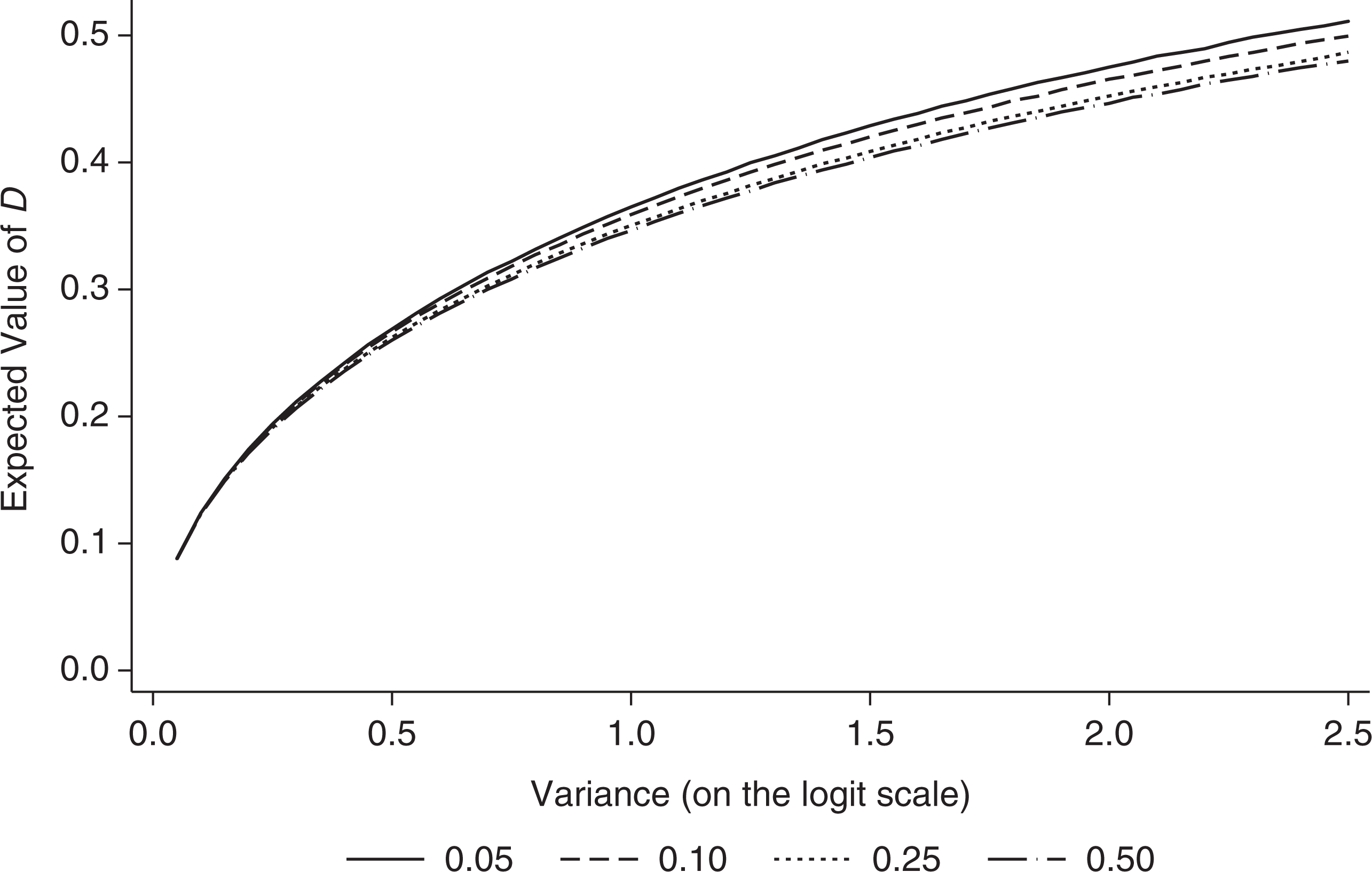
Expected value of D based on underlying proportions plotted against the variance on the logit scale for different overall proportions.

The figure shows that the expected value of D varies slightly according to the overall proportion of FSM students. Thus, even if there has been no underlying change in segregation, a large change in the overall proportion would lead to an apparent change in segregation as measured by the simulated descriptive indices. It can be argued that it is more reasonable to have a segregation measure that does not depend on the underlying proportion, in which case a common value of the underlying proportion can be imposed.

The expected value of D, holding the overall proportion constant, is a monotonically increasing function of the variance and so converting between the logit and index scale is an order preserving transformation. This means that when we specify, for example, a model with separate school-level variances for a series of cohorts, the rank ordering of the point estimates of D simulated from the estimated variances will be the same as the rank order of the estimated variances themselves. Likewise, differences shown to be significant on the logit scale will also be significant on the index scale. Thus, to establish whether segregation has significantly increased over time, or to establish in which areas segregation is highest, inferences can be made solely in terms of variance parameters. Further, the Appendix demonstrates that the expected values of all common segregation indices are monotonically increasing functions of one another.

It can also be argued that choice of index is unimportant for comparing changes in segregation. For example, to establish which of the two areas experienced a greater increase in segregation, we would compare the increase in segregation for the first area with that for the second. The approximately linear relationship between the two scales for all but large differences in segregation means that it does not matter which index is used, since the ratio of the two increases will be approximately the same. Choice of index will only be important when the increases in segregation being compared relate to very different parts of the logit/index scales. However, it does not seem substantively wise to compare areas that are so fundamentally different.

5. Social Segregation Among London Schools: An Application

In England, pro-market education reforms of the secondary schooling system (ages 11 to 16), from 1988 onward, set up new incentives and opportunities for schools and parents. Parents were given greater opportunity to choose a school for their children and were provided with school level examination results in the form of published school league tables (Leckie & Goldstein, 2009). This has created a continuing debate about whether social diversity or segregation among schools has changed as a result of parents exercising choice and continuing modifications to the curriculum and status of schools. In this debate, interest has focused on calculating segregation index scores which summarize the variation among schools in the proportion of FSM students. These scores are then compared across cohorts, to describe whether segregation, at the national and area scales has increased or decreased over time (e.g., Allen & Vignoles, 2007) and across areas, to describe where in England segregation is highest and lowest.

5.1. The Data

The data are taken from the Annual School Census (ASC), a census of all schools in the state education system in England. We narrow our attention to schools in London and focus on the cohort of students who entered secondary schooling in 2002 and the cohort who entered in 2008. These are the first and last cohorts for which we have data. Schools in London come under the responsibility of 32 LAs: 12 in inner London and 20 in outer London. Across the two cohorts, there are 416 schools and the vast majority of these are present for both cohorts. There are, on average, 185 students in each school cohort, but in some cases there are as few as 100 or as many as 300.

For each student, we have a binary response: whether they are eligible (1) or not (0) for FSM. However, for computational efficiency, we will estimate models for the equivalent binomial response: the proportion eligible for FSM in each school cohort. We will not be including student-level predictor variables in our models and so no information is lost by merging the student level data into school-cohort proportions. It is also helpful to illustrate these models in terms of proportions as many data used in segregation studies are released, for confidentially reasons, as proportions or counts (Subramanian, Duncan & Jones, 2001). The mean proportion in 2002 was 0.28 and in 2008 it was 0.27.

5.2. Estimation Details

We use MCMC estimation methods as implemented in MLwiN (Browne, 2009; Rasbash, Charlton, Browne, Healy & Cameron, 2009). We ran MLwiN through the Stata statistical software package by using the user written runmlwin Stata command (Leckie and Charlton, 2011). Estimates obtained using the quasi-likelihood methods in MLwiN were used as initial values. The models were run for a burn-in of 5,000 iterations followed by a monitoring chain of 50,000 iterations. We used hierarchical centering (Browne, 2009; Browne, Steele, Golalizadeh, & Green, 2009) to produce chains that exhibit better mixing and the standard default prior distributions provided by MLwiN. The default prior distribution used for the variance parameters is an inverse gamma $Γ^{- 1} (0.001, 0.001)$ and for covariance matrices is an inverse Wishart with parameters equal to the quasi-likelihood estimates. In the case of small samples, the choice of default priors may be important (Browne, 1998), but for our data the number of schools is sufficiently large that altering the default prior to be uniform does not appreciably change the values for the school estimates. The small number of LA units considered in our illustrative application means that altering the default prior to be uniform does lead to small increases in the LA estimates, but these changes do not alter our substantive conclusions. Informal visual assessments of the parameter chains and standard MCMC convergence diagnostics suggested that the sampler was run for sufficiently long. The MCMC approach allows the fit of models to be compared via the deviance information criterion (DIC; Spiegelhalter, Best, Carlin, & van der Linde, 2002): models with smaller DIC values are preferred to those with larger values, with differences of 10 or more considered substantial. Where we simulate index scores from the model parameters, we simulate these from the MCMC point estimates rather than the MCMC chains of parameter estimates. Although the latter approach is preferable (see Section 4.1), in this instance, the large scale nature of our data meant it would be computationally burdensome.

5.3. The Two-Level Variance Components Binomial Response Model for Proportions

We first fit the Model 1 (Equation 1), the simple two-level variance components binomial response model for proportions, to the 2008 cohort of students. This model measures the degree of segregation among London schools for our most recent year of data. Estimates are shown in Table 1 .

Table 1.

Parameter Estimates for Model 1

Parameter	Estimate (Standard error)
$β_{0}$ Intercept	−1.220 (0.054)
$σ_{u}^{2}$ School variance	1.087 (0.087)
$D_{u}$ School dissimilarity index	0.366 (0.341, 0.391)
DIC	3,018.161

Note: A 95% interval is reported for $D_{u}$ rather than a standard error.

In the median school, the proportion of students in poverty is predicted as $anti - logit (- 1.220) = 0.228$ . The degree of segregation among schools is estimated as 1.087. Comparing the DIC to a model without school random effects (not shown) confirms the existence of segregation across London schools.

If we use the simulation method described in Section 4.1 to calculate the dissimilarity index based on the parameter estimates of $β_{0}$ and $σ_{u}^{2}$ , we obtain a value of 0.366 with a 95% interval of [0.341, 0.391]. This suggests that on average, 37% of FSM students would have to move to other schools in London in order to achieve an even distribution of FSM students across all schools in the city. The dissimilarity index score based on the observed proportions is similar with a value of 0.355.

5.4. Adding LAs as an Additional Level of Analysis

Next we fit Model 2 (Equation 2), a three-level model that measures segregation simultaneously at the LA and school levels. Fitting the model gives the estimates shown in Table 2 . Model 2 offers only a very slight improvement in fit over Model 1, which did not include the LA random effects (the DIC is reduced by 2 points). The LA variance is almost as large as the school variance and their sum is similar to the estimate for the school variance in Model 1. Thus, almost half of the segregation previously seen as between schools in Model 1 is better described as segregation between LAs. One interpretation of the high degree of LA level segregation is that it reflects substantial differences in family income across LAs in London. However, not all children in London are schooled in the LA in which they live and so the degree of LA level segregation in the education system reported here might actually differ from the corresponding degree of LA level residential segregation. It is possible to extend the current model to explore whether the schooling system exacerbates or mitigates the degree of residential social segregation and we return to this and other possible extensions in the Discussion. Table 2 shows that the school level variance is also large suggesting that there is also considerable social segregation between the schools within each LA. Thus, even within LAs, where schools are located only a short distance apart, there is substantial variation in the proportion of poor students across schools. The LA variance is estimated less precisely than the school variance reflecting the low number of units at the LA level (32 LAs) compared to at the school level (380 schools).

Table 2.

Parameter Estimates for Model 2

Parameter	Estimate (Standard Error)
$β_{0}$ Intercept	−1.157 (0.134)
$σ_{v}^{2}$ LA variance	0.516 (0.157)
$σ_{u}^{2}$ School variance	0.582 (0.050)
$D_{v}$ Simulated LA dissimilarity index	0.267 (0.199, 0.340)
$D_{u}$ Simulated School dissimilarity index	0.283 (0.262, 0.304)
DIC	3,016.454

Note: A 95% interval, rather than a standard error, is reported for each simulated dissimilarity index.

As before, we use the simulation method to report the estimated variances in terms of the dissimilarity index. The results show a score of 0.267 for LA level segregation compared to 0.283 for school level segregation. Thus, just as the LA point estimate of the variance was smaller than the school variance, the simulated LA dissimilarity index score point estimate is smaller than that for schools. The scores suggest that 27% of FSM children in London would have to move to schools in other LAs in order to eradicate segregation between LAs (but not within LAs). To instead eradicate segregation within LAs (but to leave segregation between LAs unchanged), on average 28% of FSM students in each LA would have to move to other schools within their LA. The 95% interval for the LA level dissimilarity index is considerably wider than that for the school level index reflecting the lower precision for the LA variance compared to that for the school variance.

5.5. Adding a Second Cohort as an Additional Response Variable

Next we fit Model 3 (Equation 3), the two cohort version of Model 2, which measures changes in LA and school level segregation over time. We fit the model to the earliest and latest cohorts for which we have data: 2002 and 2008. Recall that these two cohorts contain entirely different children: The first cohort contains those children that entered secondary schooling in 2002; the second contains those that entered in 2008. The estimates are shown in Table 3 .

Table 3.

Parameter Estimates for Model 3

Parameter	Estimate (Standard Error)
$β_{0}^{(1)}$ 2002 Intercept	−1.171 (0.159)
$β_{0}^{(2)}$ 2008 Intercept	−1.136 (0.134)
LA level
$σ_{v (1)}^{2}$ 2002 LA variance	0.743 (0.215)
$σ_{v (12)}$ 2002 and 2008 LA covariance	0.615 (0.179)
$σ_{v (2)}^{2}$ 2008 LA variance	0.523 (0.153)
School level
$σ_{u (1)}^{2}$ 2002 school variance	0.782 (0.067)
$σ_{u (12)}$ 2002 and 2008 school covariance	0.634 (0.054)
$σ_{u (2)}^{2}$ 2008 school variance	0.626 (0.052)
$D_{v (1)}$ 2002 Simulated LA dissimilarity index	0.312 (0.232, 0.398)
$D_{v (2)}$ 2008 Simulated LA dissimilarity index	0.268 (0.200, 0.342)
$D_{u (1)}$ 2002 Simulated school dissimilarity index	0.321 (0.298, 0.344)
$D_{u (2)}$ 2008 Simulated school dissimilarity index	0.292 (0.271, 0.313)
DIC	5,899.353

Note: A 95% interval, rather than a standard error, is reported for each simulated dissimilarity index.

In 2008, the median school had a slightly higher proportion of FSM students than in 2002 (24.3% compared to 23.7%); however, the MCMC chain for the difference in these parameter estimates shows this can be explained by random variation.

The 2008 LA variance is smaller than the 2002 variance and so LA level segregation reduces between the two cohorts. The school level variance also reduced over this period indicating that segregation within LAs also fell. Comparisons of the DIC to simpler models that restrict the two LA level variances to be equal and the two school level variances to be equal (not shown) indicate that the model that does not constrain these pairs of variances to be equal is to be preferred, so both the LA and the school reductions in segregation shown in this model are statistically significant. The LA level covariance implies a very high correlation of .99 = $(0.615 / \sqrt{0.743 \times 0.523})$ between the 2002 and 2008 LA random effects. Thus, there has been almost no reordering of London LAs in terms of the proportion of FSM students they teach over the 7-year period. The school level correlation is smaller but is still extremely high (.91). Thus, even within LAs, there has been little change in the ordering of schools; there is a great continuity in terms of poverty for London schools over time.

We again use the simulation method to report the estimated variances in terms of the dissimilarity index. The results show a score of 0.312 for LA level segregation in 2002 which reduced to 0.268 in 2008. At the school level, segregation dropped from 0.321 to 0.292. The drop in the simulated index scores suggest that the proportion of FSM students that would have to move to schools in other LAs in order to eradicate LA segregation dropped from 31% to 27% between the two cohorts. The equivalent drop at the school level was less marked: On average, 32% of the 2002 FSM students would have to move to other schools within their LAs to eradicate segregation within LAs compared to 29% in 2008. To test whether this drop in school level segregation was significant, we follow the method outlined in Section 4.1 and calculate the difference between the 2008 and 2002 index scores at each iteration of the MCMC algorithm. The 95% interval for the difference in scores (−0.037, −0.021) does not include 0 and so the degree of school segregation in 2008 is judged significantly less at the 5% level than it was in 2002.⁴

5.6. Modeling Segregation as a Function of LA Predictor Variables

In Models 2 and 3, we found that within LAs, FSM students were segregated across schools. One explanation is the way students are admitted to schools. Seven of the outer London LAs operate a selective admissions system whereby initially high achieving students are sent to “grammar schools” based on their performance in entrance exams. These schools select on ability and since children’s test scores tend to be positively associated with family income, grammar schools tend to teach lower proportions of FSM students than neighboring nongrammar schools. It therefore seems likely that schools in selective LAs might be more segregated in terms of poverty than those in nonselective LAs. To explore this, we fit Model 4 (Equation 4) and use the three binary LA level indicator variables to distinguish between three groups of LAs: (a) the 12 nonselective LAs in inner London; (b) the 13 nonselective LAs in outer London; and (c) the seven selective LAs in outer London. The nonselective LAs in outer London are distinguished from those in inner London to provide a fairer comparison group for the group of selective LAs since the latter group are only located in outer London. Inner London is also considerably more deprived than outer London and so segregation measures are often reported separately for these two areas (see, e.g., Johnston, Burgess, Harris, & Wilson, 2008). The results are presented in Table 4 .

Table 4.

Parameter Estimates for Model 4

Parameter	Estimate (Standard Error)
$β_{1}^{(1)}$ 2002 Intercept for schools in inner London	−0.402 (0.169)
$β_{1}^{(2)}$ 2008 Intercept for schools in inner London	−0.508 (0.140)
$β_{2}^{(1)}$ 2002 Intercept for schools in nonselective LAs in outer London	−1.290 (0.166)
$β_{2}^{(2)}$ 2008 Intercept for schools in nonselective LAs in outer London	−1.199 (0.138)
$β_{3}^{(1)}$ 2002 Intercept for schools in selective LAs in outer London	−2.140 (0.232)
$β_{3}^{(2)}$ 2008 Intercept for schools in selective LAs in outer London	−2.007 (0.198)
LA level
$σ_{v (1)}^{2}$ 2002 LA variance	0.284 (0.095)
$σ_{v (12)}$ 2002 and 2008 LA covariance	0.222 (0.077)
$σ_{v (2)}^{2}$ 2008 LA variance	0.195 (0.066)
School level for all LAs in inner London
$σ_{u 1 (1)}^{2}$ 2002 school variance	0.571 (0.086)
$σ_{u 1 (12)}$ 2002 and 2008 school covariance	0.416 (0.065)
$σ_{u 1 (2)}^{2}$ 2008 school variance	0.415 (0.063)
School level for nonselective LAs in outer London
$σ_{u 2 (1)}^{2}$ 2002 school variance	0.662 (0.088)
$σ_{u 2 (12)}$ 2002 and 2008 school covariance	0.514 (0.069)
$σ_{u 2 (2)}^{2}$ 2008 school variance	0.504 (0.066)
School level for selective LAs in outer London
$σ_{u 3 (1)}^{2}$ 2002 school variance	1.293 (0.205)
$σ_{u 3 (12)}$ 2002 and 2008 school covariance	1.166 (0.182)
$σ_{u 3 (2)}^{2}$ 2008 school variance	1.171 (0.185)
Simulated school level dissimilarity index scores
$D_{u 1 (1)}$ 2002 School dissimilarity index (LAs in inner London)	0.278 (0.243,0.314)
$D_{u 1 (2)}$ 2008 School dissimilarity index (LAs in inner London)	0.242 (0.211,0.275)
$D_{u 2 (1)}$ 2002 School dissimilarity index (nonselective LAs in outer London)	0.300 (0.265,0.335)
$D_{u 2 (2)}$ 2008 School dissimilarity index (nonselective LAs in outer London)	0.266 (0.237,0.296)
$D_{u 3 (1)}$ 2002 School dissimilarity index (selective LAs in outer London)	0.400 (0.347,0.458)
$D_{u 3 (2)}$ 2008 School dissimilarity index (selective LAs in outer London)	0.383 (0.332,0.440)
DIC	5,898.704

Note: A 95% interval, rather than a standard error, is reported for each simulated dissimilarity index.

This model offers a slight improvement in fit over Model 3. We first consider the results for the 2008 cohort. The estimates show that 38% of students in the median school located within inner London are eligible for FSM, compared to 23% in nonselective outer London LAs and just 12% in the selective LAs. These estimates clearly show the higher degree of poverty seen in inner London schools. Adjusting for these differential rates of poverty leads to a substantial reduction in the estimates of the LA variances compared to those reported in Model 3. Thus, while there are large differences in poverty between these three types of LAs, within each type, the LAs are relatively similar. At the school level, the estimated variance parameters show that schools in inner London LAs are typically less segregated than those in outer London LAs. For schools in outer London LAs, we see that those located within selective LAs are by far the most segregated in London. Thus, it appears that allowing schools to select on ability indirectly leads them to select on poverty and therefore imbalances schools in terms of their social mix.

Comparing the 2008 results to those for 2002 shows that the percentage of FSM students taught in inner London decreased over the 6 years (the percentage in the median school dropped from 40% to 38%) while the percentage taught in outer London increased slightly (from 22% to 23% in the nonselective LAs and from 11% to 12% in the selective LAs). There is therefore some suggestion that inner and outer London have become more similar (i.e., less segregated) in terms of the proportion of FSM students taught in their schools. The LA variance also decreased over the period suggesting that, within each type, LAs have become more similar (i.e., less segregated) in terms of the proportion of FSM students they teach. Further, all three school variances also decreased over the period suggesting that FSM students became less segregated across schools within all three types of LA. In sum, these results indicate that schooling in London has become less segregated at a range of levels over the 6-year period.

Finally, we use the simulation method to present the estimated variances in terms of the dissimilarity index. To conserve space, Table 4 presents the simulated index scores at the school level only. For the 2008 (2002) cohort, the mean index scores are 0.242 (0.278) for inner London, 0.266 (0.300) for the nonselective outer London LAs, and 0.383 (0.400) for the selective outer London LAs. Thus, we again see that segregation among schools is considerably higher for those located in selective LAs than for those in nonselective LAs and that all three types of LA became less segregated over the period.

6. Discussion

The multilevel modeling approach to segregation is essentially concerned with modeling the underlying proportions of interest and treats the observed proportions as just one stochastic realization from an underlying social process. This approach therefore allows us to make statistical inferences about the underlying patterns of segregation and how these change over time: we can make inferences and construct interval estimates in the usual ways. Furthermore, patterns of segregation can be modeled simultaneously at multiple levels in the data, for example, at multiple organizational levels in an education system or at multiple spatial scales. Furthermore, we can model segregation as a function of predictor variables, such as area characteristics. In doing so, the multilevel modeling approach is not just able to measure patterns of segregation but offers a way to explain the existence of such patterns and why they change over time. These possibilities are not easily available in the descriptive index approach and it is therefore difficult to see how that approach can further extend our understanding of segregation.

However, if values of a traditionally used index are still desired, for example, for the purpose of presenting findings to a general audience, we have shown how these can be simulated from the estimated parameters of the multilevel model. It is then possible to make statistical inferences about the underlying social process in terms of the chosen index and we have illustrated how this can be done. The advantages of using a model for the analysis and, if desired, simulating index scores for the purpose of presenting findings strongly suggest that this should become the standard approach. Our own view, however, is that there may be little to be gained from simulating such indices when there are straightforward interpretations of the estimated model parameters themselves. Indeed, the simulated index scores for all common segregation indices are monotonically increasing functions of the model variance parameters and so simulating index scores from the variances are order preserving transformations—the rankings of the areas or years that are being examined are unaltered. Further, the relationship between simulated index scores and the variance on the logit scale is approximately linear for all but large differences in segregation and so when, for example, the increases in segregation experienced by two areas are compared, the increase experienced in one area relative to the other is approximately the same whether we choose to work with the estimated variances or simulated index scores; either way, we arrive at the same conclusions.

The multilevel modeling approach to segregation can be extended in many ways beyond those covered in this paper. We can fit nonhierarchical, cross-classified models (Rasbash & Goldstein, 1994; Raudenbush, 1993) to disentangle residential and school segregation when schools are not nested within neighborhoods or vice versa. We can fit models with multivariate responses to jointly model social segregation and, for example, academic segregation in relation to student achievement scores. Unlike the descriptive approach to segregation, nonbinary response types, such as achievement scores measured on a continuous or ordinal scale, pose no problems for the multilevel modeling approach. Models with unordered multinomial responses can also be fitted to model multigroup segregation, where interest lies in modeling segregation among three or more subgroups of the population (Reardon & Firebaugh, 2002). Finally, models with spatially correlated random area effects can be fitted to model spatial segregation (Reardon & O’Sullivan, 2004).

While our discussion has been in the context of social segregation among schools, the statistical issues we discuss are equally relevant to race and ethnic and other kinds of segregation as well as to measuring segregation among different types of institution or segregation among neighborhoods. Further work is currently underway, extending the multilevel approach to modeling multigroup ethnic segregation among schools and ethnic spatial segregation among neighborhoods.

Appendix

While the dissimilarity index D is the most widely used segregation index (see Section 2.2), many other indices exist. The Gini index (Duncan & Duncan, 1955) and the isolation index (Bell, 1954; Lieberson, 1981) are also commonly used segregation indices while Theil's information-based entropy index (Theil, 1972; Theil and Finizza, 1971) was recently recommended as satisfying a range of desirable index properties (Reardon & Firebaugh, 2002). The Gini index 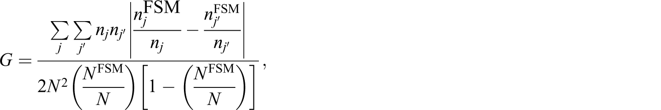$G$ is given by

G = \frac{\sum_{j} \sum_{j^{'}} n_{j} n_{j^{'}} |\frac{n_{j}^{FSM}}{n_{j}} - \frac{n_{j^{'}}^{FSM}}{n_{j^{'}}}|}{2 N^{2} (\frac{N^{FSM}}{N}) [1 - (\frac{N^{FSM}}{N})]},

where

n_{j}^{FSM}

and

n_{j^{'}}^{FSM}

are the number of FSM students in schools

j

and

j^{'}

, respectively, while

n_{j}

and

n_{j^{'}}

are the total number of students in the two schools.

N^{FSM}

is the total number of FSM students across all schools and

N

is the total number of students of either type across all schools. The index is bounded by 0 (no segregation, all schools have the same observed proportion of FSM students) and 1 (complete segregation, no schools are observed with both FSM and non-FSM children).

The isolation index $I$ is given by

I = \sum_{j} [(\frac{n_{j}^{FSM}}{N^{FSM}}) (\frac{n_{j}^{FSM}}{n_{j}})] .

The index is bounded from below by

N^{FSM} / N

, the overall proportion of FSM students (no segregation), and 1 (complete segregation). The value of I provides a useful interpretation, as the probability that a random FSM student attends a school with another FSM student. The index is also interpreted as the mean exposure of FSM students to other FSM students.

Theil’s information-based entropy index $H$ is given by

H = \sum_{j}^{} \frac{n_{j} (E - E_{j})}{N E},

where

E

defines the diversity across all schools and is termed the entropy.

E = \frac{N^{NONFSM}}{N} ln (\frac{N}{N^{NONFSM}}) + \frac{N^{FSM}}{N} ln (\frac{N}{N^{FSM}}),

and

E_{j}

defines the diversity within school

j

E_{j} = \frac{n_{j}^{NONFSM}}{n_{j}} ln (\frac{n_{j}}{n_{j}^{NONFSM}}) + \frac{n_{j}^{NONFSM}}{n_{j}} ln (\frac{n_{j}}{n_{j}^{FSM}}) .

Like D and G, H is bounded by 0 (no segregation, all schools have the same observed proportion of FSM students) and 1 (complete segregation, no schools are observed with both FSM and non-FSM children).

Figure 3 corresponds to Figure 1 (see Section 2.2) and shows the expected value of D, G, I, and H, based on observed proportions, when there is no underlying segregation. The expected values are plotted against school size when the overall FSM proportion is 0.25. The figure shows that all four indices are biased upward as the observed proportions include the effects of sampling variability. We note that Theil’s information-based entropy index suffers from the smallest bias and this is expected, given that the index has been shown to satisfy a range of desirable index properties (Reardon and Firebaugh, 2002).

Figure 3.

Expected values of D, G, I, and H based on observed proportions plotted against school size when there is no underlying segregation.

Figure 4 corresponds to Figure 2 (see Section 4.2) and shows the expected value of D, G, I, and H, based on underlying proportions for different degrees of underlying segregation. The expected values are plotted against the variance on the logit scale for when school sizes are 200 students per school and for when the overall FSM proportion is 0.25. The figure shows that the expected value of each index, holding the overall proportion constant, is a monotonically increasing function of the variance. Thus converting between any pair of simulated indices is an order preserving transformation and, as discussed in Section 4.2, makes the choice of index after fitting the multilevel model arbitrary.

Figure 4.

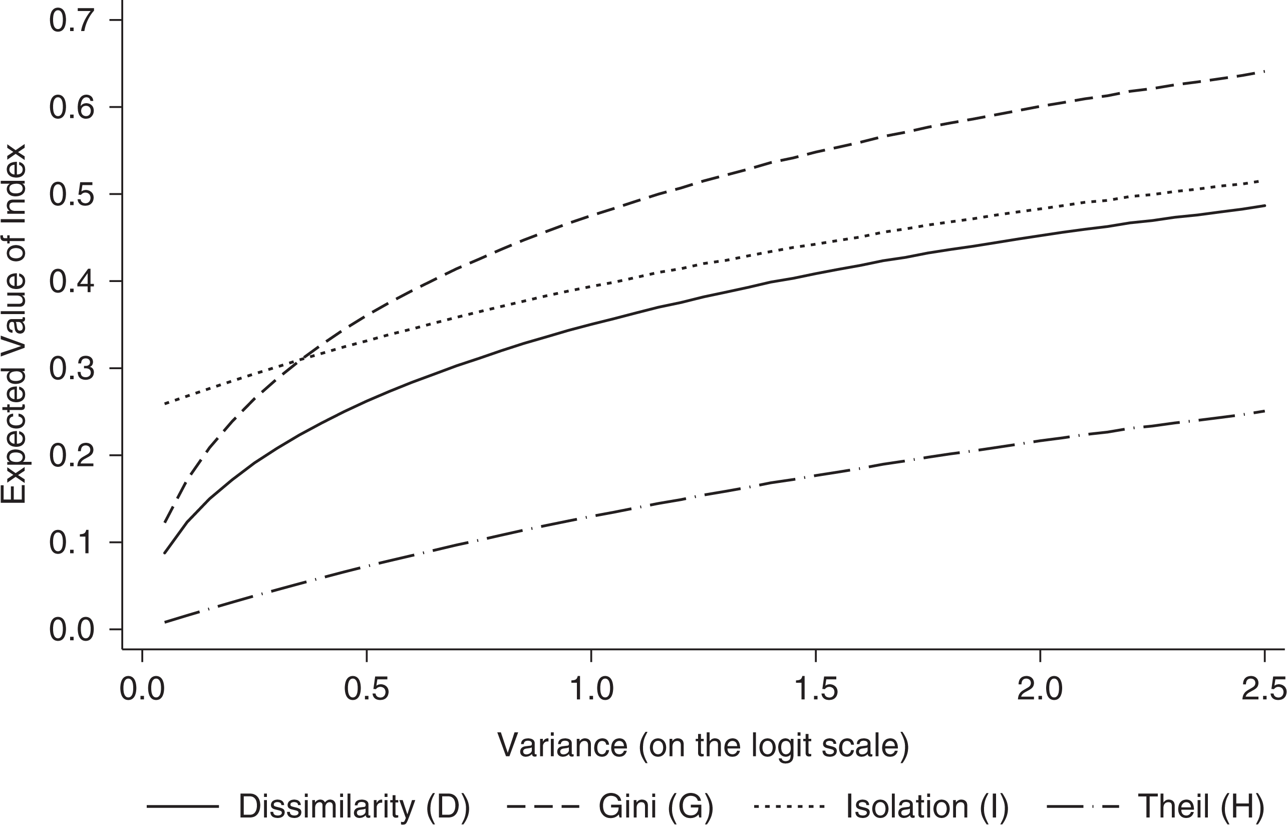
Expected value of D, G, I, and H based on underlying proportions plotted against the variance on the logit scale.

Footnotes

Acknowledgments

The authors are grateful for the very helpful and detailed comments that were provided by the three referees and the Editor. This work was funded under the UK Economic and Social Research Council’s National Centre for Research Methods program.

Notes

References

Allen

Vignoles

(2007). What should an index of school segregation measure?. Oxford Review of Education, 33, 643–668.

Bell

(1954). A probability model for the measurement of ecological segregation. Social Forces, 32, 357–364.

Browne

W. J.

(1998). Applying MCMC methods to multilevel models. PhD Thesis, Department of Mathematical Sciences, University of Bath, Bath.

Browne

W. J.

(2009). MCMC estimation in MLwiN, v2.10 Bristol, UK: Centre for Multilevel Modelling, University of Bristol.

Browne

W. J.

Steele

Golalizadeh

Green

M. J.

(2009). The use of simple reparameterizations to improve the efficiency of Markov chain Monte Carlo estimation for multilevel models with applications to discrete time survival models. Journal of the Royal Statistical Society: Series A, 172, 579–598.

Carrington

W. J.

Troske

K. R.

(1997). On measuring segregation in samples with small units. Journal of Business & Economic Statistics, 15, 402–409.

Clotfelter

C. T.

(1999). Public school segregation in metropolitan areas. Land Economics, 75, 487–504.

Cortese

C. F.

Falk

R. F.

Cohen

J. K.

(1976). Further considerations on the methodological analysis of segregation indices. American Sociological Review, 41, 630–637.

Duncan

O. D.

Duncan

(1955). A methodological analysis of segregation indices. American Sociological Review, 20, 210–217.

10.

Goldstein

. (2010). Multilevel statistical models (4th ed.). Wiley.

11.

Goldstein

Noden

(2003). Modelling social segregation. Oxford Review of Education, 29, 225–237.

12.

Hutchens

(2004). One measure of segregation. International Economic Review, 45, 555–578.

13.

Jahn

Schmid

C. F.

Schrag

(1947). The measurement of ecological segregation. American Sociological Review, 12, 293–303.

14.

James

D. R.

Taeuber

K. E.

(1985). Measures of segregation. Sociological Methodology, 15, 1–32.

15.

Johnston

Burgess

Harris

Wilson

(2008). “Sleep-walking towards segregation?” The changing ethnic composition of English schools, 1997–2003: An entry cohort analysis. Transactions of the Institute of British Geographers, 33, 73–90.

16.

Leckie

Charlton

(2011). runmlwin: Stata module for fitting multilevel models in the MLwiN software package. Centre for Multilevel Modelling, University of Bristol.

17.

Leckie

Goldstein

(2009). The limitations of using school league tables to inform school choice. Journal of the Royal Statistical Society Series A; Statistics in Society, 172, 835–851.

18.

Lieberson

(1981). An asymmetrical approach to segregation. In Peach

Robinson

Smith

(Eds.), Ethnic segregation in cities Athens: The University of Georgia Press.

19.

Massey

D. S.

Denton

N. A.

(1988). The dimensions of residential segregation. Social Forces, 67, 281–315.

20.

Massey

D. S.

Denton

N. A.

(1993). American apartheid: segregation and the making of the underclass Cambridge, MA: Harvard University Press.

21.

Massey

D. S.

Hajnal

Z. L.

(1995). The changing geographic structure of Black-White segregation in the United-States. Social Science Quarterly, 76, 527–542.

22.

Massey

D. S.

Rothwell

Domina

(2009). The changing bases of segregation in the United States. Annals of the American Academy of Political and Social Science, 626, 74–90.

23.

Ransom

M. R.

(2000). Sampling distributions of segregation indexes. Sociological Methods & Research, 28, 454–475.

24.

Rasbash

Goldstein

(1994). Efficient analysis of mixed hierarchical and cross-classified random structures using a multilevel model. Journal of Educational and Behavioral Statistics, 19, 337–350.

25.

Rasbash

Charlton

Browne

W. J.

Healy

Cameron

(2009). MLwiN Version 2.1. Centre for Multilevel Modelling, University of Bristol.

26.

Raudenbush

S. W.

(1993). A crossed random effects model for unbalanced data with applications in cross-sectional and longitudinal research. Journal of Educational and Behavioral Statistics, 18, 321–349.

27.

Raudenbush

S. W.

Bryk

A. S.

(2002). Hierarchical linear models: Applications and data analysis methods 2nd ed. Newbury Park, CA: Sage.

28.

Reardon

S. F.

Firebaugh

(2002). Measures of multigroup segregation. Sociological Methodology, 32, 33–67.

29.

Reardon

S. F.

O’Sullivan

(2004). Measures of spatial segregation. Sociological Methodology, 34, 121–162.

30.

Spiegelhalter

D. J.

Best

N. G.

Carlin

B. P.

van der Linde

(2002). Bayesian measures of model complexity and fit. Journal of the Royal Statistical Society: Series B, 64, 583–639.

31.

Subramanian

S. V.

Duncan

Jones

(2001). Multilevel perspectives on modeling census data. Environment and Planning A, 33, 399–417.

32.

Taeuber

K. E.

Taeuber

A. F.

(1965). Negroes in cities: Residential segregation and neighbourhood change Chicago, IL: Aldine.

33.

Theil

(1972). Statistical decomposition analysis Amsterdam, Netherlands: North-Holland.

34.

Theil

Finizza

A. J.

(1971). Note on measurement of racial integration of schools by means of informational concepts. Journal of Mathematical Sociology, 1, 187–193.

35.

Tranmer

Steel

D. G.

(2001). Ignoring a level in a multilevel model: Evidence from UK census data. Environment and Planning A, 33, 941–948.

36.

White

M. J.

(1986). Segregation and diversity measures in population-distribution. Population Index, 52, 198–221.

37.

Wright

J. K.

(1937). Some measures of distributions. Annals of the Association of American Geographers, 27, 177–211.

38.

Zoloth

B. S.

(1976). Alternative measures of school segregation. Land Economics, 52, 278–298.