Estimating a Meaningful Point of Change

Abstract

Longitudinal studies are increasingly common in psychological research. Characterized by repeated measurements, longitudinal designs aim to observe phenomena that change over time. One important question involves identification of the exact point in time when the observed phenomena begin to meaningfully change above and beyond baseline fluctuations. The authors introduce a nonparametric modeling framework to estimate the change-point of interest using derivatives of the underlying regression function for an outcome variable across time. The estimator of Huh and Carriere (HC) consistently performed acceptably when using a plug-in bandwidth in a Monte Carlo simulation study. It was shown that the estimator performed well with a minimum number of 15 design points. This procedure was applied to longitudinal data collected on performance anxiety. Results suggest that the HC estimator combined with plug-in bandwidth selection provides an efficient strategy for investigating a possible change-point at which an observed outcome variable starts changing across time.

Keywords

change-point estimation bandwidth selection nonparametric regression long-range dependent errors short-range dependent errors

Longitudinal studies are increasingly common in psychological research. Characterized by repeated measurements, longitudinal designs aim to observe outcome variables that change over time, regardless of whether the obtained data are molar or molecular in nature. Within the dynamic nature of these data, one important question involves identification of the time point when the observed outcome variable begins to meaningfully change above and beyond baseline fluctuations.

Consider the two following hypothetical situations, each of which explicitly or implicitly seeks to identify the point of meaningful change. (a) In a typical ecological momentary assessment (EMA) design (Gloster et al., 2008; Kashdan & Steger, 2006; Shiffman, Stone, & Hufford, 2008; Stone, Schwartz, Broderick, & Shiffman, 2005; Stone & Shiffman, 2002), multiple variables are assessed multiple times per day in one’s natural environment. Analyses of EMA data are commonly focused on detecting predictor variables for a meaningful fluctuation in the outcome variable across time. In this constellation, the time point at which fluctuations in the outcome variable rises above baseline variation may provide important information regarding the focal phenomena. (b) A typical psychophysiological experiment may examine the interaction between physiological variables and standardized events across a battery of paradigms. For example, heart rate, blood pressure, and electrodermal activation (EEG) are collected during a standardized experiment in patients with an anxiety disorder. The aim of the experiment is to investigate the course of physiological characteristics of patients in a standardized setting. If a meaningful change in any variable appears, it may be of crucial importance to identify the time point when the change in a parameter started in order to find out what precipitated the observed changes in the outcome variable.

The particular time point at which an observed outcome variable begins to change is denoted by θ. The slope of the hypothesized regression curve starts changing at the change-point θ. There are several reasons for the importance of estimating a particular change-point. In addition to proving important information about the research question, identification of the estimated change-point provides valued statistical information that can be used in the model-building process of data analyses. Information about θ influences subsequent analysis and generates new hypotheses. Predictor variables for the change itself and the magnitude of change can be identified in relation to the point of initial change. Furthermore, the change-point can also have causal implications as displayed by the two introductory examples.

The modeling framework of interrupted time-series analyses has been developed for modeling a time series with a change-point. But the change-point is assumed to be known before analyses in interrupted time-series analysis and therefore it is not a parameter to be estimated (Hartmann et al., 1980; Morgan, Griffiths, & Majeed, 2007; Wagner, Soumerai, Zhang, & Ross-Degnan, 2002).

An option to identify the change-point θ is the parametric segmented regression (SR) analysis (Muggeo, 2003). In this approach, the regression line is piecewise linear with partitions defined by the assumed change-points. This approach is flexible. It can be generalized to the generalized linear model framework with linear predictors and a finite number of change-points (Muggeo, 2003). The unknown change-point θ is also a parameter to be estimated in the SR analyses besides the simultaneously fitted regression lines. The performance of this approach depends on several assumptions that are not always met with real data. For example, a functional association between the response variable and design variable (e.g., linear) must be assumed without a priori knowledge of whether or not the stipulated relation can be met. The estimation procedure of the SR model strongly depends on the existence of the change-point θ (Muggeo, 2003). The nonconvergence of the estimation algorithm is not equivalent to the nonexistence of a possible change-point (Muggeo, 2003). A false configuration of the SR model to the data could also result in a failing of the algorithm (Muggeo, 2003). Another reason for a possible failure of the algorithm could be based on the inappropriate choice of starting values for the parameter, what is required for a nonlinear optimization algorithm (Muggeo, 2003). Therefore, different starting values for the parameter estimates could yield different estimates.

Accurate and unbiased estimation of the change-point θ is indeed a challenge and problems often arise when applying extant methods to real data. Procedures such as those described above make assumptions that often cannot be met in real data or overly rely on a trial and error strategy.

To help overcome these problems, we consider a nonparametric modeling framework for estimating the change-point θ of interest. The basic principle of estimating θ is based on nonparametric regression analysis as described in the first part of the article. Three exploratory estimation strategies are compared in a Monte Carlo simulation study. The consistently best performing estimator was then applied to longitudinal data about anticipatory performance anxiety of five musicians in the days leading up to a performance. The parametric SR analyses failed in the data about performance anxiety. It suggests that when the particular change-point θ at which an observed outcome variable starts changing across time is of interest, the nonparametric estimation procedure can be the method of choice.

Statistical Model for Estimating the Change-Point θ

The association of an outcome variable Y with a covariate T can be described by the nonparametric regression model $Y = m (T) + ϵ$ with $m (t) = E [Y | T = t]$ for $t \in {t_{1}, \dots, t_{T}}$ , where $m (\cdot)$ denotes the unknown regression function and ϵ a random variable representing the error in the equation with zero mean (Haerdle, 1990, p. 3). We assume that the first derivative of m has a jump discontinuity and is otherwise a smooth curve. Figure 1A shows a hypothetical example with noisy data $((Y_{1}, t_{1}), \dots, (Y_{T}, t_{T}))$ and its model generating regression curve m (light gray line). Typically, the covariate T represents time in longitudinal analyses as in our considerations, but other covariates are applicable. The nonparametric regression model $Y = m (T) + ϵ$ is considered asymptotically equivalent to a white noise time-series model (Brown & Low, 1996). It implies that asymptotical results from nonparametric regression analyses yield a corresponding solution in a white noise time-series model (Brown & Low, 1996).

Figure 1.

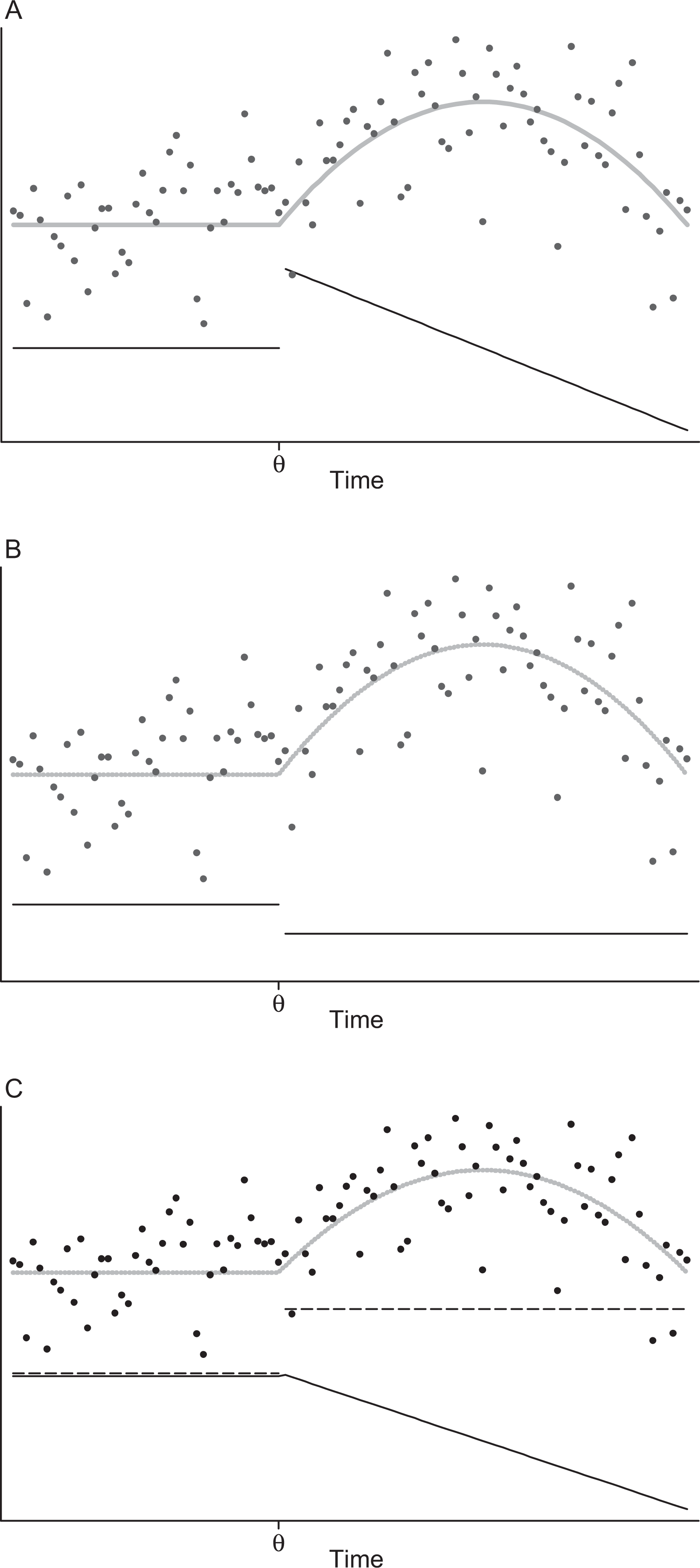
Trajectory for a hypothetical example (A: solid light gray line: Model generating regression curve m, solid black line: first derivative of m; B: solid light gray line: Model generating regression curve m, solid black line: second derivative of m; C: solid light gray line: Model generating regression curve m, solid black line: continuous part of m, dashed black line: Discontinuous part of m described by a step function).

The data are collected from the same subject over time, where the assumption of independent and identical distributed errors does not hold. The response at time t_j depends on the responses at times $t_{j - 1}, t_{j - 2}, \dots$ . We consider long-range and short-range dependent errors in our statistical model. Short-range dependent errors are characterized by the dependence of $Y_{l}$ on $Y_{k}$ for the time point k in the recent past of time point 1, in contrast to long-range dependent errors.

Nonparametric Regression Analysis

In this article, the estimator for the meaningful change-point θ is based on nonparametric regression. Nonparametric regression analysis attempts to identify a functional relationship between an outcome variable Y and a predictor variable T without needing to assume a particular functional relationship.

The local polynomial regression approach is a widely used smoothing technique besides other smoothing procedures. The regression function m is locally approximated for all t by a polynomial in the neighborhood $[t - h, t + h]$ of t, $t \in {t_{1}, \dots, t_{T}}$ and h > 0 (Haerdle, 1990, p. 39). The local polynomial approximation $({\hat{α}}_{0} (t), {\hat{α}}_{1} (t), \dots, {\hat{α}}_{υ} (t))$ , $υ \in {1, 2, \dots, q}$ of m for a date t, $t \in {t_{1}, \dots, t_{T}}$ is estimated by minimizing the least square equation

\sum_{i = 1}^{T} K (\frac{t_{i} - t}{h}) {(Y_{i} - \sum_{j = 0}^{q} {\hat{α}}_{l} (t_{i} - t)^{j})}^{2},

where q denotes the degree of the polynomial, h the smoothing parameter, and K a symmetric kernel function with support on

[- z, z], z \in ℜ

and

\int_{- z}^{z} K (u) d u = 1

. The crucial choice of the smoothing parameter h and the kernel function K will be discussed separately because of their importance in the smoothing process. The local estimate of the regression function m in date t is given by

\hat{m} (t) = {\hat{α}}_{0} (t)

and the estimate of the ν-the derivative is defined by

{\hat{m}}^{(ν)} (t) = ν! {\hat{α}}_{ν} (t)

t \in {t_{1}, \dots, t_{T}}

(Haerdle, 1990, p. 39).

Yang (2001) and Hidalgo (1997) showed that the regression function m can be estimated as in the case of independent and identically distributed errors for assumed correlated errors. It justifies the application of the local polynomial regression estimator for m in our introduced model.

Estimation of the Meaningful Change-Point θ

A more detailed study of the curve in Figure 1A shows another remarkable characteristic of m at the hypothesized change-point θ. The first derivative (solid black line) of the regression function m has a jump discontinuity at θ. This fact forms the base of the approach to estimate the change-point in longitudinal data. There are three possible strategies for estimating the location of the jump discontinuity in the first derivative of m based on properties of the curve: (a) The left-hand (lhl) and right-hand limits (rhl) of the first derivative are unequal at the point of discontinuity as highlighted by the solid black line in Figure 1A. (b) The first derivative of the regression function does not exist at θ, and its value of the second derivative is defined to be infinity as exemplified by the solid black line in Figure 1B. (c) Another option provides the separation of the “continuous part” from the “jump part” in the first derivative of the regression function m and considering the part containing the information about the jump. The idea of this approach is based on the fact that the discontinuous first derivative can be described as the sum of a continuous function (solid black line in Figure 1C) and a step function with a jump in θ (dashed black line in Figure 1C).

Estimation strategy (1)

The first derivative $m^{(1)}$ has a discontinuity at the change-point θ in the hypothesized model. The respective rhl $m_{+}^{(1)}$ and lhl $m_{-}^{(1)}$ are unequal at θ by definition of continuity of a function. The estimates for $m_{+}^{(1)}$ and $m_{-}^{(1)}$ are defined as ${\hat{m}}_{+}^{(1)} (t) = {\hat{α}}_{1} (t)$ and ${\hat{m}}_{-}^{(1)} (t) = {\hat{β}}_{1} (t)$ for $t \in<$ . The coefficient vectors $({\hat{α}}_{1} (t_{1}), \dots, {\hat{α}}_{1} (t_{T}))$ and $({\hat{β}}_{1} (t_{1}), \dots, {\hat{β}}_{1} (t_{T}))$ are determined by minimizing the least square function (1) for $\bar{t} := t_{i} - t$ and $\bar{t} := t - t_{i}$ , $t \in {t_{1}, \dots, t_{T}}$ , applying a one-sided kernel function K with support on $[0, 1]$ satisfying K(0) > 0 and K(u) ≥ 0 for $u \in (0, 1]$ . The change-point θ is estimated by choosing the date with maximum difference between the rhl and lhl, ${\hat{θ}}_{1} = arg max {t = t_{1}, \dots, t_{T} : {\hat{m}}_{+}^{(1)} (t) - {\hat{m}}_{-}^{(1)} (t)}$ . If the assumption of a jump discontinuity in the first derivative in the considered regression model is not valid, the function ${\hat{m}}_{+}^{(1)} (t) - {\hat{m}}_{-}^{(1)} (t)$ is zero for all $t \in {t_{1}, \dots, t_{T}}$ and the respective maxima of ${\hat{m}}_{+}^{(1)} - {\hat{m}}_{-}^{(1)}$ is constant zero.

The principle of comparing the rhl and lhl of the first derivative of m was introduced by Huh and Carriere (2002), Mueller (1992), and Mueller and Song (1997). The estimator ${\hat{θ}}_{1}$ is based on the presentation of Huh and Carriere (2002). Huh and Carriere observed better performance of ${\hat{θ}}_{1}$ in a Monte Carlo simulation study compared to the estimator of Mueller and Song (1997) and Mueller (1992), who applied a kernel estimator instead of local polynomial approximation.

Estimation strategy (2)

The second derivative of m does not exist and takes the value of infinity in case of a discontinuity of the first derivative in date θ. The second strategy of detecting a meaningful change is looking for dates with large values in the second derivative of m. An estimate of the second derivative is given by ${\hat{m}}^{(2)} (t) = 2 {\hat{α}}_{2} (t)$ for all $t \in {t_{1}, \dots, t_{T}}$ with ${\hat{α}}_{2} (t)$ minimizing the least square function (1). This strategy results in the estimator ${\hat{θ}}_{2} = arg max {t = t_{1}, \dots, t_{T} : {\hat{m}}^{(2)} (t)}$ for θ. When considering a regression model without a discontinuity of the first derivative $m^{(1)}$ , the second derivative does not take extreme values for any $t \in {t_{1}, \dots, t_{T}}$ .

Gijbels and Goderniaux (2004b) discussed a two-step procedure for the refinement of ${\hat{θ}}_{2}$ . Briefly, a least square estimation procedure is implemented in a small neighborhood of ${\hat{θ}}_{2}$ resulting in an improved estimator ${\hat{θ}}_{2}^{*}$ . The mathematical details and an algorithm are given in Gijbels and Goderniaux (2004b).

Estimation strategy (3)

The first derivative is modeled by a smooth function interrupted by a jump on position θ. The strategy for estimating the change-point θ is to separate the smooth curve and the jump factor as introduced by Qiu and Yandell (1998). A polynomial of second degree is fitted by the ordinary least square method in a neighborhood $[t_{j} - h, t_{j} + h]$ of $t_{j}$ for all $j = 1, \dots, T$ to obtain the coefficient vector $({\hat{β}}_{2} (t_{1}), \dots, {\hat{β}}_{2} (t_{T}))$ . The difference operator $Δ (t_{j}) = max {{\hat{β}}_{2} (t_{j}) {\hat{β}}_{2} (t_{j - ⌊n^{*} h⌋}), {\hat{β}}_{2} (t_{j}) {\hat{β}}_{2} (t_{j + ⌊n^{*} h⌋})}$ is calculated and the estimator ${\hat{θ}}_{3}$ is given by ${\hat{θ}}_{3} = arg max {t = t_{1}, \dots, t_{T} : Δ (t_{j})}$ . If a change in slope of the regression function m does not exist (first derivative of m is smooth) at θ, the maximum of $Δ (t_{j})$ is close to zero for all $t_{j} \in {t_{1}, \dots, t_{T}}$ .

The three estimation strategies provide an exploratory technique for estimating the change-point θ. Confidence intervals for the estimate $\hat{θ}$ and estimates for the number of possible change-points are also important features for real data application. This article is focused on comparing the three nonparametric estimation strategies for θ regarding its application in real data analysis. We briefly describe possible approaches for addressing the two issues in this paragraph. Confidence intervals can be calculated by applying the bootstrap principle (Carpenter & Bithell, 2000; Efron & Tibshirani, 1993) to the change-point estimators. The asymptotic distributions of the estimators for θ are unknown to date for calculating exact confidence intervals. Gijbels and Goderniaux (2004b) generalized the cross-validation criterion proposed by Mueller and Stadtmueller (1999) for estimating the number of discontinuities in derivatives. The cross-validation principle is applied to the derivative estimate with a prespecified number of discontinuities. This procedure is repeated for a set of possible discontinuities and the minima of the corresponding cross-validation quantity is the estimate of interest. Qiu and Yandell (1998) suggested another strategy. They calculated a threshold for the diagnostic function $Δ (t_{j})$ . The number of discontinuities is then given by the not neighboring design points where the function $Δ (t_{j})$ exceeds this threshold.

Choosing a Kernel Function

Besides the bandwidth parameter h, the accuracy of the estimated regression function $\hat{m}$ depends on the kernel function K. The choice of the kernel does not have critical influence to the precision of $\hat{m}$ (Hall, Lahiri, & Polzehl, 1995). Gasser, Mueller, and Mammitzsch (1985) presented optimal kernels with respect to minimizing the mean squared error of $\hat{m}$ . The estimator $\hat{m}$ is calculated by applying the kernels proposed by Gasser et al. (1985). For example, the optimal kernel function K is the Epanechnikov kernel $K (u) = \frac{3}{4} (1 - u^{2})$ for $| u | \in [0, 1]$ when estimating the regression function m by a second-degree polynomial (Gasser et al., 1985).

Bandwidth Selection

The decision about the bandwidth and therefore about the smoothness of the estimated regression curve $\hat{m}$ and its derivative ${\hat{m}}^{(1)}$ is of great importance in nonparametric regression analyses (Haerdle, 1990, p. 179). The challenging problem in the selection of an appropriate bandwidth h is balancing the two competing issues: the residuals ${\hat{ϵ}}_{i} = Y_{i} - \hat{m} (t_{i})$ , $t_{j} \in {t_{0}, \dots, t_{T}}$ of the regression model get smaller for a decreasing bandwidth h, whereas the variance of $\hat{m}$ gets larger (Haerdle, 1990, p. 179).

Several methods have been discussed for determining the smoothing parameter h in regression models with uncorrelated and correlated errors in recent years. The basic principle of all algorithms is minimizing the averaged squared error (ASE) for the considered regression curve and their derivatives, respectively. Several techniques were developed for estimating the ASE in regression models: the generalized cross-validation (GCV) method (Golub, Heath, & Wahba, 1979), plug-in methods (Chu & Marron, 1991; Opsomer, Wang, & Yang, 2001; Ruppert, 1997; Ruppert, Sheather, & Wand, 1995), and bootstrap-based methods (Faraway & Jhun, 1990; Gijbels & Goderniaux, 2004a; Taylor, 1989). The basic principles of bandwidth selection for estimating derivatives of a regression function are similar to that of estimating the regression function m itself (Haerdle, 1990, p. 194).

The cross-validation approach evaluates the ability to get an estimate for ${\hat{m}}^{(1)} (t_{i})$ by omitting the data point $(t_{i}, Y_{i})$ and $(t_{i - 1}, Y_{i - 1})$ . The estimate of the first derivative is compared to the difference quotient at $t_{j}$ instead of the observed outcome variable $Y_{j}$ for $j = 1, \dots, T$ (Haerdle, 1990, p. 194). The estimator for h is easy to implement and does not require the estimation of the error variance. Hall, Lahiri, and Polzehl (1995) introduced the leave-out cross-validation method to account for long-range or short-range dependent errors. The procedure differs in terms of leaving out a set of data points for calculating the cross-validation function. The estimate of ${\hat{m}}_{- i}^{(1)} (t_{i})$ is calculated for data $((t_{1}, Y_{1}), \dots, (t_{i - l}, Y_{i - l}), (t_{i + l}, Y_{i + l}), \dots, (t_{T}, Y_{T}))$ , what stands for omitting $(2 l - 1)$ data points.

The plug-in method for bandwidth selection aims to estimate the unknown quantities appearing in theoretical considerations of the asymptotical optimal bandwidth (Ruppert, 1997; Ruppert et al., 1995). The description of a plug-in bandwidth selector requires an exhaustive mathematical presentation; therefore, we refer to literature (Ruppert, 1997; Ruppert et al., 1995) for further reading. The plug-in-based bandwidths are less variable and asymptotical superior compared with cross validation (Loader, 1999; Ruppert et al., 1995). Ruppert (1997) proposed a well performing empirical bias bandwidth estimator for derivative estimation.

The application of the bootstrap principle establishes another possibility for estimating a bandwidth parameter by minimizing the ASE. Gijbels and Goderniaux (2004b) discussed the bootstrap principle in selecting the bandwidth h in derivative estimation. The algorithm is based on bootstrapping the centered residuals ${\hat{ϵ}}_{i} = Y_{i} - {\hat{m}}_{1} (t_{i}) - \bar{ϵ}$ ( $\bar{ϵ}$ denotes the mean value for the estimated residuals) estimated by a pilot estimator ${\hat{m}}_{1}$ . Details about the procedure are provided by Gijbels and Goderniaux (2004b). Hall et al. (1995) introduced a block bootstrap approach to account for the dependence of errors. The principle of the block bootstrap is similar compared to the bootstrap algorithm above except for the resampling step. Here, the vector of centered residuals $({\hat{ϵ}}_{1}, \dots, {\hat{ϵ}}_{T})$ is grouped into k blocks of Length 1, where k is a multiple of 1. Resampling randomly with replacement k times the k blocks results in a bootstrap version $(ϵ_{1}^{*}, \dots, ϵ_{T}^{*})$ of the residuals. The detailed theory for choosing h by block bootstrap is described in Hall et al. (1995).

Monte Carlo Simulation Study

A Monte Carlo simulation study was conducted to compare the performance of the three estimators introduced above. The study is designed to address the following issues:

What estimator best detects the meaningful change-point θ in the case of short-range and long-range dependent errors? The convergence of the three estimators of Huh and Carierre (2002), Gijbels and Goderniaux (2004b), Qiu and Yandell 1998) was shown in the case of independent and identically distributed errors. The finite sample behavior is investigated in case of correlated errors in the simulation study.

What bandwidth selection approach is best suited to obtain an accurate estimate of the change-point θ? The important issue of estimating θ has not yet been addressed in detail in the literature. Previous studies and discussions of the bandwidth parameter are not transferable to our data situation. The authors assumed a simple model with independent and identically distributed errors (Gijbels & Goderniaux, 2004b). The compared bandwidth selection criteria are the GCV, the plug-in estimator proposed by Ruppert (1997), and the block bootstrap (Hall et al., 1995) based on theoretical considerations in literature. The performance of block bootstrapping depends on the block length 1. It is a function of the range of dependency, as higher the range of dependency as larger should be the block length (Hall et al., 1995). The block length 1 varies for values of 1, 2, 5, and 10 in the simulation study.

The number of design points T is an important parameter in respect to practical application of the nonparametric change-point model. The number of longitudinally measured data is assumed to be 15, 20, 50, 100, and 500, respectively. The long-range and short-range dependent errors are given by the flexible autocovariance function used in Hall et al. (1995). The autocovariance is given by $E [ϵ_{i} ϵ_{j}] = σ^{2}^{*} e^{- λ |t_{i} - t_{j}|}$ . The parameter $σ^{2}$ is the variance of the standard normal distributed errors $ϵ_{i}$ . We study variances of .1 and .5. The range of dependency is given by the parameter λ in the autocovariance function. We model the two extreme cases of λ = 10 (long-range dependent data) and λ = 1,000 (short-range dependent data) as well as values for λ of 50.

We consider the regression functions (1) m ₁(t) = .5 for t < .5 and m ₁(t) = exp(t − .5) − 0.5 for t ≥ .5; (2) m ₂(t) = .25 for t < .5 and m ₂(t) = .7t ² + .4t − .1 for t ≥ .5; (3) m ₃(t) = .84 for t <.5 and m ₃(t) = sin (.7πt − .1) for t ≥ .5; and (4) m ₄(t) =.1t + .79 for t < .5 and m ₄(t) = sin (.7πt − .1) for t ≥ .5. The functions m ₁ and m ₂ are constant for values of t smaller than .5 and increasing values for t ≥.5. The two functions mainly differ in the magnitude of the jump in the first derivative. The regression lines m ₃ and m ₄ have a jump in the first derivative and maxima in the function itself, which provides a challenging estimation problem. Regression line m ₃ is constant and m ₄ slightly increasing for t < .5. The nonparametric estimators HC, GG, and QY are compared to the parametric SR method (Muggeo, 2003).

The results are reported in Figure 2 for the regression functions m ₂ and m ₃, a variance of .1, λ = 10 and the bandwidth selections for various values of T. Results were comparable to m ₂ and m ₃ as reported in Figure 1 for the regression functions m ₁, m ₄, and other parameter settings. The detailed results are available on request from the authors. The estimation methods HC consistently yielded acceptable bias in all simulations applying the plug-in estimator with polynomial of degree 3. The bootstrap method with block length 10 (not reported in Figure 1) resulted in acceptable estimates for values of T above 50 by comparing the rhl and lhl of the first derivative. The biases of HC were smaller than 2 measurement points in all simulation scenarios. HC underestimated the change-point θ in all cases (not shown in the figure, the absolute values of bias are reported). The bias was somewhat smaller for the bootstrap bandwidth selection with block length 10 (T ≥ 50) compared to plug-in bandwidth selection with polynomial of degree 3 (PI_2), whereas the variation (root mean square error [RMSE]) for bootstrap bandwidth selection with block length of 10 (BB_10) was larger. All bandwidth selection methods were asymptotical equivalent for large sets of measurement points (T = 500).

Figure 2.

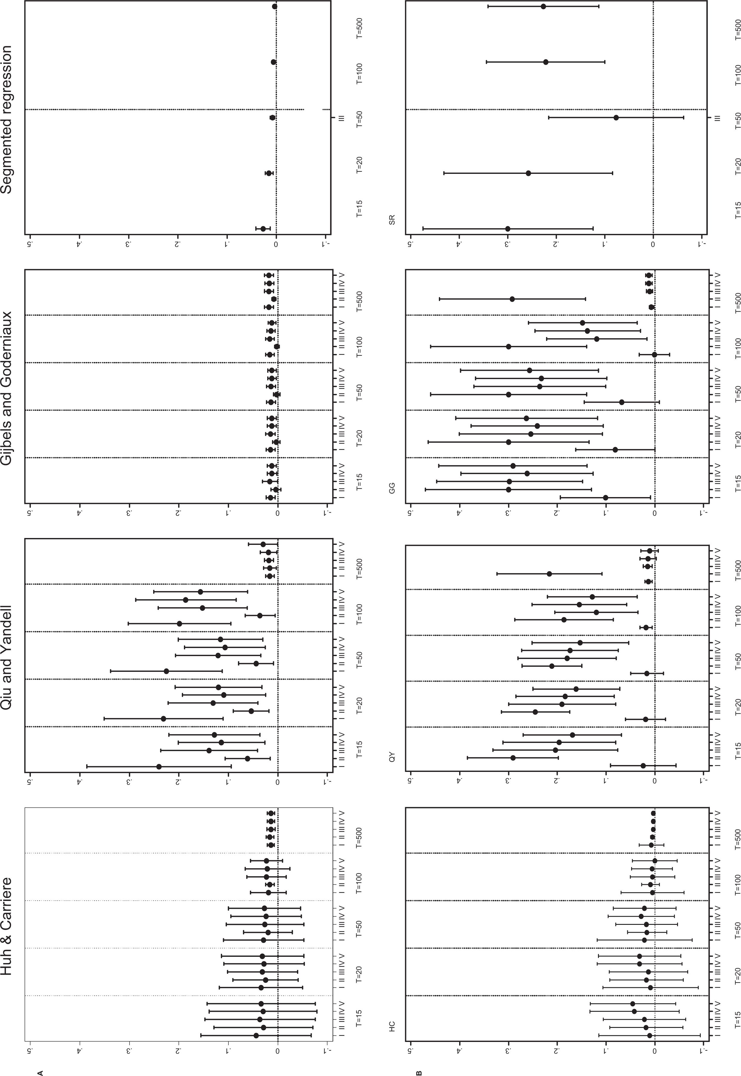
Absolute value of bias (dots) and root mean square error (RMSE; range plot) for the four change-point estimators Huh and Carierre (HC), Qiu and Yandell (QY), Gijbels and Goderniaux (GG), and segmented regression (SR) for regression functions (A) m ₂ and (B) m ₃ (Bias = absolute value of bias; RMSE = root mean square error; I = Plug-in bandwidth selection with polynomial of degree 1; II = Plug-in bandwidth selection with polynomial of degree 3; III = generalized cross-validation bandwidth selection; IV = bootstrap bandwidth selection with block length of 1; V = bootstrap bandwidth selection with block length of 5).

The GG estimator performed well for the regression setting m ₁ and m ₂, in contrast to the other assumed regression functions m ₃ and m ₄, where the bias was considerable. Regression functions m ₁, m ₂, m ₃, and m ₄ are characterized by a single kink at T = .5, whereas m ₃ and m ₄ additionally have a curvilinear shape with a maximum for T > .5. It is also notable that the first derivatives for m ₃ and m ₄ have a steep decrease for T > .5. The GG method estimated the maxima point of m ₃ and m ₄, although the first derivative is smooth at this interval. Already Gijbels and Goderniaux (2004b) has mentioned the estimation problems in derivatives with a steep increase and decrease, respectively. GG resulted in acceptable bias and RMSE estimates for large sets of design points.

There was no consistent pattern for good performance of QY. The plug-in estimator with polynomial of degree 3 acceptably worked in some scenarios, whereas it failed in other simulation settings.

The nonparametric estimators were also compared with the parametric SR method. It was not surprising that SR outperforms the nonparametric methods for regression functions m ₁ and m ₂ with its single kink at T = .5. SR failed in the more complex cases of m ₃ and m ₄ independent of the sample size T and is not suitable for estimation problems with nonlinear regression functions.

The estimated bandwidths for several selection methods are presented in Table 1 for λ = 10. The plug-in bandwidth estimators yielded bandwidths with slight variability and the bootstrap-estimated bandwidths were more variable, regardless of the chosen block length. The mean bandwidth of GCV was in between the plug-in with polynomial of degree 1 and plug-in with polynomial of degree 3. The bootstrap-estimated bandwidths were smaller than the plug-in with polynomial of degree 3 and were comparable to the GCV.

Table 1.

Mean and Standard Deviation of Estimated Bandwidths by Various Bandwidth Selection Methods and Sample Sizes T for Regression Functions m1, m2, m3, and m4, and λ = 10

		PI1		PI3		GCV		BB1		BB2			BB5		BB10
m	T	M	SD	M	SD	M	SD	M	SD	M		SD	M	SD	M		SD
m ₁	15	.266	.001	.352	.021	.340	.047	.263	.040		^_a		.278	.028		^_a
	20	.254	.001	.357	.019	.342	.037	.271	.030	.272		.024	.271	.031		^_b
	50	.213	.001	.336	.009	.245	.040	.243	.039	.242		.044	.242	.037	.251		.039
	100	.186	.001	.315	.006	.197	.029	.205	.030	.212		.037	.222	.045	.225		.043
	500	.136	.000	.267	.003	.136	.014	.144	.015	.140		.019	.141	.019	.146		.024
m ₂	15	.266	.001	.336	.023	.335	.040	.264	.040		^_a		.275	.032		^_a
	20	.254	.001	.336	.020	.334	.037	.266	.031	.270		.025	.265	.032		^_b
	50	.215	.001	.323	.014	.232	.039	.232	.040	.229		.037	.237	.040	.250		.040
	100	.187	.000	.308	.009	.184	.028	.199	.029	.203		.033	.217	.044	.227		.042
	500	.137	.000	.264	.003	.115	.013	.139	.017	.138		.017	.141	.018	.147		.029
m ₃	15	.194	.003	.306	.017	.319	.045	.247	.043		^_a		.269	0.35		^_a
	20	.180	.002	.305	.014	.319	.037	.260	.036	.264		.035	.264	.035		^_b
	50	.152	.001	.290	.010	.216	.034	.213	.036	.215		.037	.220	.039	.230		.043
	100	.133	.001	.276	.008	.178	.024	.183	.023	.185		.028	.188	.036	.212		.044
	500	.097	.000	.235	.003	.125	.012	.130	.013	.130		.015	.128	.015	.134		.023
m ₄	15	.196	.003	.305	.017	.325	.046	.254	.041		^_a		.272	.034		^_a
	20	.182	.002	.304	.015	.327	.038	.263	.034	.269		.031	.265	.033		^_b
	50	.152	.001	.288	.011	.226	.036	.218	.037	.216		.035	.225	.039	.232		.042
	100	.133	.001	.274	.008	.184	.025	.190	.023	.194		.026	.193	.037	.208		.040
	500	.097	.000	.233	.003	.129	.012	.135	.014	.134		.016	.135	.016	.135		.023

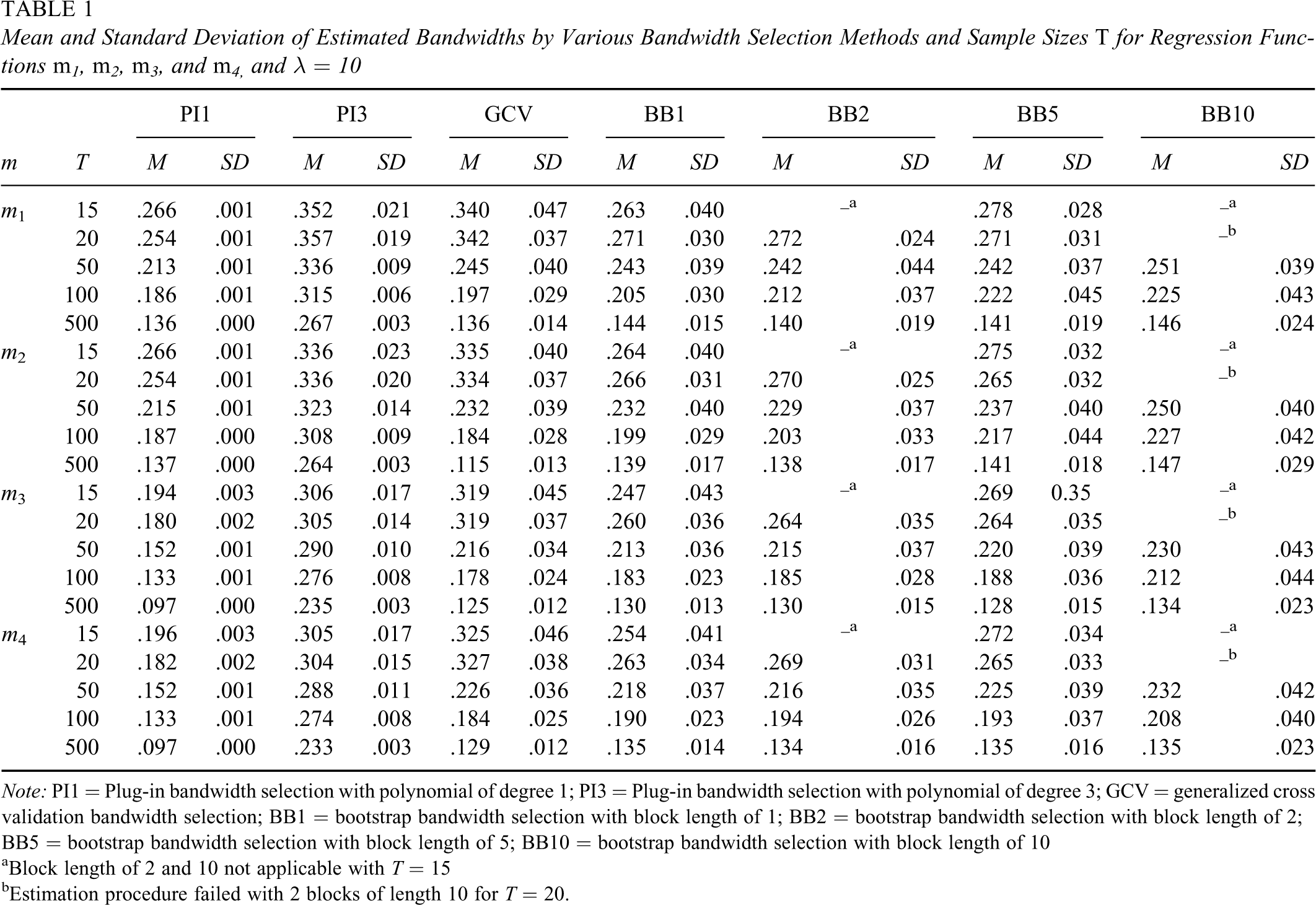
Note: PI1 = Plug-in bandwidth selection with polynomial of degree 1; PI3 = Plug-in bandwidth selection with polynomial of degree 3; GCV = generalized cross validation bandwidth selection; BB1 = bootstrap bandwidth selection with block length of 1; BB2 = bootstrap bandwidth selection with block length of 2; BB5 = bootstrap bandwidth selection with block length of 5; BB10 = bootstrap bandwidth selection with block length of 10

^aBlock length of 2 and 10 not applicable with T = 15

^bEstimation procedure failed with 2 blocks of length 10 for T = 20.

Summarizing the results of the Monte Carlo simulation study, the estimator of Huh and Carriere (Huh & Carriere, 2002) performed consistently by applying the plug-in bandwidth with polynomial of degree 3 and the block bootstrap (block length 10 in case of large sample sizes). The plug-in bandwidth method resulted in less variable estimates compared to the others.

Real Data Application: Performance-Related Anxiety

Musician Performance Data

The sample is comprised of five undergraduate music majors studying at a large university in the United States selected based on high levels of self-reported performance anxiety using the Performance Anxiety Scale (PAS; Nagel, Himle, & Papsdorf, 1981). The participants' mean PAS score was >1 SD above a previously established pretreatment mean (Nagel, Himle, & Papsdorf, 1989), thereby clearly representing individuals with a high propensity toward performance-related anxiety and impairment.

Participants recorded their data on a Palm m105 handheld computer and were instructed in their use before taking them home for a 1-week assessment period (Gloster & Klotsche, under review). Each participant recorded their responses to relevant performance anxiety questions on the handheld computer for 6 days prior to, the day of, and 1 day following a final performance examination in front of a jury of professors. The assessments were scheduled in an accelerating fashion such that the participants recorded 6 times (every 144 minutes) on Days 1 and 2, 7 times (every 120 minutes) on Days 3 through 6, 8 times on Day 7 (the performance day; every 90 minutes plus 10 minutes prior to and following the performance), and 5 times (every 144 minutes) on Day 8. The handheld computer signaled scheduled assessment via a loud set of beeps that repeated every 60 seconds until the participant responded. All data entered into the handheld computer were time stamped.

The data were collected via the handheld computer using the Worry–Anxious–Apprehension–Fear Scale (WAAF). The WAAF is based on the concept of a threat imminence continuum (Craske, 1999) and assesses five domains of anxiety believed to change with increasing threat: cognitions, mental images, emotions, self-perceived autonomic arousal, and avoidance. Each of the five domains consists of four questions. The WAAF total score is the sum of the 20 individual items.

Results

The values of the WAAF total score across time are presented in Figure 3 for the five participants and averaged across the five individuals (dots). The raw data were investigated for within-day patterns of anxiety. A consistent pattern of anxiety could not be found within a day across the study period. It is remarkable that the first measurement of the WAAF score was on a low level for the first 2 days compared to the other within-day measurements. The regression lines (solid line, Figure 3) were individually estimated for every music major by local polynomial regression as introduced in the method section applying the plug-in estimator of Ruppert (1997). The overall regression curve was calculated across the five music majors. The dashed vertical line represents the event of the performance examination in front of a jury of professors. The levels of the WAAF total score varied individually. A consistent pattern existed for the score across time as can be seen in Figure 3. The scores remained constant or decreased during the baseline period, likely due to familiarization with the study design, followed by an increase of the score before the performance examination and a strong decrease after the performance. The key question, however, is when exactly did the subjective assessments begin to increase above and beyond the baseline level. Identification of this point might suggest the point at which the impending performance becomes subjectively salient.

Figure 3.

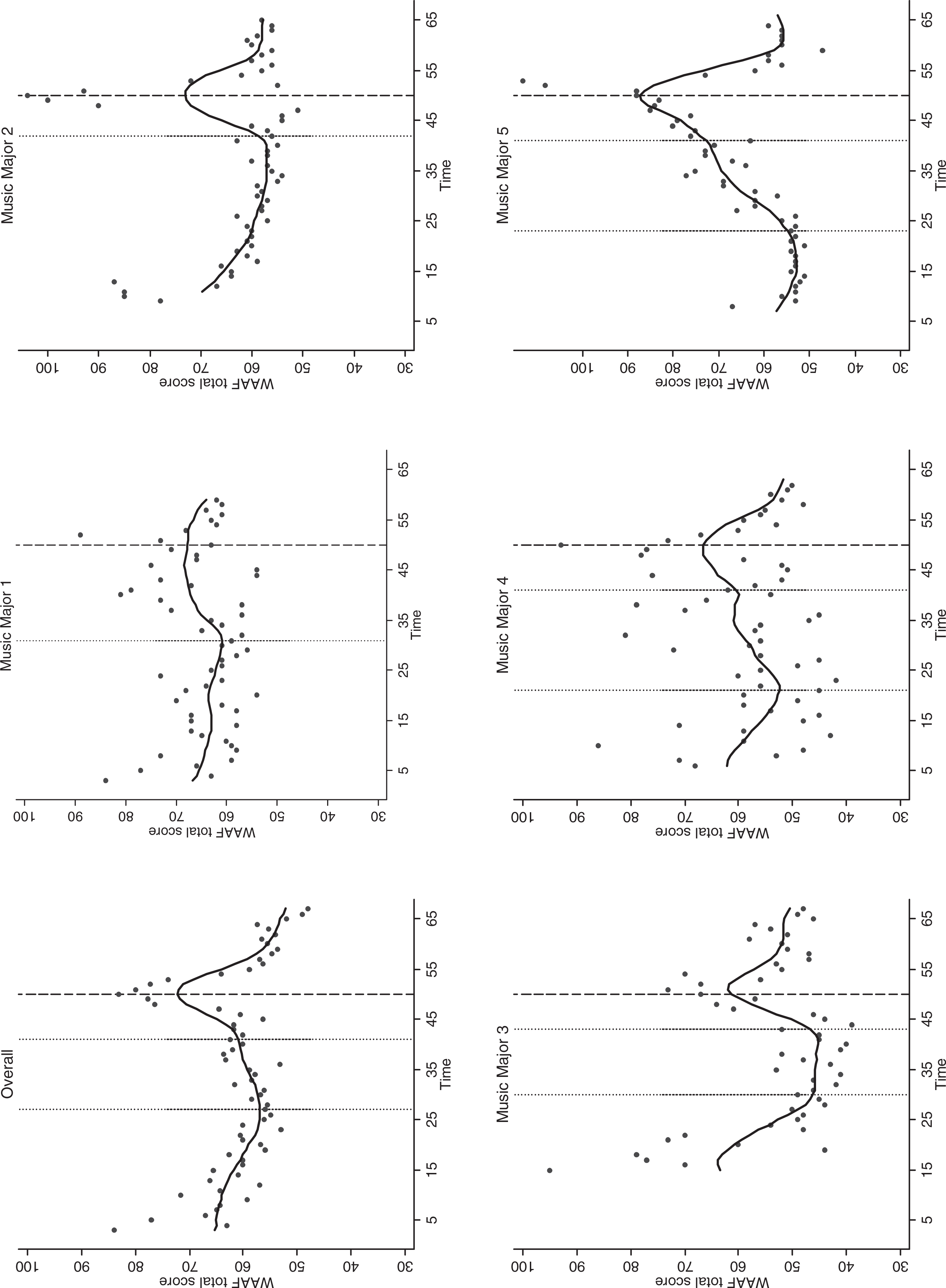
The individual raw Worry–Anxious–Apprehension–Fear Scale (WAAF) total scores across time for the five music majors and overall (dots: Individual values; solid line: Estimated nonparametric regression curve; dashed line: Event performance examination; dotted line: Estimated change-points).

The estimation method of Huh and Carriere (2002) was applied to estimate a meaningful change in the WAAF total score across time individually for the five music majors and across the data. The diagnostic function rhl − lhl (rhl of the first derivative minus lhl of the first derivative) is shown for the five participants and overall in Figure 4. The estimated change-point was given at the maximum of the diagnostic function rhl − lhl. It is supported by Figure 4 and the plot of the estimated regression lines in Figure 3 that there was one change-point for music major 1 ( ${\hat{θ}}_{1}$ = 31), music major 2 ( ${\hat{θ}}_{1}$ = 42), and two change-points for music major 3 ( ${\hat{θ}}_{1}$ = 30, ${\hat{θ}}_{2}$ = 43), music major 4 ( ${\hat{θ}}_{1}$ = 21, ${\hat{θ}}_{2}$ = 41), music major 5 ( ${\hat{θ}}_{1}$ = 23, ${\hat{θ}}_{2}$ = 41), and overall ( ${\hat{θ}}_{1}$ = 27, ${\hat{θ}}_{2}$ = 41). For example, the mean overall WAAF total score across time could be described by a decrease up to ${\hat{θ}}_{1}$ = 27, a flat increase up to ${\hat{θ}}_{2}$ = 41 followed by a steep increase up to the performance examination. The graph of rhl − lhl for music major 2 had a second local maxima at $\hat{θ}$ = 16. This local maxima was caused by the boundary problem, a less accurate estimated smoothed mean at the boundaries of the observed time interval as suggested by the comparison with the estimated regression line in Figure 4. A similar pattern existed for music major 3, but the maxima at ${\hat{θ}}_{1}$ = 30 was associated with a change in slope in contrast to music major 2.

Figure 4.

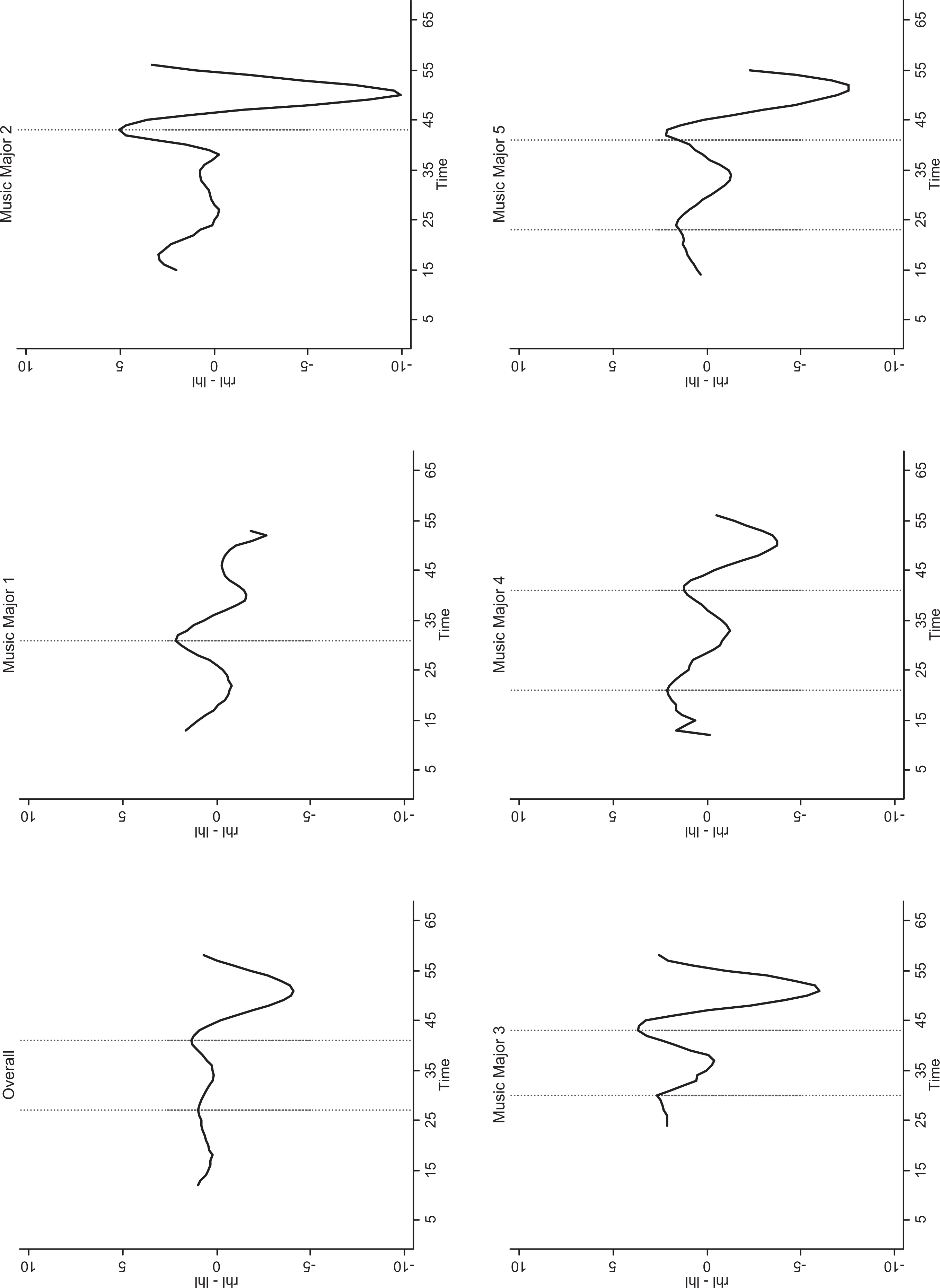
Diagnostic function right-hand limit minus left-hand limit of the first derivative in the estimation algorithm of Huh and Carriére (solid lines) and the selected change-points (vertical dotted lines).

SR analysis (Muggeo, 2003) was also applied to the musician performance data. Using multiple sets of starting values, a variety of possible estimates for θ were calculated (data not shown). The ambiguous results obtained when using segmented regression analysis could be explained by the large variance of the data and the nonlinear course of performance anxiety across time as indicated by Figure 3. The association between WAAF total score and time was modeled by a segmented linear function in the SR analysis.

Discussion

The identification of the change-point at which an observed outcome variable begins to meaningfully change above and beyond baseline fluctuations is an important research question in longitudinal data analysis. We considered a nonparametric modeling framework for estimating the change-point. Three possible exploratory estimation procedures were compared in a Monte Carlo simulation study. The estimator of Huh and Carriere (2002) yielded small biases and RMSE across many simulation settings. The estimator is based on a comparison of the lhl and rhl of the first derivative of the underlying unknown regression function. This procedure was applied to longitudinal data collected on performance anxiety of five musicians as they approach a performance. The estimation procedure HC yielded reasonable estimates of θ, whereas the parametric SR analyses failed. This method can be applied when a meaningful change-point is of interest in exploratory data analyses.

The measurements of anxiety levels (WAAF total score) were nested within day in our real data example. A systematic within-day pattern of performance anxiety has not been observed. It was not possible to account for the nested within-day observation in the discussed estimation framework, for example, as in random effect models. The dependent errors were taken into account by the bandwidth selection method.

It was shown in the simulation study that the estimator of Huh and Carierre performed well when only a small number of design points (T ≥ 15) are available. The estimator yielded ambiguous estimates, however, for design points less than 15 with results that were too variable. The estimator yielded also plausible results in the musician performance data used in this article. It is notable that the variance of the estimated regression functions was large (Participant 1: 47.0; Participant 2: 96.4; Participant 3: 55.4; Participant 4: 102.9; Participant 5: 74.1; and overall: 31.1). In contrast, the SR approach (Muggeo, 2003) resulted in implausible and variable estimates for the change-point depending on starting values for the estimation algorithm and the hypothesized functional pattern in for each segment.

Other methods on change-point detection in derivatives based on kernel smoothers exist. They include the work of Cheng and Raimondo (2008) in the time-series framework. They provided an estimator for the change-point θ based on the zero crossing technique. The change-point in the first derivative is estimated by applying a kernel approximation of the third derivative. The method resulted in good simulation results for large sets of design points (T = 1,000) while decreasing performance for T ≤ 200. One might expect a worse performance in the face of real data applications with limited design points of T < 25. The estimation algorithm of Cheng and Raimondo (2008) relies on an estimate of the third derivative. Higher-order derivatives are hard to estimate and large bandwidths are required for acceptable estimates (Qiu & Yandell, 1998). This fact provides a limitation in real data analyses with smaller sets of design points. The estimation problem of θ can also be addressed by spline smoothing (Barry, 2002) and the wavelet approximation (Wang, 1995) besides nonparametric regression analyses.

Loader (1999) compared the cross-validation criteria (Golub et al., 1979) with the plug-in estimator of Ruppert et al. (1995) in a regression model with independent and identically distributed errors. The results of an extensive simulation study yielded an ambiguous situation. The theoretical results could not be confirmed in simulated data about the superiority of plug-in-based methods over cross validation in respect to faster convergence and less variable estimates. Furthermore, a pilot estimator has to be calculated in the plug-in approach using estimates of higher-order derivatives assuming its smoothness. The failure of the assumption could yield inefficient estimates (Loader, 1999). The estimated bandwidths are smaller for the plug-in method applying a polynomial of first degree compared to GCV as reported in literature (Loader, 1999) in our Monte Carlo simulation study. The plug-in bandwidths get larger for higher-order polynomials. GCV and the bootstrapping procedure produce more variable estimates than the plug-in method. It is reported in literature (Loader, 1999) that the plug-in estimated bandwidths tend to oversmooth data with inflection points and curvature. This could be the reason for the superiority of the plug-in method applying a polynomial of third degree to the other bandwidth methods. Qiu and Yandell (1998) already pointed out that the derivatives are hard to estimate and large bandwidths are essential to get acceptable estimates.

The three estimation algorithms are based on local polynomial approximation of the outcome variable Y for design points T. The local polynomial approximation has benefits over both the kernel smoothed approaches of Nadayara and Watson (Nadaraya, 1964) and Gasser and Mueller (1979). (a) The boundary problem is addressed in local polynomial smoothing (Hastie & Loader, 1993). The boundary problem denotes the problem of a less accurate estimated smoothed mean at the boundaries of the observed time interval. (b) The estimated regression function m is improved when estimated in regions with few observations. (c) Local polynomial smoothing allows for an easy way to estimate the derivatives of the regression function m, which plays an important role in the estimation process of the change-point θ proposed in the nonparametric approach laid out in this article.

The large bandwidths represent a limitation of the framework modeling discussed here in the article. The first derivative is not estimated accurately at the boundaries of the considered time interval, although the boundary problem is addressed in local polynomial regression analyses (Hastie & Loader, 1993). The estimate of the lhl of the first derivative is based on only very few measurements at a time point at the beginning of the time interval, whereas the estimate of the rhl is based on the whole range of measurement points defined by the bandwidth. The fact results in artificial differences between the lhl and rhl of the first derivative at an observed time point close to the starting point and endpoint of the time interval.

Another limitation in real data analyses is the lack of statistical hypothesis testing, whether the observed discontinuity is statistically significant. Qiu and Yandell (1998) calculated a threshold if the estimated change-point is meaningful, but the corresponding estimator for θ did not perform well in our simulation study. It is recommended to plot the function rhl minus lhl of the first derivative in the method of Huh and Carriere (2002) in application to real data. The automatic estimation of the maximum of that function could yield false estimates because of the boundary problem discussed above.

Footnotes

Acknowledgments

The authors would like to thank the editor and the anonymous reviewer for their helpful suggestions what improved the clarity of this article.

References

Barry

(2002). A Bayesian analysis for derivative change points. Communications in Statistics-Theory and Methods, 31, 1335–1348.

Brown

L. D.

Low

M. G.

(1996). Asymptotic equivalence of nonparametric regression and white noise. Annals of Statistics, 24, 2384–2398.

Carpenter

Bithell

(2000). Bootstrap confidence intervals: When, which, what? A practical guide for medical statisticians. Statistics in Medicine, 19, 1141–1164.

Cheng

M. Y.

Raimondo

(2008). Kernel methods for optimal change-points estimation in derivatives. Journal of Computational and Graphical Statistics, 17, 56–75.

Chu

C. K.

Marron

J. S.

(1991). Comparison of two bandwidth selectors with dependent errors. Annals of Statistics, 19, 1906–1918.

Craske

M. G.

(1999). Anxiety disorders: Psychological approaches to theory and treatment. Boulder, CO: Westview Press

Efron

Tibshirani

R. J.

(1993). . In An introduction to the bootstrap (pp. –). London, England: Chapman and Hall.

Faraway

J. J.

Jhun

M. S.

(1990). Bootstrap choice of bandwidth for density estimation. Journal of the American Statistical Association, 85, 1119–1122.

Gasser

Mueller

H. G.

(1979). Kernel estimation of regression functions. In Smoothing Techniques for Curve Estimation: Proceedings of a Workshop Held in Heidelberg, April 2–4, 1979 (pp. 23–68). Berlin: Springer-Verlag.

10.

Gasser

Mueller

H. G.

Mammitzsch

(1985). Kernels for nonparametric curve estimation. Journal of the Royal Statistical Society Series B–Methodological, 47, 238–252.

11.

Gijbels

Goderniaux

A. C.

(2004a). Bandwidth selection for change-point estimation in nonparametric regression. Technometrics, 46, 76–86.

12.

Gijbels

Goderniaux

A. C.

(2004b). Data-driven discontinuity detection in derivatives of a regression function. Communications in Statistics-Theory and Methods, 33, 851–871.

13.

Gloster

A. T.

Richard

D. C. S.

Himle

Koch

Anson

Lokers

Thornton

(2008). Accuracy of retrospective memory and covariation estimation in patients with obsessive-compulsive disorder. Behaviour Research and Therapy, 46, 642–655.

14.

Golub

G. H.

Heath

Wahba

(1979). Generalized cross-validation as a method for choosing a good ridge parameter. Technometrics, 21, 215–223.

15.

Haerdle

(1990). . In Applied nonparametric regression (pp. –). Cambridge, UK: Cambridge University Press.

16.

Hall

Lahiri

S. N.

Polzehl

(1995). On bandwidth choice in nonparametric regression with both short- and long-range dependent errors. Annals of Statistics, 23, 1921–1936.

17.

Hartmann

D. P.

Gottman

J. M.

Jones

R. R.

Gardner

Kazdin

A. E.

Vaught

R. S.

(1980). Interrupted time-series analysis and its application to behavioral-data. Journal of Applied Behavior Analysis, 13, 543–559.

18.

Hastie

Loader

(1993). Local regression—Automatic kernel carpentry. Statistical Science, 8, 120–129.

19.

Hidalgo

(1997). Non-parametric estimation with strongly dependent multivariate time series. Journal of Time Series Analysis, 18, 95–122.

20.

Huh

Carriere

K. C.

(2002). Estimation of regression functions with a discontinuity in a derivative with local polynomial fits. Statistics & Probability Letters, 56, 329–343.

21.

Kashdan

T. B.

Steger

M. F.

(2006). Expanding the topography of social anxiety—An experience-sampling assessment of positive emotions, positive events, and emotion suppression. Psychological Science, 17, 120–128.

22.

Loader

C. R.

(1999). Bandwidth selection: Classical or plug-in?. Annals of Statistics, 27, 415–438.

23.

Morgan

O. W.

Griffiths

Majeed

(2007). Interrupted time-series analysis of regulations to reduce paracetamol (acetaminophen) poisoning. PLoS Medicine, 4, 654–659.

24.

Mueller

H.-G.

Stadtmueller

(1999). Discontinuous versus smooth regression. Annals of Statistics, 27, 299–337.

25.

Muggeo

V. M. R.

(2003). Estimating regression models with unknown break-points. Statistics in Medicine, 22, 3055–3071.

26.

Mueller

H. G.

(1992). Change-points in nonparametric regression-analysis. Annals of Statistics, 20, 737–761.

27.

Mueller

H. G.

Song

K. S.

(1997). Two-stage change-point estimators in smooth regression models. Statistics & Probability Letters, 34, 323–335.

28.

Nadaraya

E. A.

(1964). On estimating regression. Theory of Probability and Its Applications, 9, 141–142.

29.

Nagel

J. J.

Himle

D. P.

Papsdorf

J. D.

(1981). Coping with performance anxiety. NATS Bulletin, 37, 26–33

30.

Nagel

J. J.

Himle

D. P.

Papsdorf

J. D.

(1989). Cognitive-behavioral treatment of musical performance anxiety. Psychology of Music, 17, 12–21.

31.

Opsomer

Wang

Y. D.

Yang

Y. H.

(2001). Nonparametric regression with correlated errors. Statistical Science, 16, 134–153.

32.

Qiu

P. H.

Yandell

(1998). A local polynomial jump-detection algorithm in nonparametric regression. Technometrics, 40, 141–152.

33.

Ruppert

(1997). Empirical-bias bandwidths for local polynomial nonparametric regression and density estimation. Journal of the American Statistical Association, 92, 1049–1062.

34.

Ruppert

Sheather

S. J.

Wand

M. P.

(1995). An effective bandwidth selector for local least squares regression. Journal of the American Statistical Association, 90, 1257–1270.

35.

Shiffman

Stone

A. A.

Hufford

M. R.

(2008). Ecological momentary assessment. Annual Review of Clinical Psychology, 4, 1–32.

36.

Stone

A. A.

Schwartz

J. E.

Broderick

J. E.

Shiffman

S. S.

(2005). Variability of momentary pain predicts recall of weekly pain: A consequence of the peak (or salience) memory heuristic. Personality and Social Psychology Bulletin, 31, 1340–1346.

37.

Stone

A. A.

Shiffman

(2002). Capturing momentary, self-report data: A proposal for reporting guidelines. Annals of Behavioral Medicine, 24, 236–243.

38.

Taylor

C. C.

(1989). Bootstrap choice of smoothing parameter in kernel density estimation. Biometrika, 76, 705–712.

39.

Wagner

A. K.

Soumerai

S. B.

Zhang

Ross-Degnan

(2002). Segmented regression analysis of interrupted time series studies in medication use research. Journal of Clinical Pharmacy and Therapeutics, 27, 299–309.

40.

Wang

Y. Z.

(1995). Jump and sharp cusp detection by wavelets. Biometrika, 82, 385–397.

41.

Yang

Y. H.

(2001). Nonparametric regression with dependent errors. Bernoulli, 7, 633–655.