
Abstract
Parametric methods, such as autoregressive models or latent growth modeling, are usually inflexible to model the dependence and nonlinear effects among the changes of latent traits whenever the time gap is irregular and the recorded time points are individually varying. Often in practice, the growth trend of latent traits is subject to certain monotone and smooth conditions. To incorporate such conditions and to alleviate the strong parametric assumption on regressing latent trajectories, a flexible nonparametric prior has been introduced to model the dynamic changes of latent traits for item response theory models over the study period. Suitable Bayesian computation schemes are developed for such analysis of the longitudinal and dichotomous item responses. Simulation studies and a real data example from educational testing have been used to illustrate our proposed methods.
Keywords
1. Introduction
Longitudinal studies play a prominent role in investigating temporal changes in a construct of interest, which are often referred to as growth curve analysis in social and behavior science. The advent of computerized testing and online rating brings an entirely new way for social and behavior researchers to collect longitudinal data. Test takers have much more freedom to choose their test time than before. Then, the responses collected are often observed at variable and irregular time points across individuals. The randomness of responses may further create sparsity in certain period, such as in the summer or winter holidays.
Traditionally, there are two models of wide usage for studying individual changes. One is called latent growth curve modeling (Bollen & Curran, 2006) and the other is multilevel modeling or hierarchical linear modeling (Raudenbush & Bryk, 2002). However, when outcomes are observed at individually varying and irregularly spaced time points, the inferences from these two traditional models for studying individual changes may become problematic due to the uneasy adjustment of parametric structures in the models (Geiser, Bishop, Lockhart, Shiffman, & Grenard, 2013). For instance, their analysis typically required the same time span of the study and the same testing points for all examiners. Furthermore, for computerized testing/survey in education, the manifest responses are usually dichotomous, ordinal, or nominal, while latent traits needed to be inferred are often continuous. These make the inference even more difficult because of the information loss in the discretization procedure of the underlying latent variables. In this article, we mainly focus on the extension of classic item response theory (IRT) model framework to model longitudinal dichotomous data collected at irregular and variable time points.
1.1. Review of Relevant Literature
There are two major approaches, that is, the multidimensional and multilevel approach, available in the current literature of IRT models for the analysis of longitudinal data. First, for the multidimensional approach, a multidimensional IRT model is used to represent the change of an ability as an initial ability and one or more modified ability in unidimensional or multidimensional tests (Cho, Athay, & Preacher, 2013; Embretson, 1991; te Marvelde, Glas, Landeghem, & Damme, 2006). However, this approach allows little variation of items on different occasions, and it often requires the individuals to take the same tests. These drawbacks prevent us from extending their methods to analyze a time series of computerized testing data.
Second, for the multilevel approach, the first level is often assumed to follow a classic IRT model, while in the higher level, there are two common ideas to model the growth. One idea is to assume the growth of a latent trait be parametric function of time, such as a linear or polynomial regression of the time variable with fixed or random coefficients. This idea is a variation of the latent growth curve modeling in the analysis of binary/categorical longitudinal data (Albers, Does, Imbos, & Janssen, 1989; Hsieh, von Eye, Maier, Hsieh, & Chen, 2013; Johnson & Raudenbush, 2006; Tan, Ambergen, Does, & Imbos, 1999; Verhagen & Fox, 2012). Another idea is to employ Markov chain models, where the changes of a latent trait over time are assumed to be dependent on its previous value or status (Bartolucci, Pennoni, & Vittadini, 2011; Kim & Camilli, 2014; Martin & Quinn, 2002; Park, 2011). However, there are many instances in which neither of two ideas would be enough to describe the growth (Bollen & Curran, 2004). One of such instances is computerized testing, especially when the time lapses between tests are unequally spaced across individuals as well as within individuals.
To tackle the challenges in computerized testing for modeling the growth of latent traits, Wang, Berger, and Burdick (2013) proposed a dynamic model by combining the ideas of parametric functions of time as well as Markov chain models to describe the growth. They imbedded IRT models into a new class of state space models for analyzing longitudinal data located at individually varying and irregularly spaced time points. Nevertheless, assuming a particular functional relationship for the growth in general is restrictive and usually difficult to justify. Instead, a nonparametric model could be much more flexible to describe changes of latent traits and avoid the errors of model misspecification.
As further investigation of the results shown in Wang et al. (2013), we found the trajectory of one’s reading ability grows more quickly in the initial period but slows down when it approaches maturation. Overall, the ability exhibits an increasing trend but often has a flat region at the end. Such discovery of the shape for the growth trajectory is consistent with prior beliefs and experiences from practitioners. In social or behavior science, prior knowledge about the shape of the trajectory, such as monotonicity, convexity, or concavity, may be available ahead of the analysis to aid in the modeling process and enhance interpretability. This calls our attention to incorporate shape constraints as a prior information to nonparametric modeling. It is expected that the usage of shape information may improve the efficiency and accuracy of the nonparametric estimates.
From the Bayesian perspective, nonparametric regression with monotonicity constraints has already been considered in the literature. For instance, Gelfand and Kuo (1991) used an ordered Dirichlet process prior to impose the monotone constraint. Neelon and Dunson (2004) imposed a piecewise linear regression, with an autoregressive prior for the parameters of basis functions. Shively, Sager, and Walker (2009) as well as Brezger and Steiner (2012) implemented restricted splines to ensure monotonicity. McKay Curtis and Ghosh (2011) used Bernstein polynomials with restrictions on parameter space, while Choi, Kim, and Jo (2016) extended this idea by allowing incorporation of uncertainty of the constraints through the prior. Lin and Dunson (2014) proposed Gaussian process projection to perform shape-constrained inference and applied the method to multivariate surface estimation. Wang and Berger (2016) imposed the constraints on the derivative process of the original Gaussian process to estimate shape-constrained functions.
However, typical nonparametric models are often less interpretable. In this article, enlightened by the idea of Bornkamp and Ickstadt (2009), we imbed a flexible Bayesian nonparametric monotone regression of latent traits into the IRT models with easy interpretation. The monotone regression can be written as the sum of two parts: (1) an intercept parameter (interpretable as one’s initial ability) and (2) the product of a scale parameter (interpretable as the maximum ability that one can grow during the study period) with a continuous function of the time variable (which is monotonically increasing over the study period and can easily capture the plateaus effect of one’s ability at the end). Another advantage of our proposed approach is that the parameters for the underlying base functions which constitute the monotone function do not have constraints on the domain of parameter space. Lacking of constraints on the parameter space could make the model more flexible and reduce computational burden. Additionally, the base functions themselves can be directly learned from the data.
1.2. EdSphere Test Bed Application
We will apply our proposed method to the EdSphere data set provided by Highroad Learning Company. EdSphere is a personalized literacy learning platform that continuously collects data about student performance and strategic behaviors each time when he or she reads an article. During a typical reading test, a student selects from a system-generated list of articles having the test difficulty level in a range targeted to the current estimate of the student’s ability. Then, for the selected article, a subset of words from the article is eligible to be clozed, that is, removed and replaced by a blank. The computer, following a prescribed protocol, randomly selects a sample of the eligible words to be clozed and presents the article to the student with these words clozed. The question items produced by this procedure are randomized items. They are single-use items generated at the time of an encounter between a student and an article. If another student selects the same article to read, a new set of clozed words is selected. As a consequence, the occurrence of individual items among students is highly improbable, so obtaining empirical estimates of item parameters is not feasible.
The difficulty levels of the items in the reading test are provided by MetaMetrics using proprietary data and methods. The ensemble mean and the variance of difficulty level for the items in a test are known due to the test design of EdSphere learning platform.
Currently, the EdSphere data set consists of 16,949 students from a school district in Mississippi, who participated over 5 years (2007–2011) in EdSphere learning platform. A snapshot of the data sets is included in Table B1 in the online version of the article. The students were in different grades and could enter and leave the program at different times. They were free to take tests on different days and had different time lapses between tests. This design yields longitudinal observations located at individually varying and irregularly spaced time points and suggests that we need to model the changes of latent traits with a dynamic structure. Further, in the spirit of EdSphere test design, we could imagine the factors, such as overall comprehension, emotional status, and others, would exist and undermine the local independence assumption of IRT models as mentioned in Wang et al. (2013). Therefore, we aim to extend the classic IRT models to accommodate the modern computerized (adaptive) testing (not merely EdSphere data sets), which have the described distinctive features, that is, randomized items, longitudinal observations, and local dependence.
2. Nonparametric Monotone Regression
In this article, we keep the discussion focused on the one-parameter IRT model that links latent ability and item difficulty to the correctness of each item. The idea could be similarly implemented on two-parameter/three-parameter IRT models or other continuous, ordinal, and nominal latent variable models. In the classic one-parameter IRT model, the latent ability of each individual and the difficulty level for each item are the two key components and often they assume to be static. But in the EdSphere data set, the item responses are longitudinal, and thus, the latent ability of individuals and item difficulty levels are both varying with time. In addition, each test taker is allowed to take tests at any time they wish in the computerized testing. Moreover, they can take more than one exams per day. Therefore, following the discussion of Wang et al. (2013), we need to extend the classic one-parameter IRT model as below.
The proposed shape-constrained IRT model involves two levels, that is,


In the first level, Equation 1 extends the classic one-parameter IRT models to the scenario of computerized testing, where

where
In the second level (Equation 2),
We will utilize the idea of Bornkamp and Ickstadt (2009) to model the unknown latent trajectory

where

where we model
In Equation 5, proper choice of the base distribution function
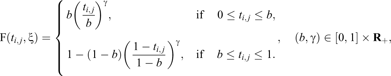
which has two key parameters
We illustrate several examples of TSP functions in Figure 1. From Figure 1, we can see that γ controls the steepness of the curve. When γ is small, the pace of increasing is comparatively slow, and when γ becomes larger, the increasing trend becomes steeper. The parameter b is the unique mode of TSP function when

Illustration of several two-sided power functions with different γ and b values.
3. Bayesian Computation Scheme
The hierarchical model of Equations 1 and 2 can accommodate the complex structure of computerized testing (e.g., EdSphere data sets), and it also allows the incorporation of prior information. However, because of the complexity of the model considered, we have to resort to Markov chain Monte Carlo (MCMC) computational techniques for the analysis. A by-product of Bayesian inference is that all uncertainties in all quantities are combined in the overall assessment of inferential uncertainty.
3.1. Prior Specification and Posterior Distribution
Before starting the Bayesian inference, first, we have to specify the prior distributions of unknowns in the model. For parameters ϕ,
According to Lemma 1 in Bornkamp and Ickstadt (2009), the prior distributions of
Using the priors specified above, we can derive the posteriors of unknowns in the proposed model as shown in Equation 8 of online Appendix A. We can show this posterior is proper (see details in online Appendix A). Then, the statistical inferences based on the sampling from this posterior is legitimate. To facilitate the computation for the posterior of unknowns, we implement the idea of data augmentation (Albert & Chib, 1993) by introducing a latent variable

with
Let us denote
Similarly, we use bold notations
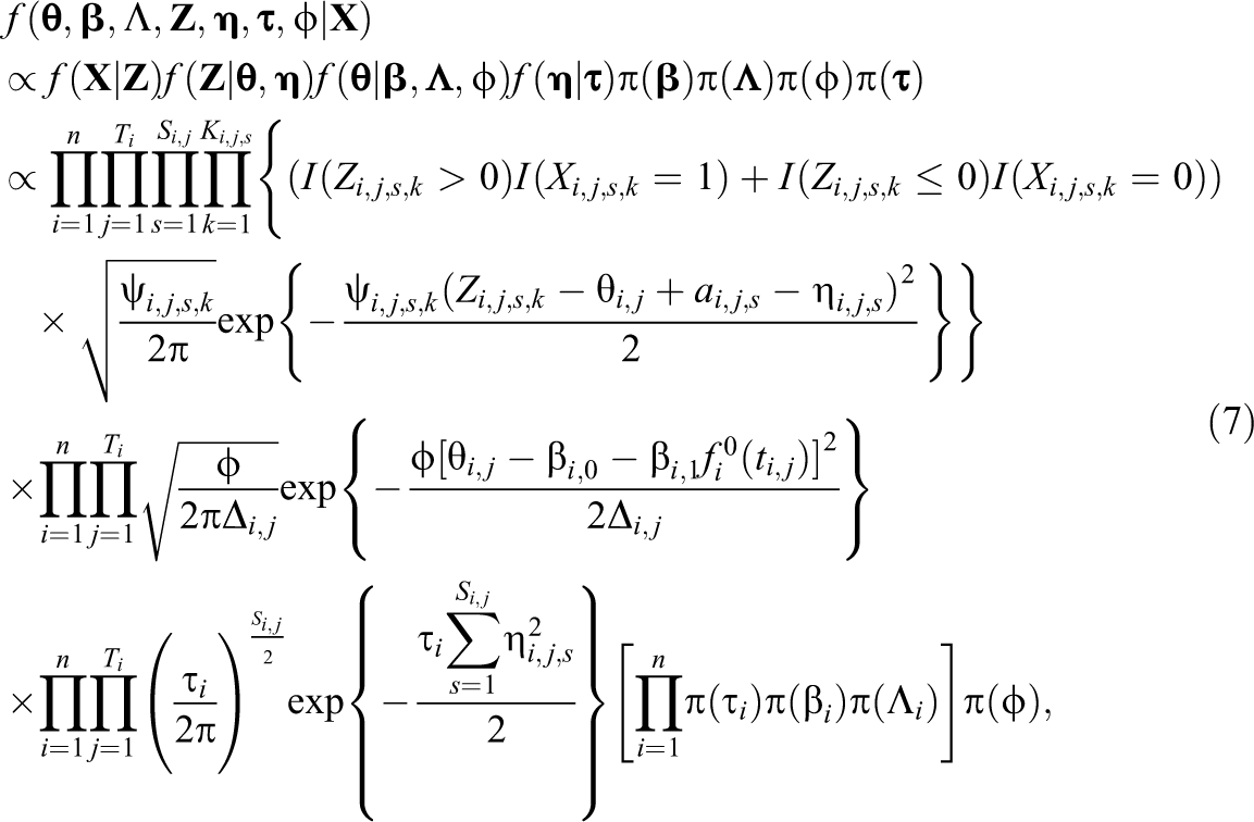
where
3.2. The MCMC Sampling Schemes
The key part in developing MCMC algorithm to draw samples from the joint posterior distribution (Equation 7) is to estimate the latent trajectory
Sample
Sample
Sample
Sample
Sample
Sample
Sample
The details of each sampling step are described in online Appendix A. The MCMC sampling loops through Steps 1 through 7 and repeats until the MCMC is converged. The initial values (i.e., when
Then, statistical inferences are made straightforward from the MCMC samples. For example, an estimate and 95% credible interval (CI) for the latent trajectory of one’s ability
4. Simulation Examples
To validate the inference procedure of MCMC schemes and show the success of using monotone shape constraints in the nonparametric modeling, two simulation studies are conducted. For the first simulated example, we know the true underlying curve
4.1. An Example Using the Mixture of TSP Functions as the Latent Trajectory
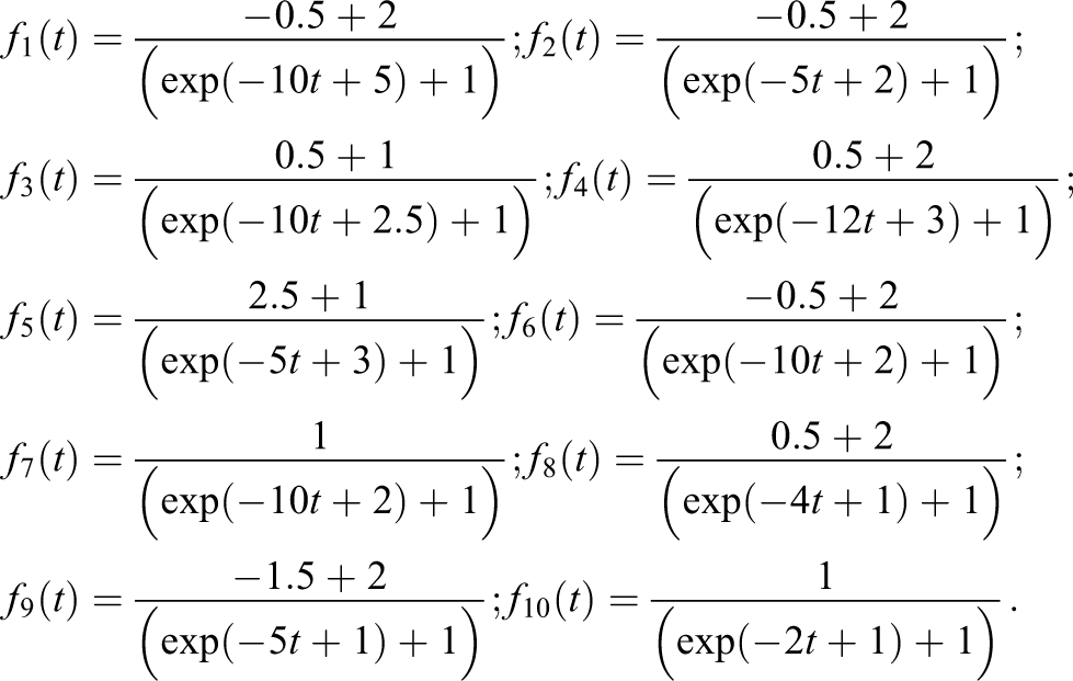
In this section, we apply our proposed method to a simulated data set that uses the mixture of TSP functions as the true latent trajectory. We consider 10 test takers, that is,
We set the true values for model parameters as below:
Simulated Parameters for Each Individual of Two-Sided Power Functions
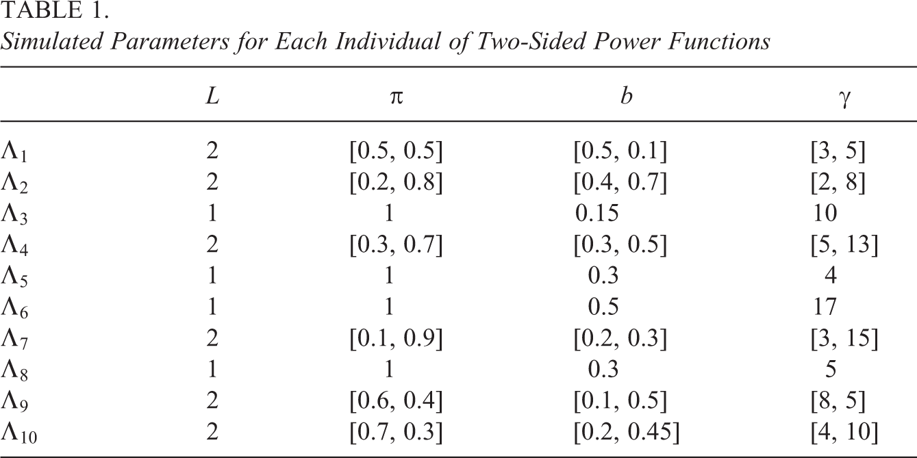
We use the prior specified in Section 3.1 for the unknown parameters of the proposed model. Particularly, for this simulated example, we use a zero-truncated Poisson for each Li
with
Model fitting is done with the MCMC algorithm described in the Section 3.2, based on 50,000 iterations in total. The first 10,000 samples are burned in, and only every 20th value is taken for our inference as to reduce dependence. After this burn-in process, the mixing of MCMC samples looks pretty good, and the trace plots of MCMC samples of parameters are convergent.
In Figure 2, we display results of 4 represented individuals among the 10 simulated individuals in the example. Those four individuals have noticeable differences in the shape of their corresponding trajectories. The growth curve for the first subject is steadily increasing without obvious transition. While for the second individual in Figure 2, he or she has obvious turning points. He or she grows slowly during the initial period, then rapidly grows in the middle and reaches the plateaus in the end. For third and sixth subjects in Figure 2, they have similar phenomena as the second individual but with different lengths of the three stages in the study.
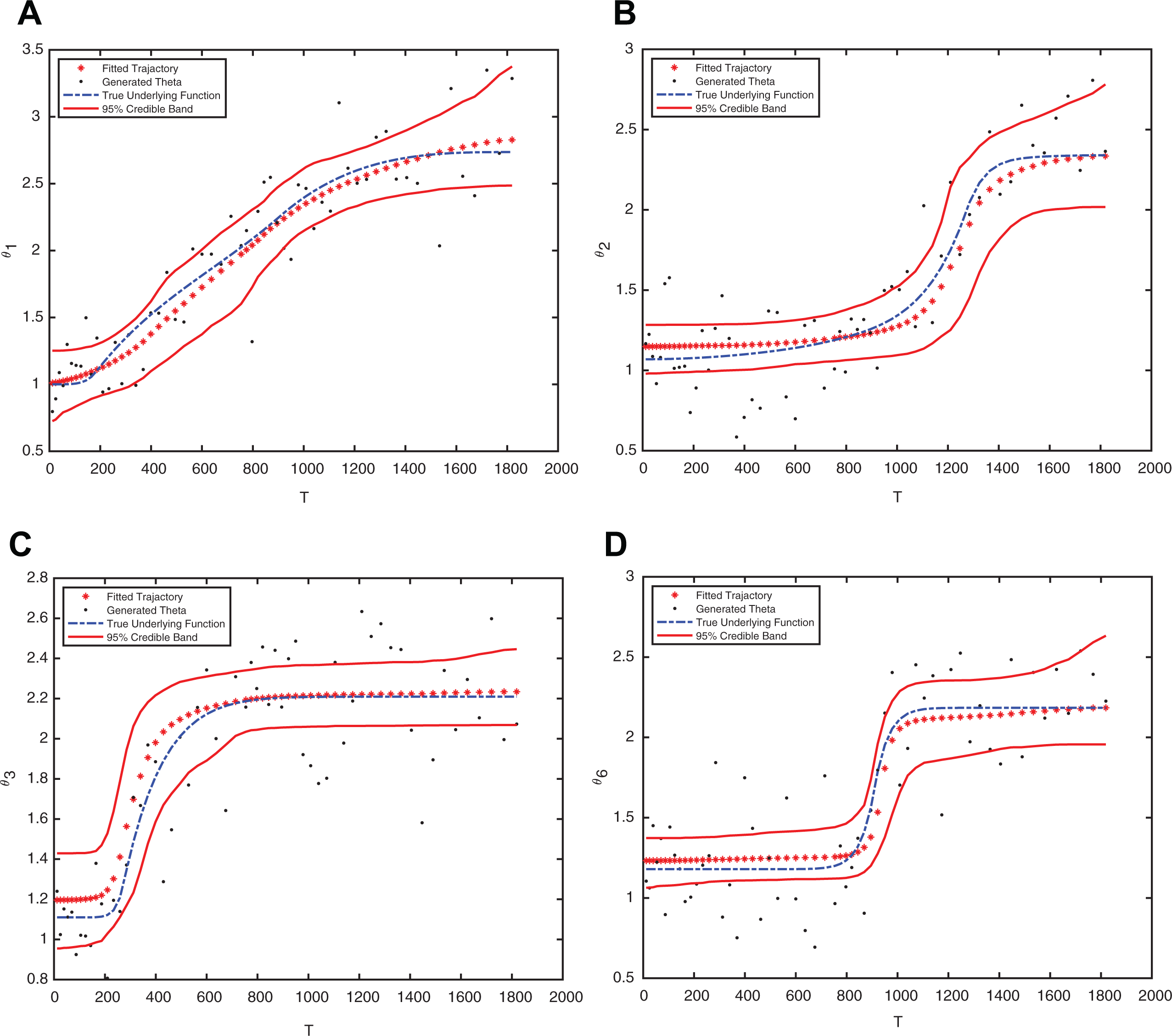
The estimation of latent trajectories for the first, second, third, and sixth subjects. (A) First individual. (B) Second individual. (C) Third individual. (D) Sixth individual.
In each subfigure of Figure 2, the dash line represents the true underlying function
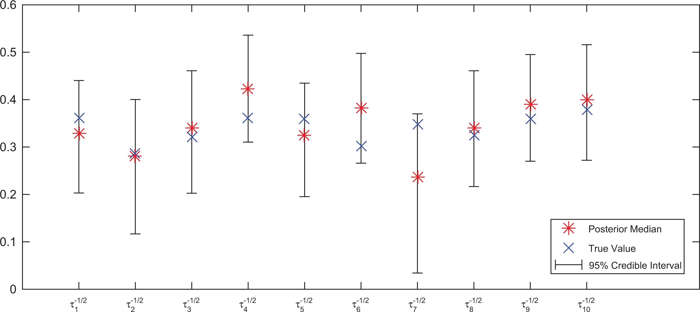
We also calculate the posterior estimates of all other unknowns. The posterior median of
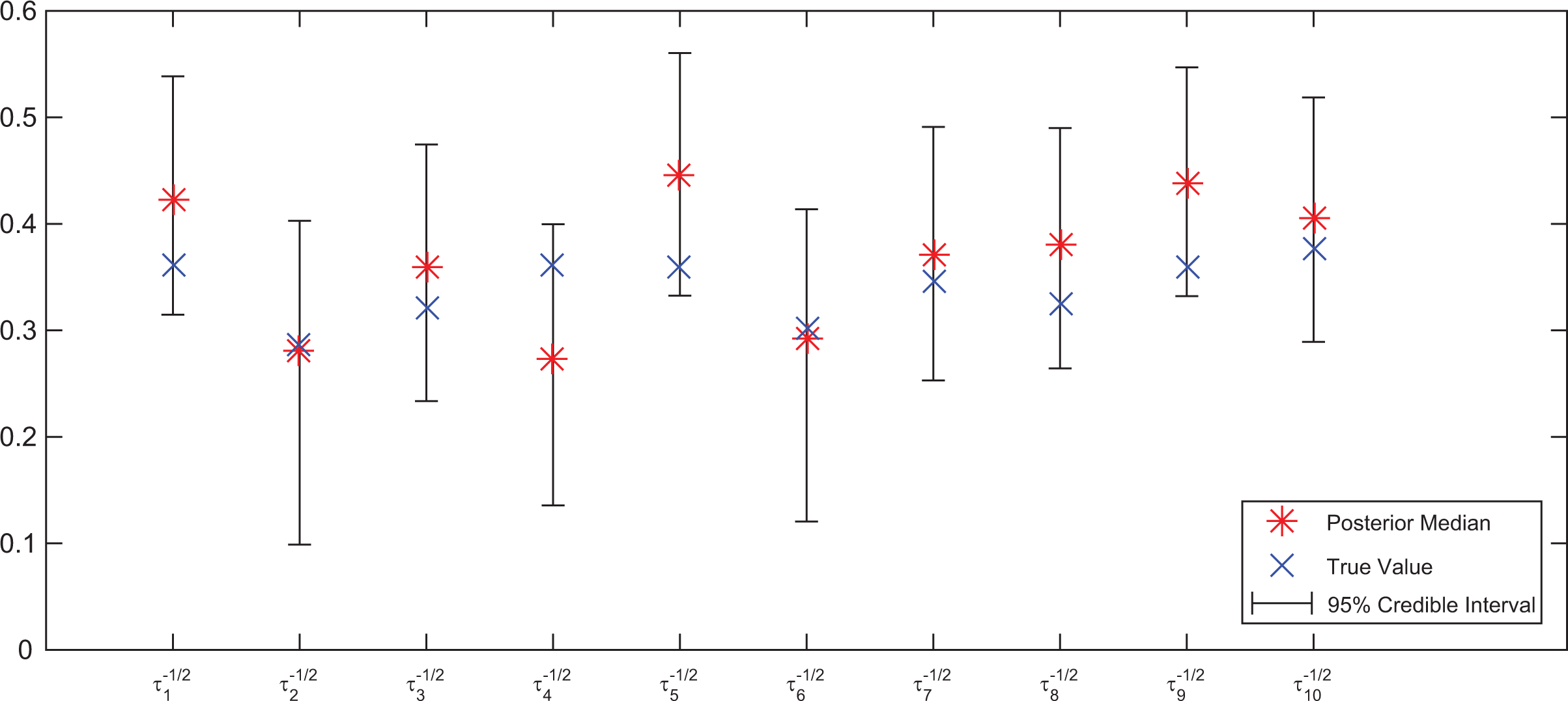
Posterior median and 95% CIs of
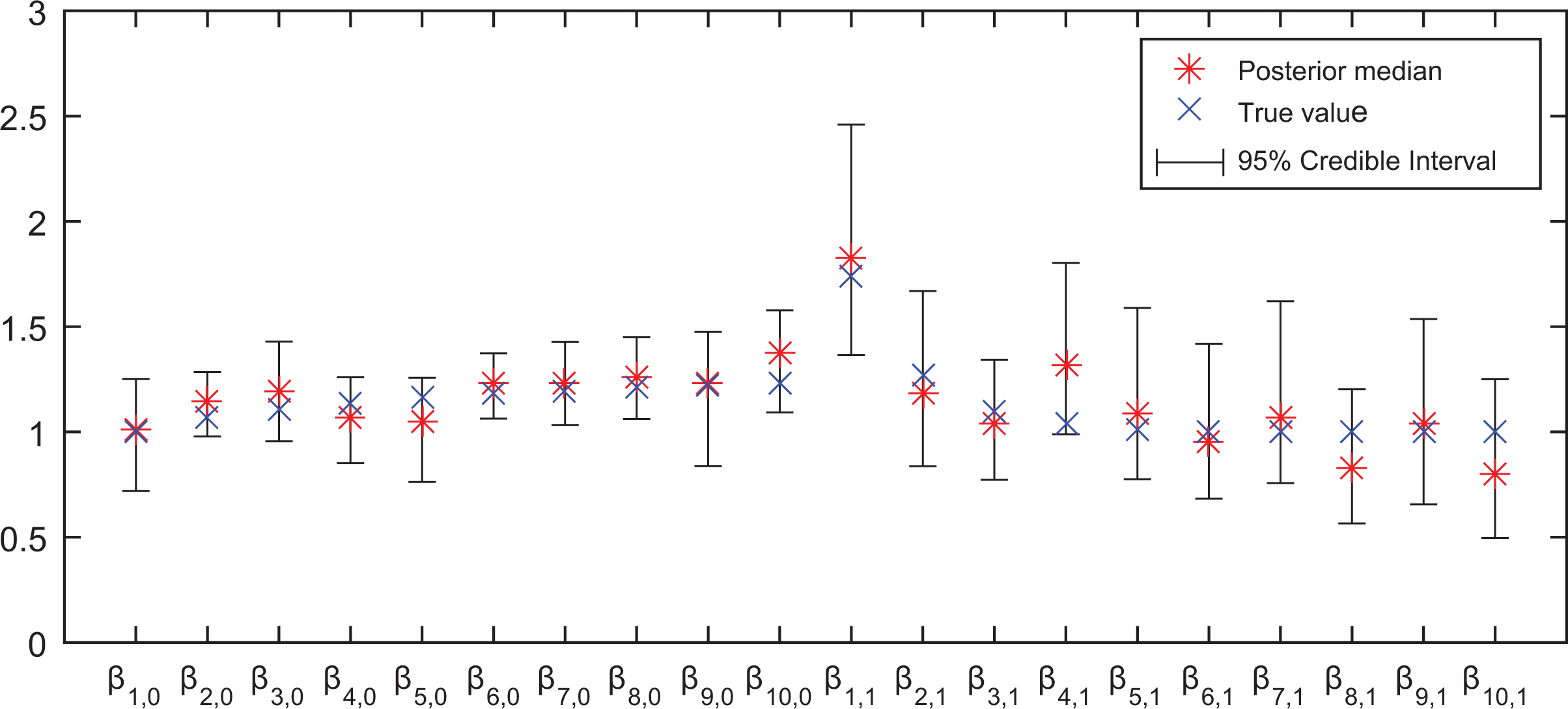
The results of posterior median and 95% CIs of
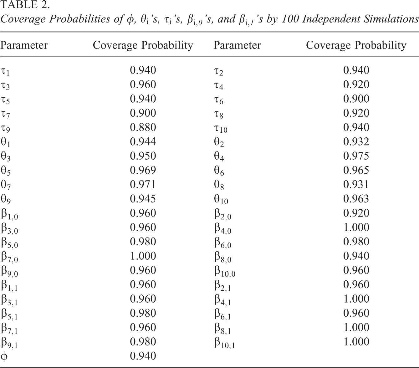
To take account of randomness in the simulations, another 100 independent data sets are simulated to check frequentist coverage probabilities, with same parameter setup but different random seeds. For each data set, we also run the MCMC sampling for 50,000 iterations with the first 10,000 samples being burned in. In addition, the MCMC chains are thinned by only using every 20th sample. The results are shown in Table 2. We can see that the coverage probabilities of the 95% CIs of all model parameters including the truth are equal or very close to the nominal level 95%. Thus, while the inferential method is Bayesian, it seems to yield sets that have good frequentist coverage.
Coverage Probabilities of ϕ,
4.2. An Example of the Logistic Curve as the Latent Trajectory
In this section, we apply our proposed method to some non-TSP-based true latent trajectories. The setup is the same as the previous simulation except the true trajectories
The motivation for using logistic curves as the true latent trajectories in the simulation is that the logistic curves have been widely applied in the growth curve analysis. Similarly, our model fitting is done based on 200,000 iterations in total. The first 40,000 samples are burned in, and every 20th value of MCMC samples is taken to reduce the dependence of samples. We use a zero-truncated Poisson for each Li
with
Figure 5 displays the results of four selected individuals, where the dash lines represent the truth of the underlying growth curve, the bullet dots are simulated values of

The estimation of latent trajectories for the fourth, sixth, seventh, and eighth subjects. (A) Second individual. (B) Fourth individual. (C) Sixth individual. (D) Eighth individual.
In addition, we calculate the posterior estimates of all other unknowns. The posterior median of
Posterior median and 95% CIs of

Posterior median and 95% CIs of
5. Application to EdSphere Data
Since our approach has been successfully applied to estimate the trend of
The prior specification is the same as the aforementioned simulation examples except we use a zero-truncated Poisson prior for each Li
with
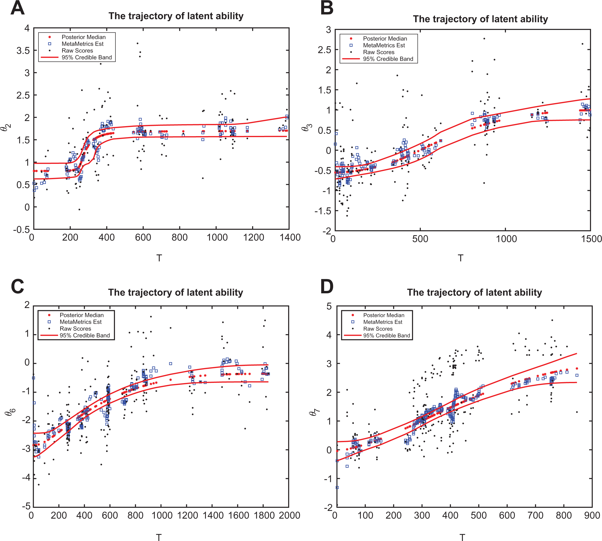
The estimation of latent trajectories for the second, third, sixth, and seventh subjects. (A) Second individual. (B) Third individual. (C) Sixth individual. (D) Seventh individual.
We have run in total 500,000 iterations and burn in the first one fifth of the samples, and to reduce dependence of MCMC samples, we have taken only every 20th value of MCMC samples. We have checked the trace plots of model parameters to access the convergence for MCMC samples, and we found a good mixing is observed after our burn-in and thinning process. Figure 8 shows the estimated trajectory of four individuals, which represent four types of growth curves we typically observed from the data.
In Figure 8, from our proposed method, the star dotted lines denote the corresponding 95% credible band of one’s latent trajectory, the square dots represent the estimated trajectory used in current EdSphere learning platform (where they assume AR(1) model for
Noticeably, in Figure 8, the latent growth curve of the second individual (i.e., see Figure 8[A]), a six-grader, increases sharply at about the 300th day and reaches the plateau before the 450th day, while the sixth individual (in Figure 8[C]) experiences a moderate growth during most of the time before stabilizing by the end of the study. For the third and the seventh students in Figure 8(B) and 8(D), respectively, they both are in Grade 2 and have a similar type of steadily increasing shape of the growth over the entire study period. However, seen from Figure 8, the growth rate (or learning speed) of the seventh individual is much faster than that of the third individual. Since the study period of seventh individual is much shorter than that of the third individual, clearly, we can also compare the estimation of posterior median as well as the corresponding 95% CIs of

Posterior median and 95% CIs of
Moreover, we are able to summarize the results of other parameters in the model. The posterior median of
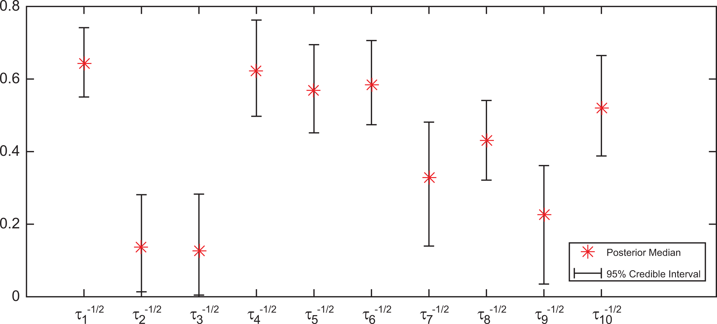
Posterior median and 95% CIs of
6. Conclusion
In this article, we proposed a Bayesian nonparametric two-level hierarchical model for the analysis of one’s latent ability growth in educational testing for longitudinal scenarios. The advantage of our method is able to incorporate the monotonic shape constraints into the estimation of latent trajectories. Due to the flexibility of our nonparametric method, we are able to fit any monotonic continuous curve without further restrictions on the estimation of parameters. Therefore, the estimation of the slopes
The latent trajectories of ability growth estimated from our approach can help educators or practitioners to better understand the behaviors of students in the study, such as the growth patterns (continuous increasing, sharp increasing, and etc.) and the timing that a student reaches the ceiling of increasing for his or her learning ability (i.e., the timing of reaching the plateau). Further studies on clustering those behavioral patterns of individuals will guide us to design education practice or teaching tailored to individuals. In addition, since the evidence of the local dependence assumption is generally strong from the analysis of EdSphere data sets, we can conclude that the use of random effects to model the local dependence seems to be necessary and successful.
As the MCMC computation is time-consuming and resource-demanding for our current approach, our next goal is to improve the efficiency of our computation by developing big data schemes, such as similar ideas of Wei, Wang, and Conlon (2017), to make the parallel computing possible so as to conveniently apply our approach to the entire data sets. With improvement of computation efficiency, we might be able to develop a computable evaluation criterion to assess the model fit of the proposed nonparametric model using the predictive score ideas (Gneiting & Raftery, 2007). Another potential extension is to explore covariates including the grade and others with their relationships to the growth of one’s ability trajectory. This direction will facilitate us to group individuals based on their similar characteristics and encourage the development of personalized education.
Supplemental Material
Supplemental Material, Appendix - Bayesian Nonparametric Monotone Regression of Dynamic Latent Traits in Item Response Theory Models
Supplemental Material, Appendix for Bayesian Nonparametric Monotone Regression of Dynamic Latent Traits in Item Response Theory Models by Yang Liu and Xiaojing Wang in Journal of Educational and Behavioral Statistics
Footnotes
Acknowledgments
The authors are grateful to Dr. Carl Swartz from Highroad Learning company for generously sharing their data with us and to the Editor, Dr. Li Cai, and referees for numerous suggestions that significantly improved this article.
Declaration of Conflicting Interests
The author(s) declared no potential conflicts of interest with respect to the research, authorship, and/or publication of this article.
Funding
The author(s) disclosed receipt of the following financial support for the research, authorship, and/or publication of this article: The research of Dr. Yang Liu was part of his dissertation at the Department of Statistics, University of Connecticut, and was supported by start-up fund from Dr. Xiaojing Wang. Also, Dr. Xiaojing Wang wants to acknowledge the receipt of the National Science Foundation award (#1848451) for support for her research, authorship, and/or publication of this article.
References
Supplementary Material
Please find the following supplemental material available below.
For Open Access articles published under a Creative Commons License, all supplemental material carries the same license as the article it is associated with.
For non-Open Access articles published, all supplemental material carries a non-exclusive license, and permission requests for re-use of supplemental material or any part of supplemental material shall be sent directly to the copyright owner as specified in the copyright notice associated with the article.