
Abstract
This article examines the estimation of two-stage clustered designs for education randomized control trials (RCTs) using the nonparametric Neyman causal inference framework that underlies experiments. The key distinction between the considered causal models is whether potential treatment and control group outcomes are considered to be fixed for the study population (the finite-population model) or randomly selected from a vaguely defined universe (the super-population model). Both approaches allow for heterogeneity of treatment effects. Appropriate estimation methods and asymptotic moments are discussed for each model using simple differences-in-means estimators and those that include baseline covariates. An empirical application using a large-scale education RCT shows that the choice of the finite- or super-population approach can matter. Thus, the choice of framework and sensitivity analyses should be specified and justified in the analysis protocols.
In randomized control trials (RCTs) of education interventions, random assignment is often performed at the group level (such as a school or classroom) rather than at the student level. These group-based designs are common, because education RCTs often test interventions that are targeted to the group (e.g., a school restructuring initiative or professional development services for all teachers in a school). Thus, for these types of interventions, it is infeasible to randomly assign the treatment directly to students.
Under these group-based designs, data are typically collected on students. Thus, using student-level data, the statistical procedures that are used to estimate average treatment effects (ATEs) and their standard errors must account for the potential correlation of the outcomes of students within the same groups. In particular, the standard errors of the ATE estimators must be inflated to account for design effects due to clustering.
Over the past 40 years, a huge statistical literature across multiple disciplines discusses the estimation of treatment effects under two-stage clustered designs (see, e.g., Baltagi & Chang, 1994; De Leeuw & Meijer, 2008; Harville, 1977; Hsiao, 1986; Laird & Ware, 1982; Liang & Zeger, 1986; Murray, 1998; Rao, 1972; Raudenbush & Bryk, 2002; and Wooldridge, 2002). This article contributes to this literature by discussing the estimation of the ATE parameter for clustered designs using the building blocks of the nonparametric model of causal inference that underlies experimental designs. This model was introduced for nonclustered designs by Neyman (1923/1990) and later developed in Rubin (1974, 1977) and Holland (1986) using a potential outcomes framework.
The analysis focuses on continuous outcome data (such as student test scores) that are assumed to be either (1) fixed for the study population (a finite-population [FP] model) or (2) random draws from population outcome distributions (the more common super-population [SP] model). Appropriate estimation methods and new asymptotic variance formulas that are consistent with the Neyman approach are discussed for each model using simple differences-in-means estimators and those that include baseline covariates.
The considered Neyman approach yields estimation equations that have a different error structure than the model-based approaches that are typically used in practice and has several advantages. First, the Neyman approach does not require assumptions on the distributions of potential outcomes (only moment assumptions), whereas the model-based approaches often assume multilevel normality (which may not hold for some educational outcomes such as student absences or teacher salaries). Second, the variance formulas for the FP approach make it explicit that impact findings can be generalized only to those schools and students that are included in the study—which may be realistic in many settings—rather than to a vaguely defined super-population of study units that is often assumed using standard approaches. Finally, unlike commonly used model-based approaches, the Neyman framework allows for heterogeneity of treatment effects, which leads to variance expressions that differ for the treatment and control groups and that differ for the FP and SP models.
An empirical application using a large-scale RCT in the education area shows that the choice of the Neyman FP, the Neyman SP, or the standard model-based approach can matter. These results suggest that education researchers—who currently most often report impact findings using hierarchical linear model (HLM) methods (Raudenbush & Bryk, 2002)—should consider testing the robustness of study findings, by obtaining additional consistent impact estimates using methods that rely on alternative, nonparametric assumptions.
The Neyman Causal Inference Model for Clustered Designs
The FP Model
Consider an experimental design where n groups—hereafter referred to as schools—are randomly assigned to either a single treatment or control condition. The study contains np treatment and n(1 - p) control group schools, where p is the sampling rate to the treatment group (0 < p < 1) (and where np and n(1 - p) are rounded to integers). It is assumed that the study contains mi
students from school i and that there are
It is assumed for now that the n schools and M students define the population universe—the FP model considered by Neyman for nonclustered designs. Under this scenario, the schools and students participating in the study are not considered to have been sampled from some larger population.
Let YTij
be the “potential” outcome for student j in school i in the treatment condition and YCij
be the potential outcome for the student in the control condition. These potential outcomes are assumed to be fixed (true values) for the study. The difference between the two fixed potential outcomes (YTij - YCij ) is the student-level treatment effect, and the ATE parameter β
1 is the ATE over all students:
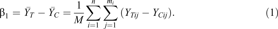
This ATE parameter cannot be calculated directly because potential outcomes for each student cannot be observed in both the treatment and control conditions. Formally, let Ti be the random assignment variable that equals 1 if a school is assigned to the treatment condition and 0 if the school is assigned to the control condition. The data generating process for the observed outcome for a student, yij , can then be expressed as follows:

In Equation 2, yij is a random variable because Ti is a random variable, but the potential outcomes YTij and YCij are fixed for the study. Thus, under the Neyman FP model, the ATE parameter pertains only to those students and schools at the time the study was conducted. Stated differently, the impact findings have internal validity but do not necessarily generalize beyond the study participants. This approach can be justified on the grounds that schools are usually purposively selected for RCTs and, thus, may be a self-selected group of schools that are willing to participate and that are deemed to be suitable for the study based on their populations and contexts. Similarly, students participating in the study may not be representative of all students in the study schools, because they could be a nonrandom subset of those who consented to participate in the study and provided follow-up data.
Under this fixed population scenario, researchers are to be agnostic about whether the study results have external validity. Policymakers and other users of the study results can decide whether the impact evidence is sufficient to adopt the intervention on a broader scale, perhaps by examining the similarity of the observable characteristics of schools and students included in the study to their own contexts, and using results from subgroup impact analyses and analyses measuring the quality and fidelity of intervention implementation across the study sites.
Following the approach for nonclustered designs used by Freedman (2008) and Schochet (2010), a regression model for Equation 2 can be constructed by rewriting Equation 2 as follows:
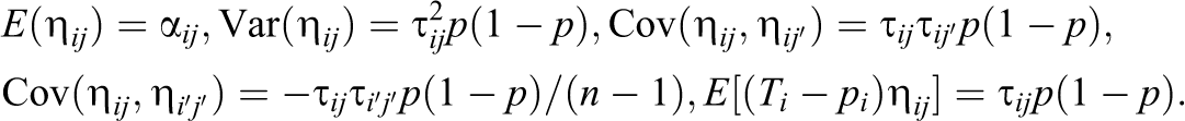
In Equation 3, the error term ηij
is random because it is a function of the random Ti
. The error term is also a function of two nonrandom components: (1)

The model in Equation 3 does not satisfy key assumptions of the usual regression model, because the random error ηij
does not have mean zero (over all possible treatment assignment configurations), and, to the extent that τij
varies across students, ηij
is heteroscedastic,
Equation 3 implicitly assumes that schools are weighted by their student sample sizes. An alternative specification is to weight schools equally. In this case, the ATE parameter is
Importantly, the FP model is very different than a fixed effects model where school effects are treated as fixed and student-level variation within the study schools is assumed to be the only source of variation in the impact estimates. This fixed effects framework does not conform to the Neyman model, because it ignores the randomness in Ti (and thus the clustered nature of the design). Stated differently, both the Neyman FP and fixed effects models assume that the study schools were not sampled, but the FP model treats the assignment of these schools to the treatment and control conditions as random (and adjusts the variance expressions accordingly), whereas the fixed effects approach ignores the randomness of the treatment assignment process and understates the true variance of the impact estimates. Thus, the fixed effects approach is not considered further in this article.
The SP Model
Under the SP version of the Neyman causal inference model, study schools and students are assumed to be random samples from broader populations. Under this framework, students are nested within schools. Let ZTi be the potential outcome for school i in the treatment condition and ZCi be the potential outcome for school i in the control condition. Potential outcomes for the n study schools are assumed to be random draws from potential treatment and control outcome distributions in the study super-population. It is assumed that means and variances of these distributions are finite and denoted by μT and σuT 2 for potential treatment outcomes and μC and σuC 2 for potential control outcomes.
Suppose next that mi
students are sampled from the super-population of students in study school i. The potential student-level outcomes YTij
and YCij
are now assumed to be random draws from student-level potential outcome distributions (which are conditional on school-level potential outcomes) with respective means ZTi
and ZCi
and finite variances
Under the SP model, the ATE parameter is
In the SP framework, Ti , ZTi , ZCi , YTij , and YCij are all random variables. As before, we can use Equation 2 to express observed student outcomes in terms of potential outcomes and can rearrange terms to yield the following regression model:
Furthermore, if we define


Thus, this model is the usual random effects model with an exchangeable mi xmi
positive definite variance–covariance matrix for subjects within each school (labeled as
Finally, note that Equation 4 can also be derived using the following two-level HLM model (Bryk & Raudenbush, 1992):

ATE Parameter Estimation for the FP Model
This section discusses ATE parameter and variance estimation for the FP model with and without baseline covariates. Proofs of asymptotic results are provided in online supplement Appendix A. We rely on asymptotic results because the regression estimators are complex functions of the random variable Ti , which makes it difficult to obtain finite-sample moments. To obtain asymptotic properties for the estimators, we consider an increasing sequence of finite populations with the number of schools n increasing to infinity.
The FP Model Without Covariates
Ordinary least squares (OLS) methods are appropriate for estimating β
1 in Equation 3, because the ATE parameter for the FP model pertains to the study sample only. The following lemma provides the asymptotic moments of the OLS estimator.
Lemma 1. The simple OLS estimator for β
1 under the FP model in Equation 3 is
where
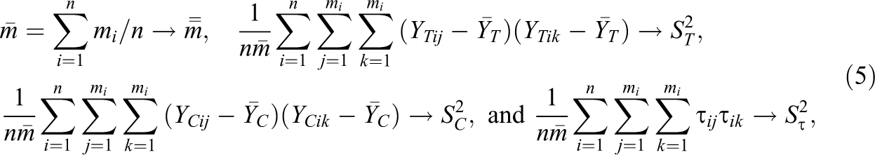

The ST 2 and SC 2 terms pertain to the extent to which potential outcomes vary and covary across students within the same schools. The S_τ 2 term pertains to the extent to which treatment effects vary and covary across students within schools. Note that if student-level treatment effects are constant, S_τ 2 = 0 and ST 2 = SC 2.
Consistent estimators for ST 2 and SC 2 in Equation 6 can be obtained using sample variances and covariances for treatments and controls, sT 2 and sC 2, respectively:

where
Consistent estimators for S_τ
2 in Equation 6 take the form
Subgroup method
Under this approach, ATEs can be estimated for a large number of student- and school-level subgroups defined at baseline by regressing yij on treatment-by-subgroup interaction terms. Estimates for τi can then be obtained using predicted ATEs from these subgroup interaction models. This approach may underestimate s_τ 2 because the estimates for τij are constant within subgroup cells, and the subgroup covariates may not fully explain the variation in τij . However, this approach is fully based on the experimental design.
Propensity score matching method
This method uses propensity score matching (Rosenbaum & Rubin, 1983) to match treatment and control subjects using baseline data. This can be done in two stages by first matching treatment and control schools and then matching subjects within those schools, or in one stage by directly matching treatment and control subjects where school-level variables are included as matching covariates. Nearest neighbor, caliper, kernel, or similar matching methods with replacement could be used for the analysis (see Smith & Todd, 2005).
Note that there may be instances where covariates are not available to estimate S_τ
2. In this case, because

which is a conservative FP variance estimator.
Finally, if schools are to be weighted equally under unbalanced designs, the estimators from above can be applied by first premultiplying the outcome and explanatory variables (including the intercept) by the weights
The FP Model With Covariates
We now examine ATE estimators when the FP models include a 1xv vector of fixed covariates,
Importantly, in the Neyman model with fixed covariates, Equation 3 is still the true model. Thus, the ATE parameters considered above in the models without covariates pertain also to the models with covariates. To the extent that the covariates have explanatory power, they will be correlated with the error terms in Equation 3 (which violates a key assumption of the usual regression model).
To examine asymptotic moments of the OLS estimator under the FP model with fixed covariates, we assume in addition to Equation 5 that as n approaches infinity:
Lemma 2. Let


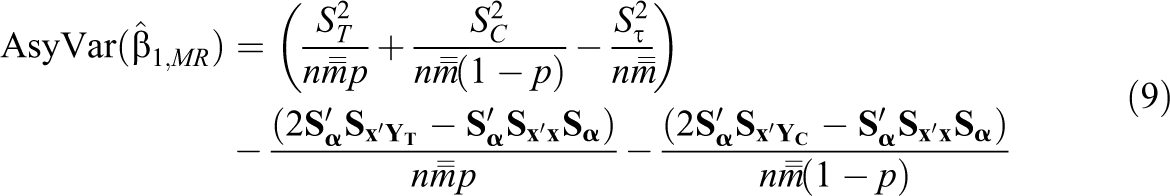
The first bracketed term in Equation 9 is the variance of the OLS estimator under the FP model without covariates. The remaining terms account for precisions gains (or losses) from covariate adjustment.
Consistent estimators for the
ATE Parameter Estimation for the SP Model
This section examines ATE parameter estimation for the SP model with and without baseline covariates using generalized least squares (GLS) methods that are often used to estimate random effects models. It is assumed that the cluster sample sizes mi
are randomly distributed across schools and thus are uncorrelated with Ti
,
The SP Model Without Covariates
Let
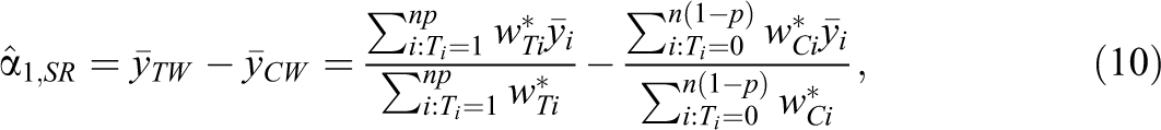
where
The GLS estimator in Equation 10 is a weighted differences-in-means estimator, where the weights are inverses of the variances of school-level means. Schools with more sampled students receive more weight than smaller schools, because the larger schools provide more information on the super-population parameters μT
and μC
. The SP weights will lie between the subject-level FP weights where schools are weighted by their sample sizes and the school-level FP weights, where schools are weighted equally. The SP weights will converge to the subject-level weights as the intraclass correlations (ICCs),
Assume that as n approaches infinity,
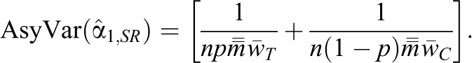
The terms in Equation 11 are comparable to the ST 2 and SC 2 terms in Equation 6 for the FP model. Thus, an important difference between the SP and FP models is that unlike the SP model, the FP model contains S_τ 2, which reduces variance. Thus, the variance may be somewhat smaller under the FP model, which is expected, because the SP model assumes external validity, with an associated loss in statistical precision.
The asymptotic variance in Equation 11 can be estimated as follows:
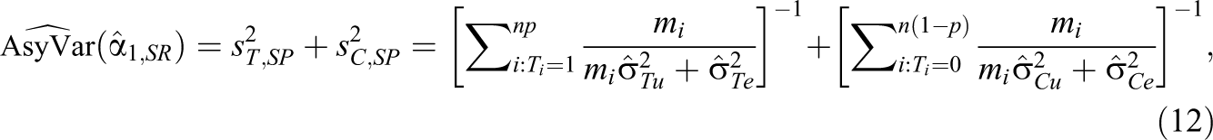
where estimated values for the variance components can be obtained using standard full or restricted information maximum likelihood (FIML or REML) methods (that assume normality of the errors), ANOVA, MINQUE, or similar approaches (see, e.g., Baltagi & Chang, 1994, and De Leeuw & Meijer, 2008).
The SP Model With Covariates
Under the SP model with covariates, the covariates xijl
and potential outcomes are considered to be random draws from joint school- and student-level super-population distributions. Let
The SP model can include “school-level” covariates (e.g., indicators of the school’s urban or rural status) that are modeled as
In the SP model with covariates, Equation 4 remains the true model. Similarly,
To examine asymptotic moments of the GLS estimator under the SP model with covariates, we assume the following population moment analogs to Equation 8 for the FP model:
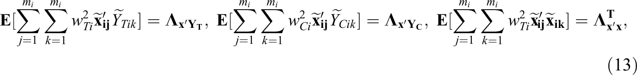
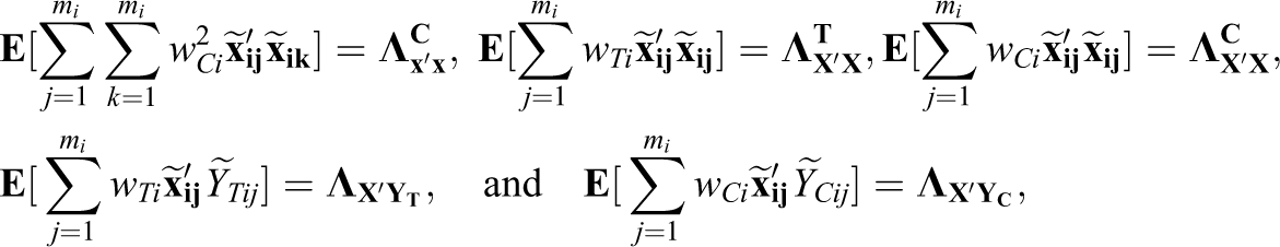
where
The (finite) elements of the
The following lemma provides the asymptotic distribution of the GLS SP regression estimator (Yang & Tsiatis, 2001, and Schochet, 2010, provide OLS results for nonclustered SP designs). The proof is provided in Appendix A.
Lemma 3. Let
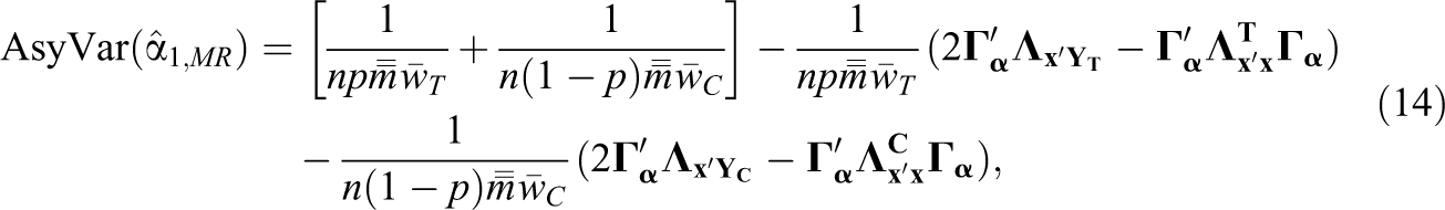
The form of Equation 14 is similar to the form of Equation 8 for the FP model and has a similar interpretation. The first bracketed term is the variance of the GLS estimator under the SP model without covariates. The remaining terms account for precision effects due to covariate adjustment.
The
Empirical Application
The section compares impact findings using the FP and SP estimators discussed above using data from a large-scale school-based RCT of the achievement effects of four early elementary school math curricula (Agodini, Harris, Atkins-Burnett, Heavside, & Novak, 2009) that was funded by the Institute of Education Sciences (IES) at the U.S. Department of Education (ED). Table 1 describes the evaluation design, data, samples, key outcome measures, and baseline covariates. The impact results presented in the evaluation report were obtained using the standard random effects REML estimator, which assumes the same error structure for treatments and controls and that the errors are conditional on the covariates.
Summary of Data Source Used for the Empirical Analysis

Note: IES = Institute of Education Sciences.
a. Variables were used to estimate potential outcomes using the subgroup method described in the text but not as baseline covariates.
For this article, the data were reanalyzed using the various FP and SP estimators considered above with and without covariates. Standard errors for the FP models were obtained using Equations 6 and 9, where sample moments were used to estimate ST
, SC
, and the
Standard errors for the SP model were obtained using Equations 11 and 14. The Swamy and Arora (SA, 1972) ANOVA method was used to estimate the variance components σu.
2 and σe.
2 in Equation 4 that were needed to calculate the weights wTi
and wCi
. The SA ANOVA method, which is based on residuals from within- and between-school OLS regressions, was used rather than REML or FIML methods, because the SA ANOVA method does not rely on distributional assumptions (and thus, is more in line with the nonparametric Neyman framework), and was shown by Baltagi and Chang (1994) to perform well in simulations. Elements of the
Before presenting the impact findings, it is important to first present several key features of the data that can be used to help interpret the impact estimates. First, sample sizes vary across the study schools (the range is 16–51 students and the median is 31 students per school), and the ICC for the SP model without covariates is about 0.19 for both treatments and controls. Thus, the way in which school-level means are weighted to produce overall impacts will differ for the FP and SP models, which could lead to different impact findings across the estimators.
Second, the error structure is similar for treatments and controls. For example,
Finally, the value of
Table 2 displays impact findings for the considered FP and SP estimators, the standard REML estimator, and the GEE empirical sandwich estimator. All estimators yield similar overall impact findings. The models with covariates all show that the Saxon or Math Expressions math curriculum produced significantly higher fifth-grade student math test scores than the other tested math curricula. The estimated impacts are all about 2.30 scale points, which translates into an impact of about 0.27 standard deviation (effect size) units, or about 3 months of average learning growth in math per year for these students (see Schochet, 2008). The impact estimates for the models without covariates are not statistically significant for any estimator due to the omission of the pretests that considerably improve the precision of the impact estimates.
Impact Findings, by Estimator
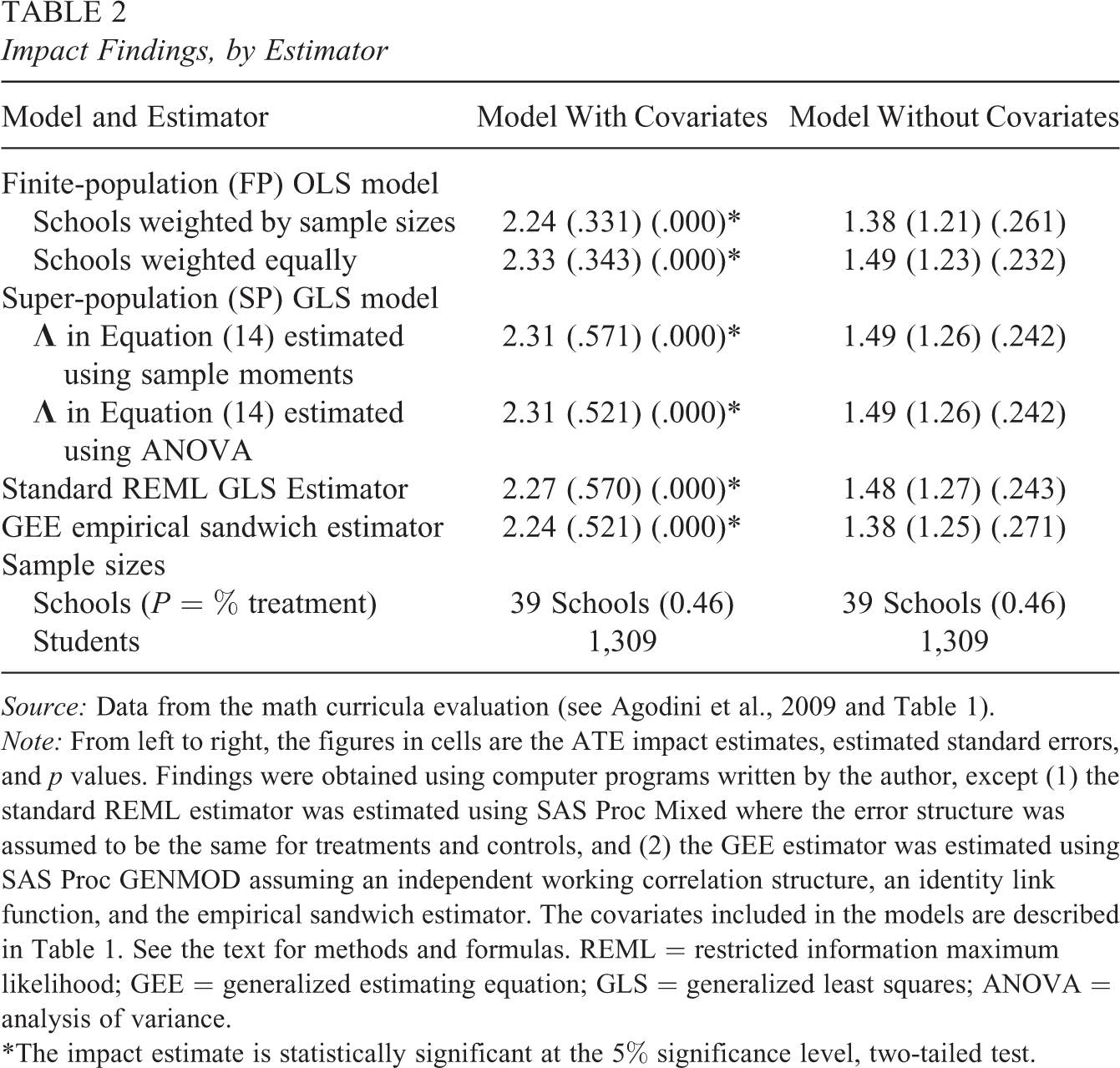
Source: Data from the math curricula evaluation (see Agodini et al., 2009 and Table 1).
Note: From left to right, the figures in cells are the ATE impact estimates, estimated standard errors, and p values. Findings were obtained using computer programs written by the author, except (1) the standard REML estimator was estimated using SAS Proc Mixed where the error structure was assumed to be the same for treatments and controls, and (2) the GEE estimator was estimated using SAS Proc GENMOD assuming an independent working correlation structure, an identity link function, and the empirical sandwich estimator. The covariates included in the models are described in Table 1. See the text for methods and formulas. REML = restricted information maximum likelihood; GEE = generalized estimating equation; GLS = generalized least squares; ANOVA = analysis of variance.
*The impact estimate is statistically significant at the 5% significance level, two-tailed test.
Importantly, however, the estimated standard errors for the models with covariates are about 40% smaller using the FP estimators than the SP estimators. As discussed, this primarily occurs because, unlike the SP estimators, the variances of the FP estimators are reduced by
Summary and Conclusion
This article has examined the estimation of two-stage clustered RCT designs in the education area using the Neyman causal inference framework that underlies experiments. The key distinction between the considered causal models is whether potential treatment and control group outcomes are considered to be fixed for the study population (the FP model) or randomly selected from a vaguely defined super-population (the SP model).
In the FP model, the only source of randomness is treatment status, and a clustered design results only because students in the same cluster share the same treatment status. The relevant impact parameter for this model is the ATE for those in the study sample; thus, the impact results are internally valid only. In the SP model, cluster- and student-level potential outcomes are considered to be randomly sampled from respective super-population distributions. In this framework, the relevant ATE parameter is the intervention effect for the average cluster in the super-population. Thus, impact findings are assumed to generalize outside the study sample, although it is often difficult to precisely define the study universe.
This article derived asymptotic variance formulas for models with and without baseline covariates using OLS methods for the FP model and GLS methods for the SP model. The key difference between the FP and SP variance formulas is that the FP variance is reduced by a S_τ term that pertains to the extent to which treatment effects vary and covary across students within schools. Another important difference between the FP and SP variance estimators is the way in which schools are weighted for the analysis.
Importantly, the considered estimators differ from the standard model-based HLM estimator that is typically used in practice for clustered education RCTs, mainly due to differences in the assumed model error structures. This largely occurs because the Neyman framework allows for heterogeneity of treatment effects, which leads to variance expressions that differ for the treatment and control groups (which the HLM approach can accommodate but which is often ignored in practice). In addition, the HLM model is an SP approach, and thus, cannot accommodate the FP approach, and in particular, the reduction in variance due to treatment effect heterogeneity under the FP model. Furthermore, the Neyman approach does not require assumptions on the distributions of potential outcomes, whereas the model-based approaches typically assume multilevel normality, which may not always hold. Finally, in models with covariates, the variance–covariance matrix of the error terms in the HLM model is assumed to be conditional on the covariates, whereas the covariates do not enter the true model under the Neyman approach; this leads to differences in how clusters (schools) are weighted in the analysis to obtain overall impact estimates.
Using data from a recent influential clustered RCT in the education area, the empirical analysis estimated ATEs and their standard errors using the FP, SP, and standard HLM and GEE estimators. All estimators yield similar ATE point estimates and findings concerning statistical significance. However, standard errors of the FP estimators are considerably smaller than for the other estimators due to the S_τ term. This suggests that in particular studies, policy conclusions could differ using the various approaches.
As shown in this article, the decision to adopt the FP or SP framework in clustered RCTs can matter and has implications for the way in which the impact findings are generalized and interpreted. The choice of the benchmark estimation method should best fit evaluation research questions and objectives and should be specified and justified in the analysis protocols. The choice of framework, however, is often a difficult philosophical issue, and there might not always be a scientific basis to help guide this decision. Thus, education researchers may want to consider specifying in their analysis protocols sensitivity analyses using alternative estimation approaches and attempt to explain any discrepancies between sensitivity and benchmark analysis findings.
Footnotes
Declaration of Conflicting Interests
The author declared no potential conflicts of interest with respect to the research, authorship, and/or publication of this article.
Funding
The author disclosed receipt of the following financial support for the research and/or authorship of this article: This research was funded under Contract ED-04-CO-0112/0006 with the U.S. Department of Education.
References
Supplementary Material
Please find the following supplemental material available below.
For Open Access articles published under a Creative Commons License, all supplemental material carries the same license as the article it is associated with.
For non-Open Access articles published, all supplemental material carries a non-exclusive license, and permission requests for re-use of supplemental material or any part of supplemental material shall be sent directly to the copyright owner as specified in the copyright notice associated with the article.