A Semiparametric Model for Jointly Analyzing Response Times and Accuracy in Computerized Testing

Abstract

The item response times (RTs) collected from computerized testing represent an underutilized type of information about items and examinees. In addition to knowing the examinees’ responses to each item, we can investigate the amount of time examinees spend on each item. Current models for RTs mainly focus on parametric models, which have the advantage of conciseness, but may suffer from reduced flexibility to fit real data. We propose a semiparametric approach, specifically, the Cox proportional hazards model with a latent speed covariate to model the RTs, embedded within the hierarchical framework proposed by van der Linden to model the RTs and response accuracy simultaneously. This semiparametric approach combines the flexibility of nonparametric modeling and the brevity and interpretability of the parametric modeling. A Markov chain Monte Carlo method for parameter estimation is given and may be used with sparse data obtained by computerized adaptive testing. Both simulation studies and real data analysis are carried out to demonstrate the applicability of the new model.

Keywords

response time Cox proportional hazards model partial likelihood Markov chain Monte Carlo

1. Introduction

Response times (RTs) on test items provide a valuable source of information on examinees and test items. For instance, RTs can help in evaluating the speededness of the test, offering collateral information for calibrating test items and estimating examinees’ abilities, and they can be used for detecting cheating behaviors and designing a better test (e.g., Bridgeman & Cline, 2004; Fan, Wang, Chang, & Douglas, 2012; van der Linden & Guo, 2008). With the prevalence of computerized testing, their collection has become straightforward. To make full use of RTs to enhance online testing’s efficiency and security, appropriate psychometric models for RTs should be developed.

In the past decades, researchers have been trying to formulate models that can maximally explain the variance of RTs as well as the connections among RTs, item characteristics, and examinees’ behaviors. Most of the models are motivated by the curve-fitting principle in the sense that the proposed models are parametric representations of the underlying RT distributions (e.g., Klein Entink, van der Linden, & Fox, 2009; Rounder, Sun, Speckman, Lu, & Zhou, 2003; Schnipke & Scrams, 1997). Although parametric models have the advantage of conciseness, they may suffer from reduced flexibility to fit real data. In addition, with an unknown data set, one often needs to fit each parametric model separately until a best fitting model is decided based upon some model diagnostic criterion (Schnipke & Scrams, 1997). However, the best fitting model may not be the best one for each individual item in the item bank. A recent example presented in Ranger and Kuhn (2011) demonstrated that item RT distributions differed dramatically from one test to another, which calls for the need of a flexible model that relaxes such distributional assumptions.

To simplify the fitting procedure and to emphasize the individual characteristics of each item, Ying and Chang (2005) suggested constructing a “generalized model” that subsumes various parametric models as submodels. By fitting the generalized model to a data set, one can immediately pinpoint the most appropriate parametric form for each item from the estimation results. One such example is the Box-Cox normal model (Klein Entink et al., 2009), in which a power parameter is introduced to represent a number of different transformations. Most recently, Ranger and Kuhn (2011) proposed a generalized linear model with a flexible link function to model discrete RTs. Specifically, their model includes a shape parameter (either item level or test level) that determines the form of the link function, and their model unifies both proportional hazards (PH) models and accelerated lognormal failure time models. A common ground for the above two general models is they both contain an item-level parameter that controls the shapes of the RT distributions, and they are still parametric models. In this article, we propose a semiparametric approach that combines the flexibility of nonparametric modeling and the brevity of the parametric modeling. To be specific, we propose a hierarchical PH frailty model. We will show how the new models exhibit greater flexibility than the previous proposed parametric models. A two-stage estimation method is developed for model calibration, and methods for model diagnosis are presented.

1.1. Survival Analysis and RT Modeling

Survival analysis is a branch of statistics which concerns the analysis of time-to-event data. Survival analysis has benefited medical scientists in the study of mortality due to chronic diseases and has helped industrial statisticians to model the longevity of machinery and parts in manufacturing processes. In principle, survival analysis techniques could be used in any science in which outcomes are measured as the time until an awaited event. Psychology is also a specific area that survival analysis can shed light on. For instance, Douglas, Kosorok, and Chewning (1999) proposed a discrete version of the PH frailty model to explain substance abuse of youths. In particular, they modeled the ages at which youths first tried alcohol, cigarettes, marijuana, and inhalants, as a function of their latent psychological abilities to abstain from substance abuse. Another example is by Singer and Willett (1993), who used discrete-time survival analysis to study when public school teachers stopped teaching between their year of hire and the year when the data collection ended. The discrete-time hazard model proposed in their paper not only answers these descriptive questions but also models the relationship between event occurrence and predictors. One specific area in educational measurement that survival analysis comes into play is RT analysis. RT is the time period from the onset of an item until the examinee provides an answer to the item. If viewing “giving a response” as an event, RT shares the same meaning as the survival time in biostatistics, and therefore RTs can be modeled similarly.

Many regression models have been proposed in survival analysis to account for the effect of the explanatory covariates. Oftentimes, the covariates enter into the model through the hazard function. The hazard function (usually denoted as $h (t)$ ) is the instantaneous rate at which events occur. It is defined as

h (t) = lim_{δ t \to 0} \frac{P [t \leq T < t + δ t | T \geq t]}{δ t} .

In psychological terms, the hazard rate is the conditional probability of finishing the task in the next moment; thus, it is viewed as the processing capacity of an individual. In other words, the hazard rate measures the individual’s relative ability to perform mental work in a unit of time. High hazard rates correspond to a high processing capacity and indicate that the examinee works more intensely (Wenger & Gibson, 2004). The hazard rate relates to the survival function through $S (t) = exp [- H (t)],$ where $H (t) = \int_{s = 0}^{t} h (s) d s$ is the cumulative hazard function. One common regression model takes the form

h (t | Z = z) = h_{0} (t) c (z^{'} β),

where $h_{0} (t)$ is the baseline hazard rate that does not depend on the covariates. The covariate Z can be any observed variable, and in Model 1, the effects of the covariates are reflected through a linear form $Z^{'} β$ . $β^{'} = (β_{1}, . . ., β_{p})$ are regression parameters and c is a specified functional form. The choice of c depends on the particular data being considered, and three common forms have been used in the past: (1) $c (Z) = 1 + Z$ , (2) $c (Z) = (1 + Z)^{- 1}$ , and (3) $c (Z) = exp (Z)$ . The first two forms correspond to (1) the hazard rate and (2) mean survival time, being linear functions of $Z$ . The last form, which is also the most widely used form, assumes that a unit increase in a covariate is multiplicative with respect to the hazard rate. Because of this, Model 1 with $c (\cdot)$ taking the last form is called relative risk model or proportional hazards model.

When $h_{0} (t)$ takes on parametric forms, Model 1 becomes a parametric model. When $h_{0} (t)$ is nonparametrically defined, then Model 1 becomes a semiparametric model, also named as the Cox PH model (Cox, 1972). Here the nonparametric baseline hazard $h_{0} (t)$ reflects the flexibility of the model to accommodate a variety of different shapes of RT distributions, whereas the regression term succinctly summarizes how RTs change with the covariates. When the baseline hazard is a constant, this model becomes the exponential regression model; when the baseline hazard takes the form of $h_{0} (t) = γ (λ t)^{γ - 1}$ , the model becomes the Weibull regression model. In light of this, the Cox model is flexible enough to represent different RT distributions, and thus it serves as a good candidate for modeling RTs.

In the above models, the covariates are assumed to be observed. Biostatisticians first recognize the usefulness of latent variables to model survival times that are correlated due to either repeated measurements taken on a single subject, or measurements of a common variable taken on genetically associated subjects. These needs give rise to frailty models, in which a latent frailty random variable is included in the model to account for possible correlations in failure time distributions (Clayton, 1991; Clayton & Cuzick, 1985). The frailty variables may be viewed as random effects and usually only the influence of the explanatory covariates on failure time is the primary concern. Douglas et al. (1999) used the frailty model in psychology, and their model is a similar version of the conditional PH model (Clayton & Cuzick, 1985), in which the hazard function for each failure time is a product of the baseline hazard, frailty random variable, and covariate effects. The unique feature of their model is that it has an item-level parameter that measures the influence of the latent variable on the failure time. Thus separate items differ with respect to the extent that the latent variable influences responses. In fact, the Cox PH model represents a standard approach in survival time analysis, it makes only very mild distributional assumptions and is a flexible semiparametric model. However, it is only very recently that the Cox model has been introduced in the field of measurement to analyze RTs (Ranger & Ortner, 2011). This article is complementary to the existing parametric approaches and Ranger and Ortner’s earlier research.

1.2. RT Modeling

RT has been a preferred dependent variable in cognitive psychology since the mid-1950s (Luce, 1986). For relatively uncomplicated cognitive tasks such as Posner’s perceptual matching task (Posner & Boies, 1972), RTs naturally indicate the processing procedures of each individual. In educational testing, RTs are usually analyzed along with the response accuracy. Such models include Thissen (1983), van der Linden (2007), Roskam (1997), Wang and Hanson (2005), among others. Most of these models are motivated by the idea of a speed-accuracy relationship. Cognitive psychologist often focus on the within-person relationship, that is, whether a person’s response accuracy will decrease if he or she chooses to perform a task more quickly? This is termed as speed–accuracy trade-off. Psychometricians, however, are more interested in the across-person relationship between speed and accuracy. For example, one question that psychometricians often explore is whether examinees with higher ability tend to answer items faster. Both types of speed–accuracy relationships are considered within the model suggested by Verhelst, Verstralen, and Jansen (1997). In their models, the speed–accuracy trade-off is reflected by letting response accuracy depend on the time devoted to the item—spending more time on an item increases the probability of a correct response. The speed–accuracy correlation across examinees is reflected by the separate parameters of examinees’ ability (or mental power) and speed.

Van der Linden (2007) argued that although the speed–accuracy trade-off is prevalent in reaction-time research, on a test with a reasonable time limit, there is no need to incorporate a trade-off in an RT model for a fixed person and a fixed set of test items. In other words, the trade-off is a within-person constraint only. Thus, the speed at which the test taker operates on the items should be assumed as a latent trait, and the response accuracy should only be determined by the examinees’ abilities. This conclusion is supported by Tate (1948), who investigated the speed accuracy relationship on number series, arithmetic reasoning, and spatial relations questions. He found that when accuracy is controlled, the fastest examinees are not the most accurate but fast subjects are consistently fast and slow subjects are consistently slow. These research results indicate that we need to model accuracy exclusively dependent on ability, and RT exclusively dependent on examinees’ latent speeds. But on the higher level, the speed and ability variables may be correlated. The correlation may differ depending upon the test context and content (Schnipke & Scrams, 2002). Following this argument, van der Linden (2007) proposed a hierarchical framework, in which RT and responses are modeled separately at the measurement model level; and at a higher level, a population model for the person parameters (speed and ability) is constructed to account for the correlation between them. This framework allows “plug-and-play” in that one can insert different measurement models in the first level and assume different covariance structures in the second level. The new model we will present in the next section is one application of this framework.

2. Semiparametric RT Model

We propose a hierarchical PH model to model RTs and response accuracy simultaneously. A critical feature of the models is that we distinguish examinees’ abilities from their latent speed and assign separate latent traits to both of them. This leads to the key assumption of the current model: A test taker operates at a fixed level of speed during the course of the tests. This stationarity assumption excludes changes in behavior during the test due to fatigue, learning, strategy shifts, and other factors. The hierarchical framework proposed by van der Linden (2007) is adopted here. Measurement models at the first level separate the variability in the observed responses and RTs into item and person effects. At a higher level, we assume the examinee’s ability θ and latent speed τ are from a bivariate normal distribution. The specific formulation of the model is as follows.

2.1 First-level model. At the first level, two models for the responses and RTs are specified separately. For the item response model, any appropriate parametric model may be used, but we focus on the three-parameter logistic model:

P_{j} (θ_{i}) = c_{j} + (1 - c_{j}) \frac{exp [a_{j} (θ_{i} - b_{j})]}{1 + exp [a_{j} (θ_{i} - b_{j})]},

with $a_{j}$ , $b_{j}$ , and $c_{j}$ representing item discrimination, difficulty, and guessing parameters. For the RTs, the Cox PH model is chosen and the hazard function for RTs is

h_{i j} (t | τ_{i}) = h_{0 j} (t) exp (β_{j} τ_{i}),

with the survival function being

P (t_{i j} \geq t | τ_{i}) = S_{i j} (t) = exp [- \int_{0}^{t} h_{0 j} (s) exp (β_{j} τ_{i}) d s],

where $τ_{i} \in R$ is the speed parameter for test taker i. The subscript j in $h_{0 j}$ implies that different shapes of the RT distributions are possible for different items, and $β_{j}$ is the regression parameter (i.e., slope). Parameter $β_{j}$ is constrained to be positive, implying that higher $τ_{i}$ yields shorter RTs. In this regard, $β_{j}$ can also be viewed as a discrimination parameter. Notice that constraining $β_{j}$ to be positive also removes the possible sign reversion between $τ_{i}$ and $β_{j}$ , such that the model is identifiable. This measurement model resembles the one proposed by Ranger and Ortner (2011). The $β_{j}$ coefficient also determines the influence of the latent speed on the hazard rate. In a psychological sense, it controls the increase in processing capacity that is due to a unit increase in the latent speed. Notice that in traditional survival analysis, the regression parameter is interpreted in a relative sense. But in educational measurement, it is important to be able to make inference about examinees and items, such as how much time is required for each examinee on a particular item on average. Therefore, both the regression parameter and the baseline hazard have to be estimated accurately. This point is reemphasized in the model estimation section below. As every constant multiplier can be absorbed in the baseline hazard rate, the linear predictor $β_{j}$ $τ_{i}$ does not include an intercept term. The item time intensity is reflected in the baseline hazard, and more clearly via Equation 4. In general, items with lower cumulative hazard $H_{0} (t)$ tend to be more time consuming.

2.2 Second-level model. This part of the model captures the joint distribution of the person parameters in a population. The values of $ξ_{i} = (θ_{i}, τ_{i})^{'}$ are assumed to be randomly drawn from a bivariate normal distribution, that is,

ξ_{i} ~ f (ξ_{i}; μ_{p}, \sum_{p}) \equiv \frac{| \sum_{p}^{- 1} |^{1 [2}}{2 π} exp [- \frac{1}{2} (ξ_{i} - μ_{p})^{^{'}} \sum_{p}^{- 1} (ξ_{i} - μ_{p})],

with mean vector

μ_{p} = (μ_{θ}, μ_{τ}),

and covariance matrix

\sum_{p} = (\begin{matrix} σ_{θ}^{2} & σ_{θ τ} \\ σ_{θ τ} & σ_{τ}^{2} \end{matrix}) .

2.3 Identifiability. To establish identifiability, we suggest the constraints $μ_{θ} = 0, σ_{θ}^{2} = 1, μ_{τ} = 0, σ_{τ}^{2} = 1$ . Here, the first two constraints are standard in IRT parameter estimation, when item parameters are unknown. The last two constraints fix the scale of τ to remove the trade-off between $β_{j}$ and $τ_{i}$ and they also fix the scale of h ₀.

In van der Linden’s (2007) model, he imposed a covariance structure on item parameters, whereas we assume that item parameters are independent of one another. There are three reasons. First, according to the results in van der Linden (2007), only the correlation between item time intensity and item difficulty is nonzero (with posterior mean 0.3), all the rest correlations are either very close to 0 or have posterior confidence interval covering 0. Second, the item time intensity information in the new model is reflected in the nonparametric baseline hazard $h_{0 j} (t)$ , whose correlation with the item difficulty $b_{j}$ is not easily modeled. Only when the parametric form of $h_{0 j} (t)$ is known, for instance, in exponential model, $h_{0 j} (t) = λ_{j}$ , that one can model the correlation between λ and b. In this case, because $S_{i j} (t) = exp [- exp (β_{j} τ_{i}) (λ_{j} t)]$ , λ and b should be negatively correlated, indicating that more difficult items are more likely to be time consuming. Third, as shown in our simulation study below, even when the correlation between item time intensity and item difficulty is ignored, the estimation accuracy will not be significantly affected.

3. Model Estimation

The goal of our investigation is to accurately estimate θ and τ, as well as the regression parameter β in RT model of Eqaution 4 and item parameters in Equation 2. In many Cox frailty model applications, only the regression parameter β and frailty τ need to be estimated, but in our case, in order to make inference about the examinees and items, the nonparametric cumulative baseline hazard H ₀ also needs to be estimated. Several approaches are proposed in the past to estimate both parametric and nonparametric parts of the Cox model, such as estimation based on a spline approximation of the baseline hazard rate (Cai, Hyndman, & Wand, 2002) or estimation based on piecewise exponential models (Friedman, 1982). Two approaches that have advantages (Ranger & Ortner, 2011) are (1) estimation by treating RT as a discrete variable (McCullagh, 1980), such that the Cox model can be viewed within the generalized linear model framework and standard software can be used for model estimation; (2) estimation based on profile likelihood; this approach does not require categorization of the RTs and thus it is more efficient (Ranger & Ortner, 2011). In this study, we propose a two-stage estimation method that employs a divide-and-conquer strategy, specifically, we estimate the parametric part first and nonparametric part second. Instead of using the marginalized maximum likelihood framework as in Ranger and Ortner (2011), we use the Markov chain Monte Carlo (MCMC) framework which is more flexible.

Marginal likelihood inference involving latent variables is usually challenging because of the integrals that are sometimes numerically intractable. One approach that avoids such difficulties is to use the MCMC method to obtain draws from a distribution that has a density proportional to the joint posterior distribution of the item and person parameters. Another motivation for using the MCMC method is that in computerized adaptive testing (CAT), every test taker is given different items, based on his or her adaptively estimated θ level. So the random sampling of θ (or τ due to the possible correlation between them) from a common distribution can not be assumed. We wish for our estimation technique to allow for data obtained by CAT. Consequently, the usual marginal likelihood approaches used in latent variable modeling are no longer appropriate.

Estimating Cox’s PH frailty model with MCMC is not entirely new. Clayton (1991) used Gibbs sampling to fit frailty models to clustered failure data. He sampled iteratively from the full conditional distribution of $H_{0 j}$ and all parameters with $H_{0 j}$ as an independent increment gamma process (Kalbfleisch, 1978). Gray (1994) used a piecewise constant baseline hazard and also included it as a parameter to be updated in the MCMC scheme. Similarly, Douglas et al. (1999) modeled the discrete failure time, and treated the baseline hazard as a constant at each time point, which again was incorporated in the MCMC algorithm. Most recently, Henschel, Engel, Holzel, and Mansmann (2009) treated the baseline hazard with a stepwise constant function as well as a cubic spline. Sharef, Strawderman, Ruppert, Cowen, and Halasyamani (2010) argued that treating baseline hazard as piecewise constant is somewhat too restrictive because it depends on some discretization of time. Instead, they proposed to model the baseline hazard as a penalized mixture of B-splines. Their approach is even more general in that they allowed the frailty distribution to be unspecified, and modeled it as a penalized mixture of normalized B-splines. As a result, their model estimation method continues to apply to the PH frailty model, while it permits shrinkage toward a specific parametric hazard function or frailty distribution.

Although the Sharef et al. (2010)’s method is flexible and promising, it does not lend itself directly to our case because of two reasons: (1) In our model, we assign an item level regression coefficient $β_{j}$ in front of the frailty term $τ_{i}$ , whereas in their model, the effect of the frailty is the same across different items; (2) in our model, we impose a covariance structure on the frailty term, which introduces extra difficulty in model estimation. Due to these reasons, we propose a two-stage estimation method. In the first stage, we avoid the difficulty of modeling and sampling from $H_{0 j}$ using the Cox partial likelihood (Cox, 1972), and in the second stage, we estimate the infinite-dimensional parameter $H_{0 j}$ either through nonparametric estimator or through B-splines. The use of partial likelihood in the Bayesian context for the frailty model estimation has been demonstrated in Gustafson (1997) and Sargent (1998). The justification for using partial likelihood will be briefly described in section 3.2.2.

3.1. Partial Likelihood

For the jth item, suppose that there are no ties between the RTs. Let $t_{(1 j)} < t_{(2 j)} < \dots < t_{(N j)}$ denote the ordered RTs and $τ_{i}$ be the latent trait associated with the individual whose RT is $t_{(i j)}$ . Define the risk set $R (t_{(q j)})$ at time $t_{(q j)}, 1 \leq q \leq N$ , as the set of all individuals who have not answered the question yet, that is, $R (t_{(q j)}) = {t_{((q + 1) j)}, \dots, t_{(N j)}}$ . The partial likelihood function for the jth item given τ is specified as:

\begin{aligned} L (β_{j} | τ) = \prod_{i = 1}^{N} \frac{exp [β_{j} τ_{i}]}{\sum_{t_{q j} \in R (t_{(i j)})} exp [β_{j} τ_{q}]} \\ = \prod_{i = 1}^{N} \frac{exp [β_{j} τ_{i}]}{\sum_{q \geq i}^{N} exp [β_{j} τ_{q}]} . \end{aligned}

The partial likelihood for the vector $β = (β_{1}, \dots, β_{J})^{'}$ is then defined as

L (β | τ) = \prod_{j = 1}^{J} L (β_{j} | τ) .

Kalbfleisch and Prentice (1973) demonstrated that the partial likelihood is a marginal likelihood for β arising out of the distribution of the rank vector associated with the failure times (or RTs). The use of the partial likelihood for inference on β has been justified from both the frequentist viewpoint (Anderson, Borgan Gill, & Keiding, 1982) and the Bayesian viewpoint (Kalbfleisch, 1978).

3.2. Parameter Estimation: MCMC

For the ith test taker, his or her responses and RTs are denoted by $Y_{i} = (Y_{i 1}, \dots, Y_{i J})^{'}$ , and $T_{i} = (T_{i 1}, \dots, T_{i J})^{'}$ , respectively. We model the jth item’s hazard function by Equation 3 and specify the partial likelihood function by Equation 6. We assume a three-parameter IRT model (Equation 2) for the response variable $Y_{i}$ , then the likelihood function for the ith subject’s ability $θ_{i}$ can be specified as

I R T (θ_{i}) = \prod_{j = 1}^{J} P_{j} (θ_{i})^{y_{i j}} (1 - P_{j} (θ_{i}))^{1 - y_{i j}} .

To estimate the parameters $β = (β_{1}, \dots, β_{J})^{'}$ , note that in CAT it would generally be the case that different examinees take different items, and the items they take are closely associated with their ability level θ (so is related with τ as well). That means, some off-the-shelf methods for marginal likelihood estimation or a frailty model procedure will not work. So in our investigation, a Bayesian MCMC method (Metropolis-Hastings algorithm) is used instead. Theoretical details on MCMC methods can be found in Tierney (1994).

Our objective is utilizing the RT information to estimate the nonparametric baseline hazard $h_{0 j}$ , regression parameter $β_{j}$ , item parameters $a_{j}, b_{j}, c_{j}$ (all js run from 1 to J), examinees’ speed parameter $τ_{i}$ , and also obtain more information for the estimation of $θ_{i}$ ( $i$ runs from 1 to N). Notice that in this model, θ does not play a direct role in RT modeling, but RT still provides additional information for θ estimation through the higher-order relationship between θ and τ. During the estimation, we need to sequentially draw parameters $a, b, c$ , $σ_{θ τ}$ (or $ρ_{θ τ}$ ), θ, τ, and β.

3.2.1 Prior Specification

A bivariate normal prior is chosen for the latent parameters $(θ, τ)$ , that is, $N (μ_{p}, \sum_{p}),$ where $μ_{p} = (0, 0)$ and $\sum_{p} = (\begin{matrix} 1 & σ_{θ τ} \\ σ_{θ τ} & 1 \end{matrix}) .$ The correlation term $ρ_{θ τ} = σ_{θ τ}$ is chosen to have a vague prior as in Klein Entink et al. (2009), specifically, a truncated normal prior is chosen as $ρ_{θ τ} ~ N_{[- 1, 1]} (0, 10)$ truncated on the interval $[- 1, 1]$ . A lognormal prior is chosen for each regression parameter $β_{j}$ with means equal to 0 and variance chosen to be 1. For item parameters, we specify independent priors. This treatment was employed in Patz and Junker (1999) and is assumed to be consistent with some test conventions, such as National Assessment of Educational Progress (NAEP). Specifically, we assume a common beta prior for the guessing parameter as

p (c_{j}) ~ b e t a (γ, δ), j = 1, . . ., J,

and assume normal and lognormal priors for a and b parameters separately as

p (b_{j}) ~ N (0, σ_{b}^{2})

p (a_{j}) ~ l o g n o r m a l (0, σ_{a}^{2})

The detailed Metropolis-Hastings algorithm for model estimation is given in Appendix A.

3.2.2 Justification of the Partial Likelihood

The partial likelihood may not be seen as a likelihood in a strict sense; yet, Kalbfleisch (1978) provided rigorous justification of using partial likelihood in a Bayesian context. Specifically, he showed that marginalizing with respect to an independent-increment gamma process prior on a baseline cumulative hazard led to a posterior density of β that is proportional to the partial likelihood. In the usual Cox model with covariates (denoted as τs) observed, when integrating out $H_{0 j}$ with respect to a diffuse gamma process prior on the cumulative hazard, the posterior marginal density of the regression parameter $β_{j}$ is verified to be

π (β_{j} | t, τ) \propto L (β_{j} | t, τ) p (β_{j} | μ_{β}, σ_{β}^{2}),

where $L (\cdot)$ is the partial likelihood in Equation 6, and $p (β_{j} | μ_{β}, σ_{β}^{2})$ denotes the prior density of $β_{j}$ . This result provides rationale for using partial likelihood in updating the Markov chain. When τ is a latent covariate, Gustafson (1997) used

π (β_{j} | t, τ) \propto L (β_{j} | t, τ) p (τ | μ_{τ}, σ_{τ}) p (β_{j} | μ_{β}, σ_{β}^{2}),

where $p (τ | μ_{τ}, σ_{τ})$ represents the prior of τ. Similarly, we can use

π (β_{j} | t, τ) \propto L (β_{j} | t, τ) p (τ | θ, μ_{p}, \sum_{p}) p (β_{j} | μ_{β}, σ_{β}^{2})

for updating the chain of β. The second-level model on person parameters is reflected via the term $p (τ | θ, μ_{p}, \sum_{p})$ , which can be viewed as a prior on τ given θ and their bivariate normal relationship. This term will actually cancel out in the Metropolis-Hastings updating algorithm. When updating the person parameter $(θ_{i}, τ_{i})$ in the Markov chain, we have

π (θ_{i}, τ_{i} | t, y_{i}, a, b, c) \propto p (τ_{i} | β, t) p (θ_{i} | y_{i}, a, b, c) p (θ_{i}, τ_{i} | μ_{p}, Σ_{p}),

as a result of local independence assumption, where $p (τ_{i} | β, t)$ is calculated from the partial likelihood $L (β | τ, t)$ , $p (θ_{i} | y_{i}, a, b, c)$ is a standard likelihood obtained from the 3PL model, and $p (θ_{i}, τ_{i} | μ_{p}, Σ_{p})$ is the bivariate normal prior. We need to show that $L (β | τ_{i}, t) p (θ_{i} | y_{i}, a, b, c) p (θ_{i}, τ_{i} | μ_{p}, Σ_{p})$ yields a proper posterior, that is, it has a bounded integral. Because both $0 < L (β_{j} | τ, t) < 1$ and $0 < p (θ_{i} | y_{i}, a, b, c) < 1$ are bounded likelihoods, and $p (θ_{i}, τ_{i} | μ_{p}, Σ_{p})$ is a proper prior, implying that, $\int L (β | τ_{i}, t) p (θ_{i} | y_{i}, a, b, c) p (θ_{i}, τ_{i} | μ_{p}, Σ_{p}) d θ d τ < \infty$ .

3.3. Estimation of the Cumulative Baseline Hazard

The nonparametric cumulative baseline hazard can be estimated via the Breslow estimator (Breslow, 1972). For the jth item, in order to estimate $h_{0 j}$ , we express the complete likelihood as

\begin{aligned} L (β_{j}, h_{0 j} (t)) = \prod_{i = 1}^{N} f (t_{i j} | τ_{i}) = \prod_{i = 1}^{N} - \frac{d S (t_{i j} | τ_{i})}{d t_{i j}} \\ = \prod_{i = 1}^{N} h_{0 j} (t_{i j}) exp (β_{j} τ_{i}) exp [- H_{0 j} (t_{i j}) exp (β_{j} τ_{i})] . \end{aligned}

Replace $β_{j}$ by its estimator ${\hat{β}}_{j}$ from the MCMC estimation and consider maximizing the above likelihood as a function of $h_{0 j} (t)$ only. It can be verified that the likelihood is maximized when $h_{0 j} (t) = 0$ except for times at which the events occur. The Breslow estimator for the cumulative baseline hazard takes the following form (Breslow, 1972).

{\hat{H}}_{0 j} (t) = \sum_{i = 1}^{N} \frac{I_{t_{i j} \leq t}}{\sum_{q \geq i}^{N} exp [{\hat{β}}_{j} {\hat{τ}}_{q}]} .

The nonparametric baseline hazard $h_{0} (t)$ , though flexible, is somewhat inconvenient in that the whole hazard function has to be stored for each item to be able to recover the entire RT distribution. To fix this, we propose retaining much of the flexibility of the new models, but directly fitting the cumulative hazard $H_{0} (t)$ estimated from Brewslow estimator with B-splines, such that the entire RT distribution, conditional on τ, can be expressed without a great many parameters. B-spline is chosen here because it describes a variety of shapes with a minimal number of parameters, while avoiding computational problems.

Specifically, we will adopt a cubic B-spline basis. The basis functions are determined recursively when the knots and boundary points are specified. The knots are often chosen to be evenly spanned along the range of the data. Usually, increasing the number of knots or increasing the degree will lead to a better fit. But oftentimes, the degree is chosen to be 3, indicating a cubic basis function. Once the B-spline basis is specified, we treat the components of the basis as predictors and fit a linear regression model to the Breslow estimator of the cumulative baseline hazard. In this way, we obtain the regression coefficient for each basis. For details about B-spline, please refer to de Boor (1978) and He and Shi (1998). An apparent advantage of the B-spline is that only the knots, boundary points, and regression parameters are needed to recover the whole baseline hazard.

3.4. Model Diagnosis

Model fit checking is an important step in any model development. In this section, we propose to use three approaches of evaluating model fit: (1) posterior predictive checks (Gelman, Carlin, Stern, & Rubin, 1995), (2) cross-validation, and (3) a survival analysis specific residual method.

3.4.1.Posterior predictive checks

Given the posterior distribution of the model parameters, one can calculate the predicted RT for test taker i and item j, denoted as ${\tilde{t}}_{i j}$ . For each observation, $t_{i j}$ , we can calculate the left-sided probability of exceedance of the observation under its predictive density,

P r {{\tilde{t}}_{i j} < t_{i j}}, i = 1, . . ., N, j = 1, . . ., J .

The distributions of the above probabilities over all the person item combinations in the sample will be used to evaluate the global fit of the model (van der Linden, Breithaupt, Chauah, & Yang, 2007). If the model fits, the cumulative distributions of these probabilities will follow the identity line. This model diagnosis method is appropriate for any kind of model.

3.4.2.Cross-validation

It is a widely used technique for assessing how the results of a statistical model could be generalized to an independent data set. Specifically, we want to show whether the model estimated from the current sample (denoted as the calibration sample) can accurately predict the outcome variables (response accuracy and RTs) in a cross-validation sample. Because the item 3PL parameters are precalibrated and assumed known in real data example (Section 5), the correct prediction of response accuracy under different models will be rather close; therefore, the accurate prediction of RTs is our interest. If the semiparametric model is considered, for the ith examinee in the cross-validation sample, we can calculate the average residual RT as

{\overset{ˉ}{r}}_{i} = \frac{1}{J} \sum_{j = 1}^{J} ({\tilde{t}}_{i j} - t_{i j}) = \frac{1}{J} \sum_{j = 1}^{J} (\int {\hat{S}}_{i j} d t - t_{i j}) = \frac{1}{J} \sum_{j = 1}^{J} (\int exp [- exp {\hat{β}}_{j} {\hat{τ}}_{i} {\hat{H}}_{0 j} (t)] d t - t_{i j}),

where both ${\hat{β}}_{j}$ and ${\hat{H}}_{0 j}$ are estimated from the calibration sample, and ${\hat{τ}}_{i}$ is the maximum likelihood estimator of ${\hat{τ}}_{i}$ . When the lognormal model (van der Linden, 2007) is considered, the same Equation 11 is used, but ${\tilde{t}}_{i j}$ is calculated from $exp ({\hat{β}}_{j} - {\hat{τ}}_{i} + \frac{1}{2 {\hat{α}}_{j}^{2}})$ .

3.4.3.Item-level residual checks

This residual index allows for checking the item-level fit, and it is constructed for Cox model specifically. The Cox model can be rewritten as $S (t) = [S_{0} (t)]^{exp (β τ)}$ . It follows that

log {- log [S (t)]} = log {- log [S_{0} (t)]} + β τ .

We can further rewrite the equation as

log {- log [S (t)]} = T (t) + β τ,

where $S (.)$ is the survival function of $T$ given τ. $T (t) = log {- log [S_{0} (t)]} = log [\int_{0}^{t} h_{0} (s) d s]$ is an unspecified strictly monotone function (because of the unknown form of the nonnegative function $h_{0} (t)$ ), which maps the positive half-line onto the whole real line. Now it is clear to see that Equation 12 is equivalent to the so-called linear transformation model (Doksum, 1987) as $T (t) = - β τ + ϵ$ where ∊ follows the extreme value distribution $F = 1 - g^{- 1} = 1 - exp {- exp (s)}$ . Following this argument, we can calculate the residual for each item-person pair as

ϵ_{i j} = log ({\hat{H}}_{0 j} (t)) + {\hat{τ}}_{i} {\hat{β}}_{j} .

If the model fits the data well, the $ϵ_{i j}$ should follow the extreme value distribution closely. In terms of graphical representation, one can draw the distribution plot for $ϵ_{i j}, i = 1, . . ., N$ against standard extreme value distribution for item j. Departure from the theoretical distribution of $ϵ_{i j}$ signals the possible model misfit for the item.

4. Simulation Studies

4.1. Study 1

A simulation study is carried out to check the performance of the proposed MCMC estimation method. As a starting point, we only consider the nonadaptive situation, in which each examinee has taken the same set of items. A total of 2 × 2 × 3 = 12 different test conditions are simulated. The first factor represents test length J, and two levels ( $J = 20, 40$ ) are considered. The second factor represents sample size N, and again two levels (N = 250, 500) are considered. The third factor represents three different shapes of baseline hazard functions: exponential, Weibull, and a nonmonotone hazard. For the exponential baseline hazard, $h (\cdot) = λ$ with λs drawn from a uniform distribution $λ ~ U (0.25, 1.5)$ ; for the Weibull baseline hazard, $h (\cdot) = λ α t^{α - 1}$ with λs drawn from a uniform distribution $λ ~ U (0.25, 1.5)$ and αs drawn from another uniform distribution $α ~ U (1, 3)$ . The selection of these values, though arbitrary, yields a baseline hazard function with reasonable mean and variance. We intentionally chose a nonmonotone baseline hazard as a third option to show that the proposed model is flexible enough to recover various shapes of the RT distribution, even when the hazard is not monotonically increasing or decreasing. The specific parametric form we chose is $h (\cdot) = 0.5 λ (x - α)^{2}$ with λs drawn from a uniform distribution $λ ~ U (0.25, 1.5)$ and αs drawn from $α ~ U (1, 3)$ . This quadratic form yields a inverse-bell shaped baseline hazard. To show that the parameters chosen here generate reasonable RT distribution, Figure 1 illustrates the RT distributions generated from Cox model with different baseline hazard and with a certain value of λ, β, and α. Each curve represents the shape of the histogram of the RT distributions. The curves were obtained by averaging over 100 replications. As one will notice later, the curves resemble the RT distributions obtained from real example very closely.

Figure 1.

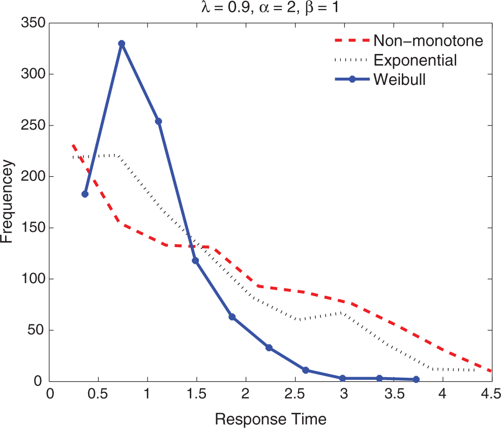
Illustration of response time distributions under different shapes of baseline hazard.

The three-parameter logistic model is used for generating item responses. Item discrimination and difficulty parameters are simulated from $a ~ U (1, 2.5)$ , $b ~ N (0, 1)$ , item pseudo-guessing parameter is simulated from $c ~ U (0, 0.2)$ . Examinees’ latent trait $(θ, τ)$ is drawn from a bivariate normal distribution with mean $μ = [0, 0]$ and covariance matrix $σ = [1, 0.5; 0.5, 1]$ . The regression parameter is drawn from $β ~ U (0.5, 1.5)$ . To implement the Bayesian MCMC algorithm, chains of length 4,000 with an initial burn-in period 1,000 are chosen. There were 10 replications for each simulation condition. Item and examinee parameters for each replication are generated separately.

4.2. Results

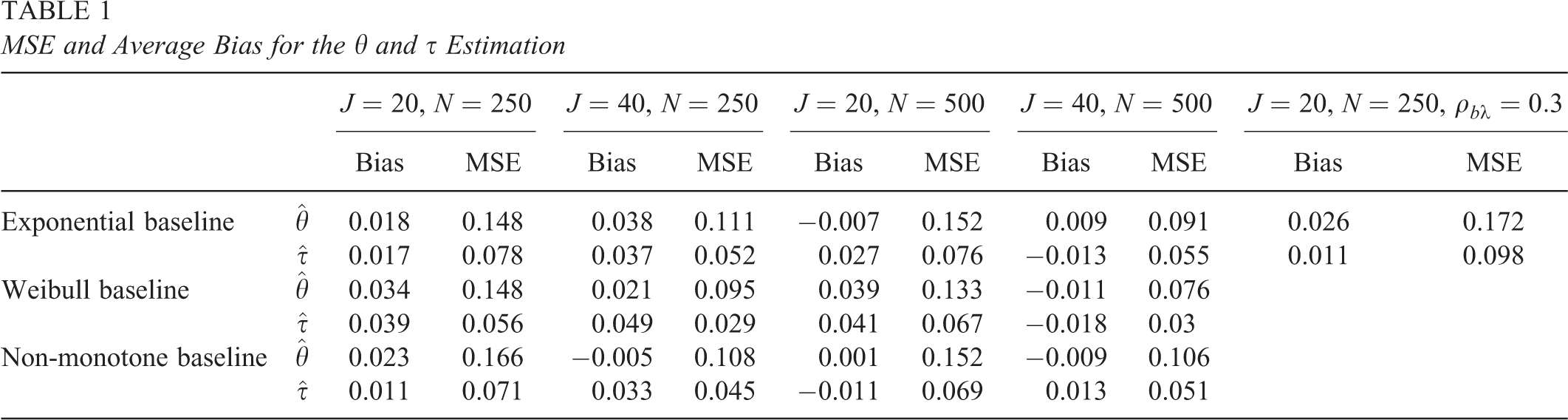
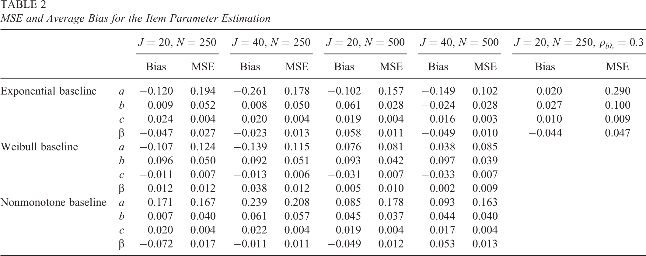
The Markov chain for each parameter appears to reach equilibrium and has small autocorrelations beyond the first couple of lags. Mean squared error (MSE) and average bias are calculated to check how close the estimated parameters were to their true values. Table 1 presents the MSE and bias of θ and τ for the 12 simulation conditions. All values are averaged over all examinees and all replications within a simulation condition. Table 2 tabulates the MSE and average bias for item parameters, including β and a, b, and c. Notice that the true value of $σ_{θ τ}$ across all conditions is 0.5. We report the final estimates of correlation term in Table 3, the values are calculated from the 10 replications. Please ignore the last two columns of each table for the moment.

Table 1

MSE and Average Bias for the θ and τ Estimation

		J = 20, N = 250		J = 40, N = 250		J = 20, N = 500		J = 40, N = 500		J = 20, N = 250, $ρ_{b λ} = 0.3$
		Bias	MSE	Bias	MSE	Bias	MSE	Bias	MSE	Bias	MSE
Exponential baseline	$\hat{θ}$	0.018	0.148	0.038	0.111	−0.007	0.152	0.009	0.091	0.026	0.172
	$\hat{τ}$	0.017	0.078	0.037	0.052	0.027	0.076	−0.013	0.055	0.011	0.098
Weibull baseline	$\hat{θ}$	0.034	0.148	0.021	0.095	0.039	0.133	−0.011	0.076
	$\hat{τ}$	0.039	0.056	0.049	0.029	0.041	0.067	−0.018	0.03
Non-monotone baseline	$\hat{θ}$	0.023	0.166	−0.005	0.108	0.001	0.152	−0.009	0.106
	$\hat{τ}$	0.011	0.071	0.033	0.045	−0.011	0.069	0.013	0.051

Table 2

MSE and Average Bias for the Item Parameter Estimation

		J = 20, N = 250		J = 40, N = 250		J = 20, N = 500		J = 40, N = 500		J = 20, N = 250, $ρ_{b λ} = 0.3$
		Bias	MSE	Bias	MSE	Bias	MSE	Bias	MSE	Bias	MSE
Exponential baseline	a	−0.120	0.194	−0.261	0.178	−0.102	0.157	−0.149	0.102	0.020	0.290
	b	0.009	0.052	0.008	0.050	0.061	0.028	−0.024	0.028	0.027	0.100
	c	0.024	0.004	0.020	0.004	0.019	0.004	0.016	0.003	0.010	0.009
	β	−0.047	0.027	−0.023	0.013	0.058	0.011	−0.049	0.010	−0.044	0.047
Weibull baseline	a	−0.107	0.124	−0.139	0.115	0.076	0.081	0.038	0.085
	b	0.096	0.050	0.092	0.051	0.093	0.042	0.097	0.039
	c	−0.011	0.007	−0.013	0.006	−0.031	0.007	−0.033	0.007
	β	0.012	0.012	0.038	0.012	0.005	0.010	−0.002	0.009
Nonmonotone baseline	a	−0.171	0.167	−0.239	0.208	−0.085	0.178	−0.093	0.163
	b	0.007	0.040	0.061	0.057	0.045	0.037	0.044	0.040
	c	0.020	0.004	0.022	0.004	0.019	0.004	0.017	0.004
	β	−0.072	0.017	−0.011	0.011	−0.049	0.012	0.053	0.013

Table 3

Mean and Standard Deviation for the Integrated Absolute Difference Between $H_{0} (t)$ and Breslow Estimator and Mean of $ρ_{θ τ}$

		J = 20, N = 250		J = 40, N = 250		J = 20, N = 500		J = 40, N = 500		J = 20, N = 250, $ρ_{b λ} = 0.3$
		M	SD	M	SD	M	SD	M	SD	M	SD
Exponential baseline	$d_{j}$	1.321	0.983	1.407	1.051	1.152	0.791	0.910	0.732	1.471	1.182
Exponential baseline	$ρ_{θ τ}$	0.507		0.491		0.519		0.485		0.521
Weibull baseline	$d_{j}$	1.980	1.69	1.449	1.238	1.471	1.131	1.503	1.219
Weibull baseline	$ρ_{θ τ}$	0.475		0.491		0.519		0.513
Nonmonotone baseline	$d_{j}$	1.296	0.934	0.994	0.841	0.918	0.643	0.899	0.651
Nonmonotone baseline	$ρ_{θ τ}$	0.511		0.466		0.492		0.491

For the log hazard ratio regression parameter β, the estimation is quite accurate in general, as indicated by the small MSE in Table 2. There is an apparent trend that increasing the population size reduces the MSE of β. The results also show that no matter which shape the baseline hazard takes, the model can always be accurately recovered. Increasing the test length reduces the MSE of τ and θ. Figure 2 shows the true and estimated cumulative baseline hazards. Here we only present the results for $J = 20$ and $N = 250$ under one replication because the other conditions are alike. The Breslow estimator appears to reconstruct the baseline cumulative hazard functions well under all three different shapes except at the right boundaries. The possible reason is at the right boundary, the size of the risk set is very small and thus the hazard estimation may be inflated. But considering only a small portion of examinees will have extreme RTs, this inflation is tolerable. To further quantify the discrepancy between the true and estimated cumulative hazard, we calculate the integrated absolute different between the true $H_{0 j} (t)$ and the Breslow estimator for the jth item

Figure 2.

True and estimated cumulative baseline hazard for different shapes of baseline hazard.

Figure 2.

continued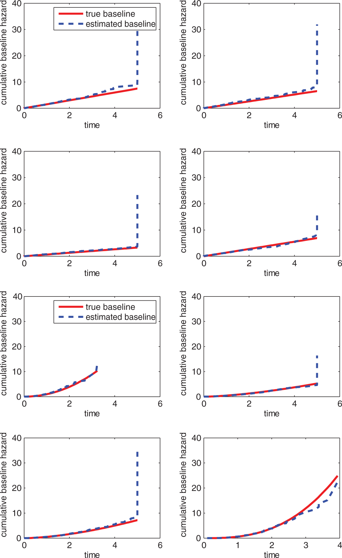

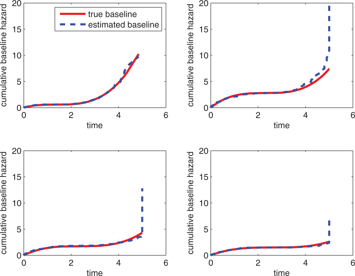
d_{j} = \int | H_{0 j} (t) - {\hat{H}}_{0 j} (t) | d t .

The mean and standard deviation of $d_{j}$ are reported in Table 3. In general, the value of $d_{j}$ is small indicating that the unknown cumulative hazard can be correctly recovered. The mean of $d_{j}$ decreases when the number of examinees increases, and the magnitude of mean $d_{j}$ is comparable across different shapes of baseline hazard, although $d_{j}$ tends to be slightly smaller under nonmonotone baseline condition. Considering that the true correlation between θ and τ is 0.5 in all cases, the ${\hat{ρ}}_{θ τ}$ is estimated accurately, as shown in Table 3.

4.3. Study 2

This study is designed to show that even if the item parameters have some moderate correlation, especially between item time intensity and item difficulty parameters, the proposed algorithm can still generate satisfactory results, with the item covariance matrix unestimated. As an illustration, we only consider the exponential model, in which the baseline hazard $λ_{j}$ is negatively correlated with the item difficulty $b_{j}$ to produce a positive correlation between item time intensity and item difficulty. Specifically, λs and bs are generated from bivariate normal with mean [1,0], and covariance matrix $[1, ρ_{λ b}; ρ_{λ b}, 1]$ , with two levels of $ρ_{λ b} = 0, 0.3$ . All the rest of the parameters are simulated in the same fashion as in simulation Study 1. The MSE and average bias for all parameters with $ρ_{λ b} = 0, 0.3$ are presented in the last two columns of Tables 1 and 2. When $ρ_{λ b} = 0$ , the results are very close to the results from simulation Study 1, and they are omitted here. As one can tell, with the increased correlation of $ρ_{λ b}$ , the estimation errors only slightly inflate, but they are still acceptable. Because the item covariance matrix will not influence our conclusion about the data, the second-level model on the item covariance matrix can be ignored to simplify the model estimation.

5. Empirical Example

This model is applied to a data set from a large scale high-stakes computerized adaptive test. The original data set is comprised of 21,444 examinees and 620 multiple choice items in total. The item 3PL parameters were precalibrated and were assumed known in this analysis. The default test length is 37, but the number of items that each examinee answers ranges from 25 to 37. Because of the computerized adaptive version, each item is answered by different sets of examinees, and the number of examinees taking each item rangs from 6 to 489. We randomly sample 3,000 examinees from this population for analysis. However, we delete 319 examinees because their RTs are not recorded; we further delete 548 examinees because their total RTs are either too long (longer than 75 minutes) or because they fail to finish the whole test (i.e., test length is shorter than 37). Longer than 75 minute tests occur because some examinees take the test under nonstandard “accommodation” settings. The resulting 2,061 observations are used in the analysis. The original RTs are recorded in a millisecond scale, and for ease of calculation, we rescale the RTs to the “minute” scale by dividing each RT record by $60, 000.$ The posterior distributions for the item and person parameters are approximated using the MCMC algorithm described earlier. The priors are specified in section 3.2.1.

To show that the new semiparametric model fits the empirical data better than the more restrictive parametric models, we consider three alternative parametric models: (1) the exponential model, with hazard function $h_{i j} (t | τ_{i}) = λ_{j} exp (β_{j} τ_{i})$ ; (2) the Weibull model, with hazard function $h_{i j} (t | τ_{i}) = γ_{j} (λ_{j} t)^{γ_{j} - 1} exp (β_{j} τ_{i})$ ; and (3) the lognormal model, with the RT density expressed as $f (t_{i j}) = \frac{α_{j}}{t_{i j} \sqrt{2 π}} exp {- \frac{1}{2} [α_{j} (log t_{i j} - (β_{j} - τ_{i}))]^{2}}$ . Different from the previous parameterizations, α functions as a discrimination parameter that corresponds to the discrimination power of an item in differentiating two examinees with different speed parameters; β indicates the time intensity of an item. These three models replace the Cox PH model in the hierarchical framework. The MCMC algorithm is employed for model estimation. But instead of using partial likelihood, the traditional likelihood for RTs (for the first two models for instance, $f (t) = h (t) exp {- \int_{0}^{t} h (s) d s}$ ) is used. The parameters for the baseline hazard, such as λ and γ, are updated in separate chains in the MCMC method. For the lognormal model, the complete algorithm introduced in van der Linden (2007) is used. In the lognormal model, van der Linden imposes a covariance structure on item parameters, and the covariance structure is estimated from the real data as well.

5.1. Model Selection

Model fit is checked via the three approaches introduced above. We first check the global fit of the semiparametric model against the parametric models, as shown in Figure 3a. This figure presents the cumulative distribution of the predictive probabilities for the observed RTs in Equation 10 for all person–item combinations in the data set. The data set is large enough (55,500 data points) to expect the empirical distribution to coincide with the identity line. The impression from Figure 3a is that the semiparametric model fits the data much better than the lognormal model and Weibull model, and the most restricted exponential model displays worst fit. Although the lognormal model does not show a good fit, one potential useful result from the lognormal model is that the covariance matrix on item parameters have all off-diagonal elements within the range of [−0.1, 0.05]. This indicates that the item parameters are nearly independent, although this conclusion should be made with caution because of the misfit of the model.

Figure 3.

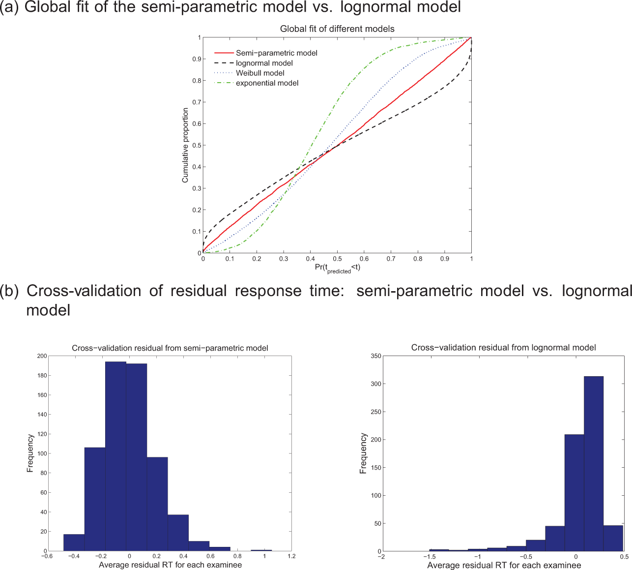
Diagnostic plots for different models.

Model fit is further checked by cross-validation, and a comparison is conducted between the semiparametric model and the lognormal model. A new independent sample of 1,500 examinees is drawn from the original data set, and 432 examinees are excluded due to the same criterion mentioned earlier. The remaining 1,068 examinees form the cross-validation sample.

The residual in Equation 11 is calculated for each examinee in the cross-validation sample. Observe that in the calibration sample, there are 30 items that are answered by fewer than 20 examinees, and the parameter estimations for those items are expected to be less accurate and reliable. Therefore, rather than presenting the mean residual RTs for every examinee in the cross-validation sample, we decide to only present the residuals calculated from those examinees who answered items with item parameters estimated from a sample size larger than 40 in the calibration sample. The cross-validation residuals are presented in Figure 3b. Apparently, both models generate acceptably small residuals. The lognormal model, which has fewer parameters, tends to generate smaller residuals for a larger number of people, as indicated by more than 220 examinees with residuals falling into the range of [−0.05, 0.05], versus 190 from semiparametric model. On the other hand, the semiparametric model is more flexible to capture various shapes of RT distributions, some of which might be hard to represent by the lognormal distribution. Accordingly, the lognormal model is a poor fit for certain items and yields a greater proportion of the more extreme cross-validation residuals.

To show the item-level fit of the semiparametric model, we draw the distribution plot of $ϵ_{i j}$ defined in Equation 13 against the extreme-value distribution. Similar to the Q-Q plot, points tightly along a line indicate a good fit. We find that the majority of the items showed pretty good fit. Figure 4 presents the fit plots for 6 items under the new model. The 3 items on the left are the ones with the best fit and the 3 items on the right are the ones with the worst fit. All these 6 items are answered by more than 200 examinees and have reliable parameter estimates. As demonstrated by Figure 4, some of the items are fitted quite well, but some are not. This might be because the current model assumes that the hazards are proportional, which might be violated for some items. This suggests the need for a more general model that relaxes such an assumption, for example, the linear transformation model (Cuzick, 1988; Wang, Chang, & Douglas, 2012).

Figure 4.

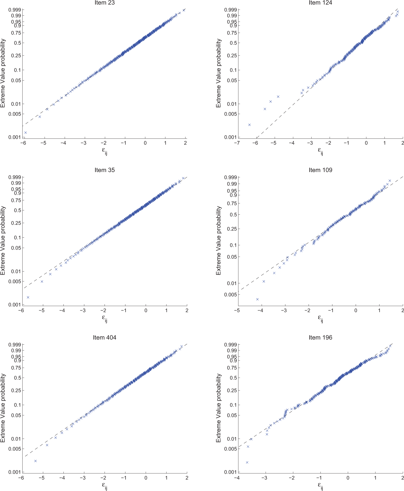
Item-level residuals for 6 items.

5.2. Parameter Estimates

Because the model fit checking indicates that the semiparametric model fits the data best, in this subsection, we will only report the model calibration result from this new model. The correlation between τ and θ is as high as .71, meaning that more capable examinees tended to answer the items faster. The average value of ${\hat{θ}}_{i}$ , averaging over 2,036 examinees, is .66; the average value of ${\hat{τ}}_{i}$ is .005. The posterior mean of $σ_{θ}^{2}$ is 1.40 and of $μ_{θ}$ is .65. To show how examinees’ RT changes with the latent speed, we provide histograms of ${\hat{β}}_{j}$ , as shown in Figure 5, and the mean value of ${\hat{β}}_{j}$ , averaging over all 620 items, is .27. Of the 620 items, there are around 120 items with ${\hat{β}}_{j}$ close to 0, which indicates that for those items, there is no clear trend between examinees’ speed and actual RT. This is a typical phenomenon yielded by the “restriction of range in correlation.” In other words, these items are only exposed to a certain group of examinees with a small range of abilities or speed parameters rather than a representative group. For instance, if a relatively difficult item is given to a representative group, then ${\hat{β}}_{j}$ will most likely be positive; however, if only high-ability examinees answer the item, within the restricted sample, the ${\hat{β}}_{j}$ estimate might be close zero. To further verify this possibility, we explore 2 items that have very small ${\hat{β}}_{j}$ , against 2 items with large ${\hat{β}}_{j}$ in Figure 6. The items with small ${\hat{β}}_{j}$ were given to examinees with high abilities yielding narrower ability ranges.

Figure 5.

$\hat{β}$ distribution estimated from the semiparametric model.

Figure 6.

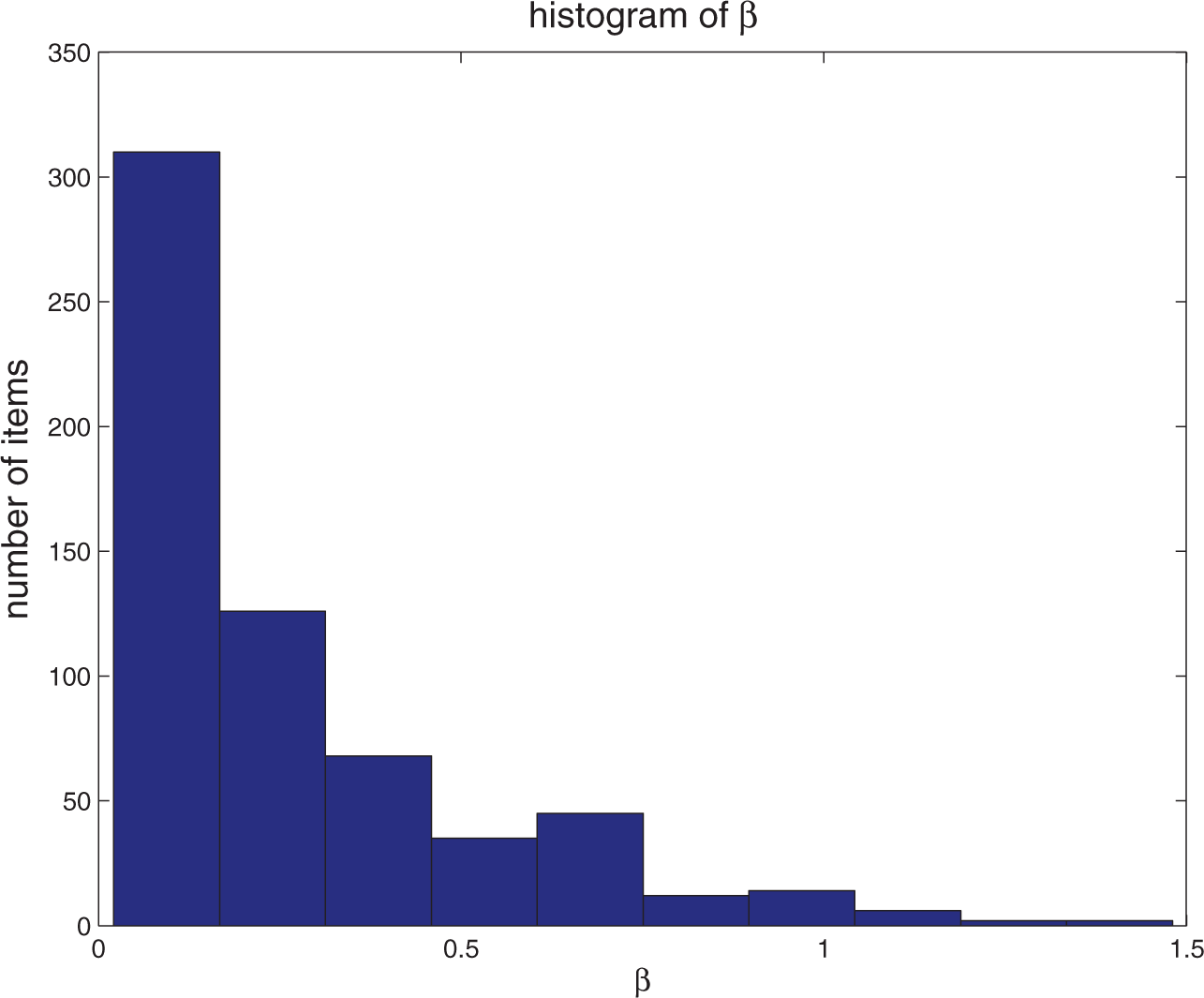
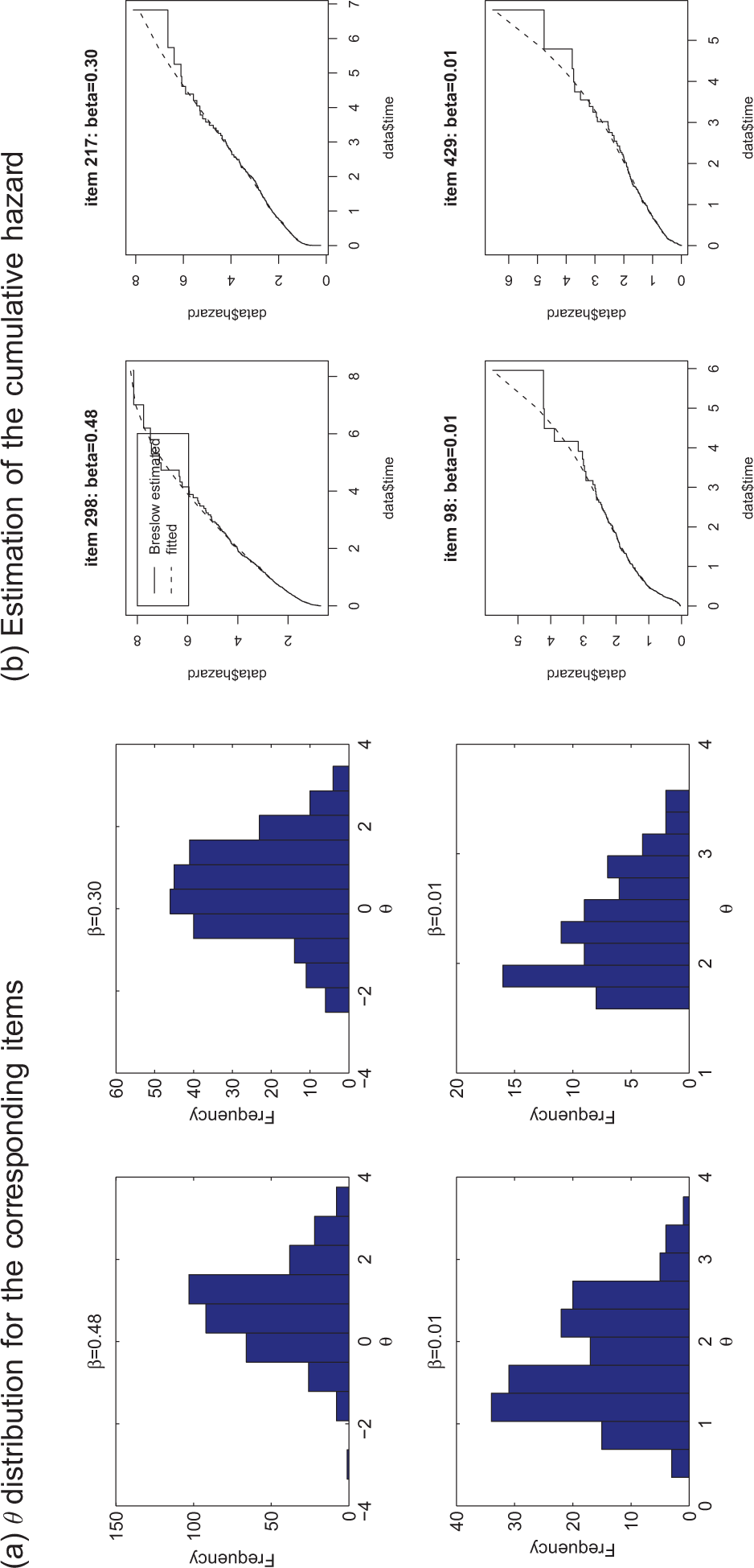
Illustration of the RT histogram, cumulative baseline hazard, and examinees’ ability distribution for 4 items.

The baseline cumulative hazards calculated from the Brewslow estimator are also provided in Figure 6b. When fitting the B-spline, the degree of the B-spline basis was set to be 3, and three inner knots were chosen to construct the basis. R functions bs in “splines”package were used to carry out the B-spline fitting, and function lm was used to regress the B-spline bases on the Breslow estimation results through linear models. The B-spline curve is plotted against the Breslow estimator for the 4 items, as presented in Figure 6b. It shows that the B-spline curves fit well with the points estimated from the nonparametric Breslow estimator, and therefore, we can largely reduce the number of parameters needed to adequately recover the entire cumulative baseline hazard estimate.

5.3. Further Model Diagnostics

Two key assumptions of the model are the local independence and stationarity assumptions. Van der Linden and Glas (2010) proposed a score test statistic (also known as Lagrange Multiplier [LM] test statistic) to check the local independence of responses and RTs. The same idea is applied in this study and is briefly presented below and in Appendix B. First, the assumption of conditional independence between RT and response accuracy can be equivalently expressed as

f (t_{i j} | y_{i j}, τ_{i}) = f (t_{i j} | τ_{i}), y_{i j} = 0, 1

for examinee i and item j. If this assumption is violated, the RT model could be modified as

h_{j} (t_{i j}) = h_{0 j} (t) exp (β_{j} τ_{i} + λ_{j} y_{i j}),

thus the assumption check reduces to check the significance of $λ_{j}$ for item j. The null hypothesis would be

H_{0} : λ_{j} = 0,

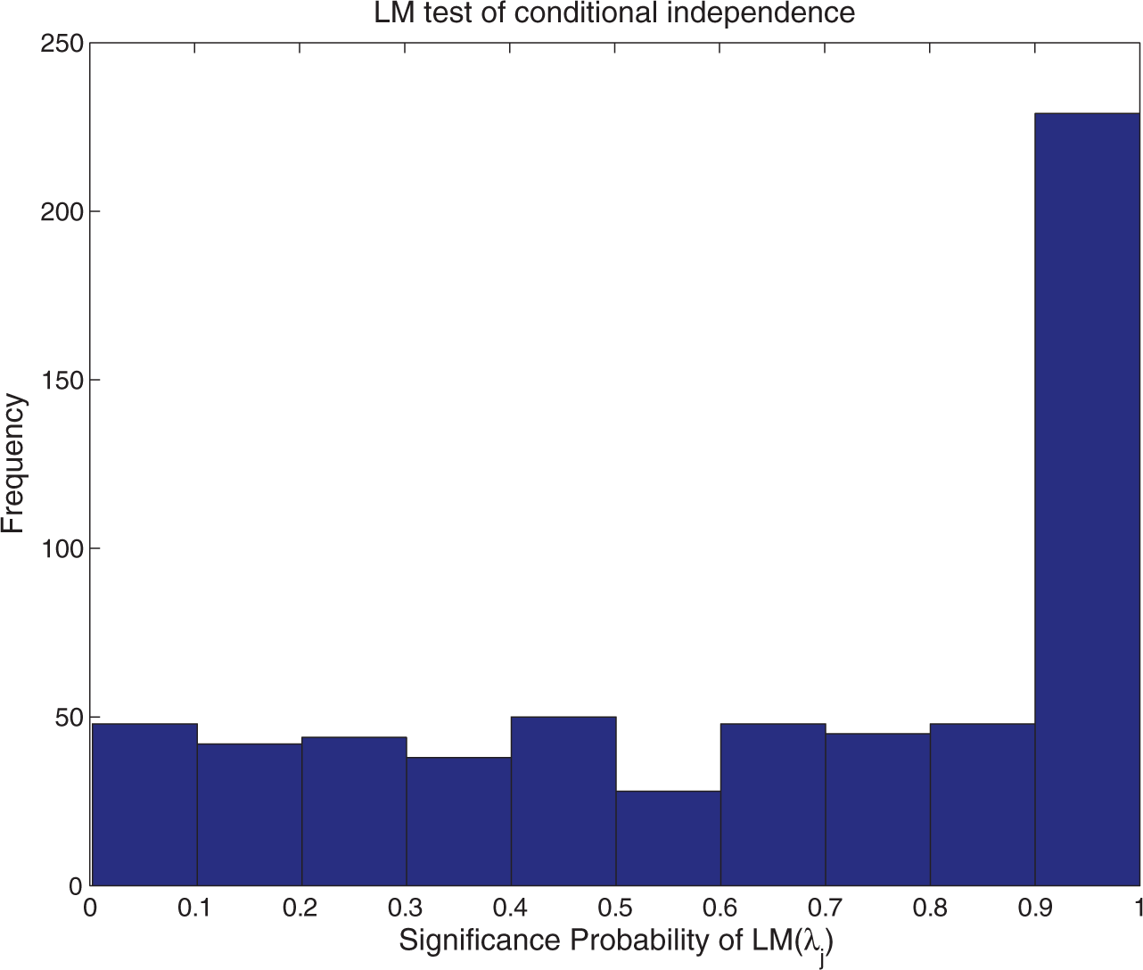
whereas the alternative hypothesis is $H_{1} : λ_{j} \neq 0$ . For the 620 items in the item bank, the $L M (λ_{j})$ s are presented in Figure 7. Only 43 items have probabilities significant at 5% level. This supports our conclusion that this local independence assumption was satisfied.

Figure 7.

Lagrange multiplier probability for conditional independence.

The stationary assumption claims that examinees’ speed and ability are constant during the test. While constant ability is standard in item response modeling, the constant speed assumption needs to be checked. For examinee i, we calculated the residual RTs as

r_{i j} = {\tilde{t}}_{i j} - t_{i j} = \int exp [- exp {\hat{β}}_{j} {\hat{τ}}_{i} {\hat{H}}_{0 j} (t)] d t - t_{i j},

for $j = 1, 2, . . ., 37$ . We then conducted the Wald–Wolfowitz RUNS test (Wald & Wofowitz, 1940) on residual RTs for each examinee separately. The null hypothesis is that the residuals on different items were independent, that is, there was no item position effect and the examinee’s speed can be viewed as a constant. Of the 2,036 test takers in the calibration sample, only 93 were rejected, which implies that the stationarity assumption might hold. In addition, as in van der Linden et al. (2007), we plotted the residual RT against item position for four randomly chosen examinees in Figure 8. If the stationary assumption holds, the residual should fluctuate around 0 along the tests. But as one can see, for some examinees, the residuals were uniformly negative at the beginning and positive toward the end. That means, they worked somewhat slower than expected at the beginning of the test and compensated toward the end. Our statistical analysis of this conflicted somewhat with our graphical analysis, but we do believe a slight position effect exists.

Figure 8.

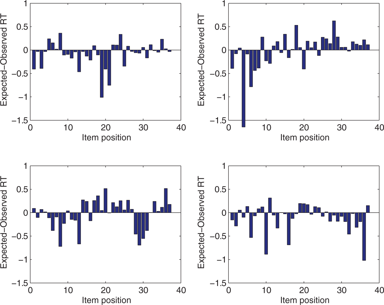
Mean residual times on the items as a function of their position in the test: four selected examinees.

6. Discussion and Future Work

Since the 1972 publication of Cox’s seminal article on statistical models for lifetime data, survival methods, especially those for continuous time data, have enjoyed increasing popularity in a variety of disciplines ranging from medicine and industrial testing to economics and sociology. RT analysis, a specific research topic in educational measurement, will also benefit from advances in survival methods. In fact, the semiparametric modeling approach in survival analysis opens another avenue for RT modeling. Most recently, Ranger and Ortner (2011) proposed to use Cox model in RT modeling, and they replaced the observed covariates in the Cox model with the test takers’ latent speed. In this article, we proposed to insert their model in the two-level framework proposed by van der Linden (2007) such that the RT and response accuracy are modeled simultaneously. This model hinges on the assumption that examinees’ latent speed determine their RTs directly. This new model assigns a separate speed parameter τ to account for the individual differences in speed, while allowing τ to be correlated with θ at population level. The hierarchical framework (van der Linden, 2007) distinguishes the speed–accuracy trade-off within a person from the speed accuracy correlation across persons. Simulation studies show that the new model can be estimated accurately via a two-stage estimation method. One apparent advantage of the proposed model comes from its semiparametric nature. The nonparametric baseline hazard is flexible enough to accommodate different shapes of RT distributions in real data. Once the nonparametric baseline hazard is recovered by the Breslow estimator, we can further fit it either with a parametric form or with a curve generated by B-spline basis, depending upon the specific shapes of the baseline hazard. Also due to the nonparametric term, the new models subsume a variety of different models, such as the exponential regression model, the Weibull regression model and others.

The estimation method proposed in this article uses the partial likelihood function, which is motivated as resulting from integrating out the baseline cumulative hazard function with respect to a gamma process prior. Although Clayton (1991) also adopts a gamma process prior, he includes the cumulative baseline hazard as a “parameter” to be updated within each Markov chain. Sharef et al. (2010) advocated using B-splines on H ₀ and update it in MCMC as well. An apparent advantage of their approaches is that inference can be made on the baseline hazard. However, with a somewhat complicated posterior distribution encountered here, it seems more beneficial to use a divide-and-conquer approach. That is, treat the nonparametric baseline hazard as a nuisance parameter and integrate it out first, and once the parameters are accurately calibrated, estimate the nonparametric hazard secondly.

A future direction is to introduce additional covariates in the model, such as examinees’ demographic information, to better explain the RT variance. A survival model that is suitable for such a purpose is

h_{j} (t_{i j} | τ_{i}, Z_{i}) = h_{0 j} (t_{i j}) exp (β_{j} τ_{i} + γ_{j}^{'} Z),

where $Z_{i} = (z_{i 1}, . . ., z_{i p})$ represents the observed covariates, such as gender, educational background, social economic status, and such things. This extended model is also able to explain variation in speed between individuals that may be nested within groups.

The real-data example shows that the proposed semiparametric model tends to fit the data better than the more restricted lognormal model, or other parametric models. One limitation of this study is that we only compared the performance of the semiparametric model with simpler parametric models. In the future, more flexible parametric models, such as the Box-Cox normal model (Klein Entink et al., 2009) or the generalized linear model with flexible link function (Ranger & Kuhn, 2011) should be considered as potential alternative models. Further studies should also confirm the applicability of the new model for other types of test data (such as nonadaptive achievement tests). Another future direction is to further break down the latent speed parameter τ into different information processing components, because different examinees might employ different strategies when solving an item. Response caution also plays an important role in examinees’ processing speed (van der Mass, Molenaar, Maris, Kievit, & Borsboom, 2011).

The ultimate goal of RT research is to further enhance the quality of tests and to improve the estimation accuracy of the examinees’ abilities. A test’s quality includes test fairness, test efficiency, and so on. In particular, concerning test fairness, RTs allow us to formulate constraints on item selection (in adaptive tests) or test assembly (in linear form tests) that guarantee the multiple forms of a test to be equally speeded. In our modeling approach here, $\int_{0}^{\infty} S_{j} (t | β, τ, h_{0}) d t$ is the expected time to answer the jth item, and upon knowing this, the constraint related to RTs can be easily incorporated in item selection through the weighted deviation model or the constraint weighted index. Concerning efficiency, observe that a highly informative item can be quite time consuming, so it has less practical value compared to an equally or somewhat less informative items that require less time to complete. Therefore, instead of maximizing the raw item information, we can maximize the item information per time unit. In other words, we select the m + 1 item based on

j_{m + 1} = max_{l} \{\frac{I_{l} ({\hat{θ}}^{m l e})}{\int S_{l} (t | {\hat{β}}^{m l e}, {\hat{τ}}^{m l e}, {\hat{h}}_{0}) d t} : l \in R_{m}\},

where R_m denotes the available items in the item pool and $I_{l} ({\hat{θ}}^{m l e})$ denotes the regular Fisher item information (Fan et al., 2012). In this way, more information is accumulated in the allowed time. Besides the above two possible applications, RT information can be used in addition to responses for ability estimation during the course of an adaptive test.

Footnotes

Appendix A

For the ith test taker, his or her responses and RTs are denoted by $Y_{i} = (Y_{1 i}, \dots, Y_{J i})^{'}$ , and $T_{i} = (T_{1 i}, \dots, T_{J i})^{'}$ , respectively. To perform the sampling for parameters with support on the entire real line, we use normal proposal distributions with mean equal to the current estimation and variance chosen to give a Metropolis acceptance rate of between 25% and 40%. For parameters with support not on the real line, we first transform them to the real line and then sample them from normal proposal distribution.

Appendix B

Similar to van der Linden and Glas (2010), we assumed the item parameters, including $β_{j}$ and $h_{0 j}$ , were precalibrated. Thus, for a given item, the parameters that need to be estimated are $τ = (τ_{1}, . . ., τ_{N})$ and $λ_{j}$ . The likelihood can be rewritten as

l (τ, λ_{j}) = log {\prod_{i = 1}^{N} [f (t_{i j} | τ_{i}, β_{j}, λ_{j}) \prod_{l = 1; l \neq j}^{J} f (t_{i j} | τ_{i}, β_{l})]}

where

f (t_{i j} | τ_{i}, β_{j}, λ_{j}) = H_{j} (t_{i j}) {exp}^{β_{j} τ_{i} + λ_{j} u_{i j}} {exp}^{- {exp}^{β_{j} τ_{i} + λ_{j} u_{i j}} H_{j} (t_{i j})},

and

f (t_{i l} | τ_{i}, β_{l}) = H_{j} (t_{i j}) {exp}^{β_{l} τ_{i}} {exp}^{- {exp}^{β_{l} τ_{i}} H_{j} (t_{i j})} .12 p t

For item j, the LM statistic is constructed as

L M (λ_{j}) = \frac{h (λ_{j})^{2}}{h (λ_{j}, λ_{j}) - H (τ, λ_{j})^{'} H (τ, τ)^{- 1} H (τ, λ_{j})} |_{τ = \hat{τ}, λ_{j} = 0},

where $H (τ, τ)$ is an $n_{j} \times n_{j}$ diagonal matrix with $n_{j}$ denoting the number of examinees answering the jth item. By plugging in the likelihood function in Equation B1 into B2, we have

\begin{aligned} - H^{i i} (τ, τ) = - β_{j}^{2} H_{j} (t_{i j}) exp (β_{j} τ_{i} + λ_{j} u_{i j}) - \sum_{l = 1; l \neq j}^{J} β_{l}^{2} H_{j} (t_{i j}) exp (β_{l} τ_{i}) \\ - h (λ_{j}) = \sum_{i = 1}^{n_{j}} u_{i j} - \sum_{i = 1}^{n_{j}} H_{j} (t_{i j}) exp (β_{j} τ_{i} + λ_{j} u_{i j}) u_{i j} \\ - h (λ_{j}, λ_{j}) = - \sum_{i = 1}^{n_{j}} u_{i j}^{2} H_{j} (t_{i j}) exp (β_{j} τ_{i} + λ_{j} u_{i j}) \\ - H^{i} (τ, λ_{j}) = - H_{j} (t_{i j}) exp (β_{j} τ_{i} + λ_{j} u_{i j}) β_{j} u_{i j} . \end{aligned}

Declaration of Conflicting Interests

The authors declared no potential conflicts of interest with respect to the research, authorship, and/or publication of this article.

Funding

The authors disclosed receipt of the following financial support for the research, authorship, and/or publication of this article: This work was funded by a grant from the National Science Foundation, NSF-MMS 0960822.

References

Anderson

P. K.

Borgan Gill

R. D.

Keiding

(1992). Statistical models based on counting processes. New York, NY: Springer.

Breslow

N. E.

(1972). Discussion of the paper by D. R. Cox. Journal of the Royal Statistical Society, Series B, 34, 216–217.

Bridgeman

Cline

(2004). Effects of differentially time-consuming tests on computer-adaptive test scores. Journal of Educational Measurement, 41, 137–148.

Cai

Hyndman

Wand

(2002). Mixed model-based hazard estimation. Journal of Computational and Graphical Statistics, 11, 784–798.

Clayton

Cuzick

(1985). Multivariate generalizations of the proportional hazards model (with discussion). Journal of the Royal Statistical Society, Series A, 148, 82–117.

Clayton

D. G.

(1991). A Monte Carlo method for Bayesian inference in frailty models. Biometrics, 48, 61–72.

Cox

D. R.

(1972). Regression models and life tables. Journal of the Royal Statistical Society, Series B, 34, 187–202.

Cuzick

(1988). Rank regression. The Annals of Statistics, 16, 1369–1389.

de Boor

C. A.

(1978). A practical guide to splines. New York, NY: Springer-Verlag.

10.

Doksum

K. A.

(1987). An extension of partial likelihood methods for proportional hazard models to general transformation models. The Annals of Statistics, 15, 325–345.

11.

Douglas

J. A.

Kosorok

M. R.

Chewning

B. A.

(1999). A latent variable model for discrete multivariate psychometric waiting times. Psychometrika, 64, 69–82.

12.

Fan

Wang

Chang

Douglas

(2012). Utilizing response time distributions for item selection in CAT, Journal of Educational and Behavioral Statistics, 37, 655–670.

13.

Friedman

(1982). Piecewise exponential models for survival data with covariates. Annals of Statistics, 10, 101–113.

14.

Shi

(1998). Monotone B-Spline smoothing. Journal of the American Statistical Association, 93, 643–650.

15.

Henschel

Engel

Holzel

Mansmann

(2009). A semiparametric Bayesian proportional hazard model for interval censored data with frailty effects. BMC Methological Research Methodology, 9, 9. doi:10.1186/1471-2288-9-9

16.

Gelman

Carlin

J. B.

Stern

Rubin

D. B.

(1995). Bayesian data analysis. London, England: Chapman and Hall.

17.

Gray

R. J.

(1994). A Bayesin analysis of institutional effects in a multicenter cancer clinical trial. Biometrics, 50, 244–253.

18.

Gustafson

(1997). Large hierarchical Bayesian analysis of multivariate survival data. Biometrics, 53, 230–242.

19.

Kalbfleisch

J. D.

(1978). Non-parametric Bayesian analysis of survival time data. Journal of Royal Statistical Society, Series B, 40, 214–221.

20.

Kalbfleisch

J. D.

Prentice

R.L.

(1973). Marginal likelihoods based on Cox's regression and life model. Biometrika, 60, 267–278.

21.

Klein Entink

R. H.

van der Linden

W. J.

Fox

J.-P.

(2009). A Box-Cox normal model for response times. British Journal of Mathematical and Statistical Psychology, 62, 621–640.

22.

Luce

R. D.

(1986). Response times: Their role in inferring elementary mental organization. New York: Oxford University Press.

23.

McCullagh

(1980). Regression models for ordinal data. Journal of the Royal Statistical Society, Series B, 42, 109–142.

24.

Patz

R. J.

Junker

B. W.

(1999). A straightforward approach to Markov Chain Monte Carlo methods for item response models. Journal of Educational and Behavioral Statistics, 24, 146–178.

25.

Posner

M. J.

Boies

S. J.

(1972). Components of attention. Psychological Review, 78, 391–408.

26.

Ranger

Kuhn

J. T.

(2011). A flexible latent trait model for response times in tests. Psychometrika, 77, 31–47.

27.

Ranger

Ortner

(2011). A latent trait model for response times on tests employing the proportional hazards model. British Journal of Mathematical and Statistical Psychology, 65, 334–349. DOI:10.1111/j.2044-8317.2011.02032.x

28.

Roskam

E. E.

(1997). Models for speed and time-limit tests. In van der Linden

W. J.

Hambleton

(Eds.), Handbook of modern item response theory (pp. 187–208). New York, NY: Springer.

29.

Rounder

J. N.

Sun

Speckman

P. L.

Zhou

(2003). A hierarchical Bayesian statistical framework for response time distributions, Psychometrika, 68, 589–606.

30.

Sargent

D. J.

(1998). A general framework for random effects survival analysis in the Cox proportional hazards setting. Biometrics, 54, 1486–1497.

31.

Schnipke

D. L.

Scrams

D. J.

(1997). Modeling response times with a two-state mixture model: A new method of measuring speededness. Journal of Educational Measurement, 34, 213–232.

32.

Schnipke

D. L.

Scrams

D. J.

(2002). Representing response time information in item banks. (LSAC Computerized Testing Report No. 97-09). Newton, PA: Law School Admission Council.

33.

Sharef

Strawderman

R. L.

Ruppert

Cowen

Halasyamani

(2010). Bayesian adaptive B-spline estimation in proportional hazards frailty models. Electronic Journal of Statistics, 4, 606–642.

34.

Singer

J. D.

Willett

J. B.

(1993). It’s about time: Using discrete-time survival analysis to study duration and the timing of events. Journal of Educational Statistics, 18, 155–195.

35.

Tate

M. W.

(1948). Individual differences in speed of response in mental test materials of varying degrees of difficulty. Educational and Psychological Measurement, 8, 353–374.

36.

Thissen

(1983). Timed testing: An approach using item response theory. In Weiss

D. J.

(Ed.), New horizons in testing (pp.179–203). New York, NY: Academic Press.

37.

Tierney

(1994). Markov chains for exploring posterior distributions (with discussion). Annals of Statistics, 22, 1701–1762.

38.

van der Linden

W. J.

(2007). A hierarchical framework for modeling speed and accuracy on test items. Psychometrika, 72, 287–308.

39.

van der Linden

W. J.

Breithaupt

Chuah

S. C.

Zhang

(2007). Detecting differential speededness in multistage testing. Journal of Educational Measurement, 44, 117–130.

40.

van der Linden

W. J.

Glas

C. A. W.

(2010). Statistical tests of conditional independence between responses and/or response times on test items. Psychometrika, 75, 120–139.

41.

van der Linden

W. J.

Guo

(2008). Bayesian procedures for identifying aberrant response-time patterns in adaptive testing. Psychometrika, 73, 365–384.

42.

van der Mass

H. L. J.

Molenaar

Maris

Kievit

R. A.

Borsboom

(2011). Cognitive psychology meets psychometric theory: On the relation between process models for decision making and latent variable models for individual differences. Psychological Review, 118, 339–356.

43.

Verhelst

N. D.

Verstralen

H. H. F. M.

Jansen

M. G.

(1997). A logistic model for time-limit tests. In van der Linden

W. J.

Hambleton

R. K.

(Eds.), Handbook of modern item response theory (pp. 169–185). New York, NY: Springer-Verlag.

44.

Wald

Wolfowitz

(1940). On a test whether two samples are from the same population. The Annals of Mathematical Statistics, 11, 147–162.

45.

Wang

Chang

Douglas

(2012). The linear transformation model with frailties for the analysis of item response times. British Journal of Mathematical and Statistical Psychology. doi:10.1111/j.2044-8317.2012.02045.x

46.

Wang

Hanson

B. A.

(2005). Development and calibration of an item respnse model that incorporates response time. Applied Psychological Measurement, 29, 323–339.

47.

Wenger

Gibson

(2004). Using hazard functions to assess changes in processing capacity in an attentional cuing paradigm. Journal of Experimental Psychology, 30, 708–719.

48.

Ying

Chang

(2005, April). Modeling response latencies for computerized adaptive tests. Paper presented at the annual meeting of the National Council on Measurement in Education, Montreal, Canada.