Conditional Optimal Design in Three- and Four-Level Experiments

Abstract

The precision of estimates of treatment effects in multilevel experiments depends on the sample sizes chosen at each level. It is often desirable to choose sample sizes at each level to obtain the smallest variance for a fixed total cost, that is, to obtain optimal sample allocation. This article extends previous results on optimal allocation to four-level cluster randomized designs and randomized block designs. It also introduces the idea of constrained optimal allocation, where the sample size at one or more levels is fixed by considerations other than cost or sampling variation. Explicit formulas are given for constrained optimal allocation in three- and four-level designs.

Keywords

cluster randomized trial multisite design randomized block design optimal design

Randomized experiments provide the best evidence about causal effects of educational interventions, products, or services (in this article, we refer to any of these as treatments). Consequently, there has been increasing emphasis on the use of randomized experiments in educational research. For example, the U.S. Institute of Education Sciences (IES) has encouraged its contractors and grantees to use randomized experiments in their evaluation designs whenever possible. Educational field experiments often use some form of group-based assignment to treatments (e.g., assigning whole classrooms or schools to the same treatment) because individual assignment is either practically infeasible, politically unacceptable, or (as in the case of treatments such as whole school reforms) theoretically impossible. Group assignment naturally gives rise to multilevel sampling designs in which a sample of groups, such as schools, yield multistage cluster samples. Often the sampling design involves more than two levels, such as in designs where the experimental sample consists of individuals nested within classrooms, which in turn are nested within schools, which themselves may be drawn from school districts. In fact, a survey of the designs used in IES-funded experiments from 2005 to 2008 (Spybrook & Raudenbush, 2009) found that the most common designs among the studies reviewed actually involved four levels of nesting.

In single-level experiments (such as those using completely randomized designs) analyzed by the analysis of covariance, the statistical power of tests for treatment effects and the precision of treatment effect estimates depend on sample size, effect size, and the proportion of variance explained by any covariates that may be used. However, in multilevel experiments, the statistical power of tests for treatment effects and the precision of treatment effect estimates also depend on how the sample size is allocated across levels of the design and the variance decomposition across levels of the design (usually summarized by the intraclass correlation structure). Thus, in multilevel experiments, it is possible for the same total sample size to give rise to vastly different statistical power or precision, depending on how the total sample is allocated across levels of the design. This raises the question of how to allocate sample across the levels of the design. One approach to this problem is to introduce a cost function that depends on sample size at each level and determine the design that produces the most efficient estimate of the treatment effect (or greatest statistical power) for a given fixed cost.

Raudenbush (1997) discussed optimal design in two-level cluster randomized experiments (with and without covariates). Raudenbush and Liu (2000) discussed optimal design in two-level experiments with randomized block designs (with and without covariates). These ideas were extended to three-level designs by Moerbeek, van Breukelen, and Berger (2000); Liu (2003); and Konstantopoulos (2009, 2011) for both cluster randomized (i.e., designs with treatment assignment to units at the highest level of the design) and randomized block designs (i.e., designs where treatment assignment is made to units at other levels than the highest). Liu also considered unequal costs and unequal allocation of clusters between experimental and control conditions. To the best of our knowledge, there is no published account of optimal allocation in four-level designs. A review of the optimal design literature for multilevel models is given in chapter 6 of Berger and Wong (2009).

In two-level designs, the optimal allocation problem is to determine the number of units at the individual level within each cluster that leads either to the most efficient estimate of the treatment effect or to the greatest statistical power for a given fixed cost. These optimal allocation computations are often useful because they suggest much smaller sample sizes at Level 1 than investigators might think are necessary, suggesting where efficiencies can be obtained. These optimal allocations depend on assumed values of intraclass correlations (and effectiveness of covariates at explaining variation at various levels of the design). Korendijk, Moerbeek, and Maas (2010) have studied the robustness of optimal allocations to incorrect assumptions about intraclass correlation and found that they are reasonably robust.

In three- or four-level designs, the number of units at some levels may be constrained for reasons other than efficiency. For example, a design may be planned, so that it has exactly two classrooms per school to ensure replication across teachers within schools. Alternatively, a design may be planned, so that it tests all of the students in a classroom to minimize disruption. In either case, the number of units chosen at one level may not be optimal in the sense of cost efficiency, but it may be desirable to determine the allocation of the sample at other level/levels in a way that is optimal, given this constraint.

The purpose of this article is to extend optimal design ideas to four-level designs for both hierarchical and randomized block designs. We also provide results for constrained optimal designs in which the sample size at one or more levels is fixed and the problem is to obtain the optimal allocation of sample sizes at the other levels.

Why Constrained Optimal Design Can Be Useful

To see why constrained optimal design can be useful, consider the example of an evaluation of a program (Schoolwide Positive Behavioral Support) that is being designed by the U.S. IES. The senior author served on the technical working group advising on the design of this randomized experiment. The treatment is inherently a school-level intervention, but it involves considerable support from district personnel. Members of the technical working group were concerned that, because the district personnel served many schools in the district, there would be potential for contamination between treatment and control group schools within the same district. Therefore, they recommended that assignment of treatments take place at the district level in a three-level design, with districts assigned to treatments, schools nested within districts, and students nested within schools (a three-level hierarchical or cluster randomized design).

Using multiple states in the experiment would require the administration of common achievement measures within the study, which would increase costs. Consequently, it was recommended that there were advantages in conducting the evaluation within a single state, so that the state assessment could be used to provide the achievement test data. A second advantage of conducting the evaluation within a single state is that information about intraclass correlations based on state assessment data is available. We use the state of Florida as an example.

In a situation like this, available cost and intraclass correlation data could be used to determine the optimal number of Level 1 units (students) per Level 2 unit (school) and the number of Level 2 units per Level 3 unit (district). However, the IES wanted to use only p = 2 schools per district. The question is how best to obtain an efficient design (a design that has the smallest variance of the treatment effect estimate), given the constraint of p = 2 schools per district and a fixed cost.

Four-Level Hierarchical Designs

In this section, we describe the models underlying the results presented in this article. We first describe the four-level model and then show how these can be simplified to three-level and two-level situations.

Model and Notation

Suppose that there is a four-stage cluster sampling design with 2m clusters (Level 4 units) with m clusters assigned to each treatment, each cluster has r subclusters (Level 3 units), and each subcluster has p sub-subclusters (Level 2 units) of size n. Let Y_ijkl be the lth observation in the kth sub-subcluster of the jth subcluster of the ith cluster. If there is a covariate W at Level 4, a covariate U at Level 3, a covariate Z at Level 2, a covariate X at Level 1, and a treatment indicator T, all of which are group mean centered, then the model is

\begin{aligned} Y_{i j k l} & = μ + β_{1} T_{i} + β_{2} W_{i} + γ U_{i j} + δ Z_{i j k} + π X_{i j k l} + ζ_{i} + η_{i j} + ξ_{i j k} + ϵ_{i j k l}, \\ i & = 1, \dots, 2 m; j = 1, \dots, r; k = 1, \dots, p; l = 1, \dots, n . \end{aligned}

The fixed effects are the grand mean μ, the covariate-adjusted treatment effect β₁, the effect of the Level 4 covariate β₂, the effect of the Level 3 covariate γ, the effect of the Level 2 covariate δ, and the effect of the Level 1 covariate π. The random effects at Level 4 (the ζ _i ), Level 3 (the η _ij ), Level 2 (the ξ _ijk ), and Level 1 (the ∊ _ijkl ) are assumed to be independently normally distributed with zero means and variances $σ_{A 4}^{2}, σ_{A 3}^{2}, σ_{A 2}^{2}, a n d σ_{A 1}^{2}$ , respectively. Here the A in the subscript of the residual variances refers to the fact that the model includes covariates, so that the variances are adjusted for the covariates; the variances in a model without covariates would be denoted by $σ_{4}^{2}, σ_{3}^{2}, σ_{2}^{2}, a n d σ_{1}^{2}$ , respectively. The covariate outcome correlations are defined in terms of the adjusted and unadjusted variances as $P_{1}^{2} = 1 - {\overset{ˉ}{P}}_{1}^{2} = 1 - σ_{A 1}^{2} / σ_{1}^{2}$ , $P_{2}^{2} = 1 - {\overset{ˉ}{P}}_{2}^{2} = 1 - σ_{A 2}^{2} / σ_{2}^{2}$ , $P_{3}^{2} = 1 - {\overset{ˉ}{P}}_{3}^{2} = 1 - σ_{A 3}^{2} / σ_{3}^{2}$ , and $P_{4}^{2} = 1 - {\overset{ˉ}{P}}_{4}^{2} = 1 - σ_{A 4}^{2} / σ_{4}^{2}$ . Here the notation $\overset{ˉ}{P}$ is used to denote the complement of P; namely, $\overset{ˉ}{P} = 1 - P$ .

This model reduces to a three-level model if r = 1 and $σ_{A 3}^{2} = 0$ , so that the γU_ij and η _ij terms drop out. It is sensible in this case to rename the highest level as Level 3. The model reduces to a two-level model if, in addition, p = 1 and $σ_{A 2}^{2} = 0$ , so that the δZ_ijk and ξ _ijk terms (and $σ_{A 2}^{2}$ ) drop out. It is sensible in this case to rename the highest level as Level 2.

Intraclass Correlations

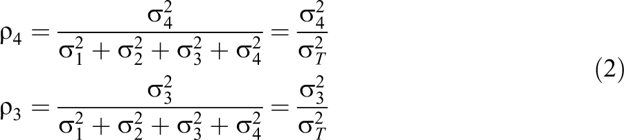
Three parameters are necessary to specify the four-level intraclass correlation structure. We define these in terms of the fraction of the total variance $σ_{T}^{2} = σ_{1}^{2} + σ_{2}^{2} + σ_{3}^{2} + σ_{4}^{2}$ explained by (unadjusted) variance across unit means at each level. Thus,

\begin{aligned} ρ_{4} = \frac{σ_{4}^{2}}{σ_{1}^{2} + σ_{2}^{2} + σ_{3}^{2} + σ_{4}^{2}} = \frac{σ_{4}^{2}}{σ_{T}^{2}} \\ ρ_{3} = \frac{σ_{3}^{2}}{σ_{1}^{2} + σ_{2}^{2} + σ_{3}^{2} + σ_{4}^{2}} = \frac{σ_{3}^{2}}{σ_{T}^{2}} \end{aligned}

and

\begin{aligned} ρ_{2} = \frac{σ_{2}^{2}}{σ_{1}^{2} + σ_{2}^{2} + σ_{3}^{2} + σ_{4}^{2}} = \frac{σ_{2}^{2}}{σ_{T}^{2}} . \end{aligned}

There is no ρ₁, but the complement of ρ₂, ρ₃, and ρ₄; namely, $\overset{ˉ}{ρ} = 1 - ρ_{2} - ρ_{3} - ρ_{4}$ is analogous to it. In three-level models, only two intraclass correlations ρ₂ and ρ₃ are necessary to specify the intraclass correlation structure, which could be defined by assuming $σ_{4}^{2} = 0$ . In two-level models, only one intraclass correlation ρ₂ is necessary to specify the intraclass correlation structure, which could be defined by assuming $σ_{3}^{2} = σ_{4}^{2} = 0$ .

Optimal Allocation in Hierarchical Designs

The goal of optimal allocation is to choose the number of units at each level in order to achieve the most sensitive design (the design with the smallest variance of the estimated treatment effect) for a fixed cost. Suppose that the total cost is a linear function of the number of units at each level. Let the cost per Level 1 unit be c ₁, the cost per Level 2 unit be c ₂, the cost per Level 3 unit be c ₃, and the cost per Level 4 unit be c ₄. Then the total cost C in a design with 2m Level 4 units, 2mr Level 3 units, 2mrp Level 2 units, and 2mrpn Level 1 units would be as follows:

C = 2 m r p n c_{1} + 2 m r p c_{2} + 2 m r c_{3} + 2 m c_{4} .

Solving Equation 3 for m yields

m = \frac{C}{2 r p n c_{1} + 2 r p c_{2} + 2 r c_{3} + 2 c_{4}} .

The variance of the treatment effect estimate is given by

\frac{({\overset{ˉ}{P}}_{1}^{2} \overset{ˉ}{ρ} + r p n {\overset{ˉ}{P}}_{4}^{2} ρ_{4} + p n {\overset{ˉ}{P}}_{3}^{2} ρ_{3} + n {\overset{ˉ}{P}}_{2}^{2} ρ_{2}) σ_{T}^{2}}{m r p n} .

Inserting Equation 4 for m into Equation 5, noting that the total cost C, the ρ _i , and the ${\overset{ˉ}{P}}_{i}^{2}$ are constants, and minimizing yields the unconstrained optimal number n _O of Level 1 units per Level 2 unit, the optimal number p _O of Level 2 units per Level 3 unit, and the optimal number r _O of Level 3 units per Level 4 unit. Setting r = 1 and c₃ = 0 in Equation 4 before inserting in Equation 5 and minimizing leads to optimal allocations in three-level hierarchical designs and also setting p = 1 and c ₂ = 0 in Equation 4 before inserting in Equation 5 and minimizing leads to optimal allocations in two-level hierarchical designs.

Expressions for optimal allocations in two-, three-, and four-level hierarchical designs are given in the left panel of Table 1. The table reveals that the optimal allocations depend on the cost ratios and the intraclass correlation ratios for adjacent levels, but in an inverse relation (understanding that $\overset{ˉ}{ρ}$ is analogous to ρ₁). For example, the optimal allocation for Level 2 in a four-level design depends on the product of c ₃/c ₂ and ρ₂/ρ₃.

Table 1

Unconstrained Optimal Allocations in Two-, Three-, and Four-Level Designs

Hierarchical Design	Randomized Block Design
Two-level designs
$n_{O} = \sqrt{(\frac{c_{2}}{c_{1}}) (\frac{{\overset{ˉ}{P}}_{1}^{2} (1 - ρ_{2})}{{\overset{ˉ}{P}}_{2}^{2} ρ_{2}})}$	$n_{O} = \sqrt{(\frac{c_{2}}{2 c_{1}}) (\frac{{\overset{ˉ}{P}}_{1}^{2} (1 - ρ_{2})}{n {\overset{ˉ}{Q}}_{2}^{2} ω ρ_{2}})}$
Three-level designs
	Assigning subclusters to treatments
$n_{O} = \sqrt{(\frac{c_{2}}{c_{1}}) (\frac{{\overset{ˉ}{P}}_{1}^{2} (1 - ρ_{2} - ρ_{3})}{{\overset{ˉ}{P}}_{2}^{2} ρ_{2}})}$	$n_{O} = \sqrt{(\frac{c_{2}}{c_{1}}) (\frac{{\overset{ˉ}{P}}_{1}^{2} (1 - ρ_{2} - ρ_{3})}{{\overset{ˉ}{P}}_{2}^{2} ρ_{2}})}$
$p_{O} = \sqrt{(\frac{c_{3}}{c_{2}}) (\frac{{\overset{ˉ}{P}}_{2}^{2} ρ_{2}}{{\overset{ˉ}{P}}_{3}^{2} ρ_{3}})}$	$p_{O} = \sqrt{(\frac{c_{3}}{2 c_{2}}) (\frac{{\overset{ˉ}{P}}_{2}^{2} ρ_{2}}{{\overset{ˉ}{Q}}_{3}^{2} ω_{3} ρ_{3}})}$
Four-level designs
	Assigning subclusters to treatments
$n_{O} = \sqrt{(\frac{c_{2}}{c_{1}}) (\frac{{\overset{ˉ}{P}}_{1}^{2} (1 - ρ_{2} - ρ_{3} - ρ_{4})}{{\overset{ˉ}{P}}_{2}^{2} ρ_{2}})}$	$n_{O} = \sqrt{(\frac{c_{2}}{c_{1}}) (\frac{{\overset{ˉ}{P}}_{1}^{2} (1 - ρ_{2} - ρ_{3} - ρ_{4})}{{\overset{ˉ}{P}}_{2}^{2} ρ_{2}})}$
$p_{O} = \sqrt{(\frac{c_{3}}{c_{2}}) (\frac{{\overset{ˉ}{P}}_{2}^{2} ρ_{2}}{{\overset{ˉ}{P}}_{3}^{2} ρ_{3}})}$	$p_{O} = \sqrt{(\frac{c_{3}}{c_{2}}) (\frac{{\overset{ˉ}{P}}_{2}^{2} ρ_{2}}{{\overset{ˉ}{P}}_{3}^{2} ρ_{3}})}$
$r_{O} = \sqrt{(\frac{c_{4}}{c_{3}}) (\frac{{\overset{ˉ}{P}}_{3}^{2} ρ_{3}}{{\overset{ˉ}{P}}_{4}^{2} ρ_{4}})}$	$r_{O} = \sqrt{(\frac{c_{4}}{2 c_{3}}) (\frac{{\overset{ˉ}{P}}_{3}^{2} ρ_{3}}{{\overset{ˉ}{Q}}_{4}^{2} ω_{4} ρ_{4}})}$

Constrained Optimal Allocation in Hierarchical Designs

Optimal design methods provide useful guidance in designing multilevel experiments, but should rarely be the only consideration in choosing a research design. Practical considerations are also important. For example, one might expect attrition of units at various levels, so selecting a very small number of replications at a level may be unwise because loss of a few units to attrition might lead to losses of entire higher level units. For example, one classroom per school might be optimal in terms of efficiency, but loss of that one classroom to attrition could lead to loss of the entire school, which could have a substantial effect on precision or statistical power. Alternatively, the experiment might have secondary goals in addition to estimation of the treatment effect. For example, if the treatment was believed to be difficult to implement, a secondary goal might be to estimate the between-classroom variance among the treated versus the untreated units. In that case, it might be determined that at least two (or more) classrooms per school would be required.

It often occurs that we wish to find the most efficient design subject to fixed constraints on the number of units at one or more levels. In the motivating example, the funding agency dictated a requirement that school districts would be assigned to treatments and that there would be exactly p = 2 schools per district. In this case, we might wish to find the most efficient design, given a decision to have at least two schools per district. If unconstrained optimal design dictates that fewer than two schools per district would be optimal, the problem becomes that of finding the optimal design under the constraint that there are exactly two schools per district. Similarly, the unconstrained optimal design might dictate that fewer than 10 students per classroom would be optimal, but we may wish to avoid pulling individual students out of classrooms for testing, so that we will test the entire group of 22 students per classroom. In this case, the problem would become that of finding the optimal number of classrooms, given the constraint that there are 22 students per classroom.

Constrained optimal allocations are obtained by inserting the Equation 4 for m into Equation 5 and minimizing, but now assuming that one or more of r, p, or n are fixed in addition to the total cost C, the ρ _i , and the ${\overset{ˉ}{P}}_{i}^{2}$ . Constrained optimal allocations in three-level hierarchical designs are obtained by setting r = 1 and c ₃ = 0 in Equation 4 for m and inserting the result in Equation 5 and minimizing, assuming that one of p or n is fixed in addition to the total cost C, the ρ _i , and the ${\overset{ˉ}{P}}_{i}^{2}$ .

Expressions for the constrained optimal allocations in three- and four-level hierarchical designs are given in the left-hand panel of Table 2. The top portion of the table gives the constrained optimal allocations in three-level designs with one fixed allocation. The middle portion of the table gives constrained optimal allocations in four-level hierarchical designs with one fixed allocation, and the bottom portion of the table gives constrained optimal allocations in four-level hierarchical designs with two fixed allocations. It is perhaps not obvious from the formulas, but the constrained optimal allocations are consistent with the unconstrained optimal allocations in the sense that if the allocation at any level is constrained to be the unconstrained optimal allocation, the constrained allocation of the remaining levels is equal to the unconstrained optimal allocation. For example, if the unconstrained optimal allocations at Level 1 and 2 of a three-level design are n _O = 9.7 and p _O = 6.5, then the constrained optimal allocations with p constrained to be 6.5 will be n _CO = 9.7, and the constrained optimal allocations with n constrained to be 9.7 will be p _CO = 6.5. This consistency property is illustrated in Table 3 by the constrained optimal allocations when the constraint equals the unconstrained optimal allocation (boldface type).

Table 2

Constrained Optimal Allocations in Three- and Four-Level Designs

Hierarchical Design	Randomized Block Design
Three-level designs
Fixed p optimizing n
$n_{C O} = \sqrt{(\frac{p c_{2} + c_{3}}{p c_{1}}) (\frac{{\overset{ˉ}{P}}_{1}^{2} (1 - ρ_{2} - ρ_{3})}{{\overset{ˉ}{P}}_{2}^{2} ρ_{2} + p {\overset{ˉ}{P}}_{3}^{2} ρ_{3}})}$	$n_{C O} = \sqrt{(\frac{2 p c_{2} + c_{3}}{2 p c_{1}}) (\frac{{\overset{ˉ}{P}}_{1}^{2} (1 - ρ_{2} - ρ_{3})}{{\overset{ˉ}{P}}_{2}^{2} ρ_{2} + p {\overset{ˉ}{Q}}_{3}^{2} ω_{3} ρ_{3}})}$
Fixed n optimizing p
$p_{C O} = \sqrt{(\frac{c_{3}}{n c_{1} + c_{2}}) (\frac{{\overset{ˉ}{P}}_{1}^{2} (1 - ρ_{2} - ρ_{3}) + n {\overset{ˉ}{P}}_{2}^{2} ρ_{2}}{n {\overset{ˉ}{P}}_{3}^{2} ρ_{3}})}$	$p_{C O} = \sqrt{(\frac{c_{3}}{2 n c_{1} + 2 c_{2}}) (\frac{{\overset{ˉ}{P}}_{1}^{2} (1 - ρ_{2} - ρ_{3}) + n {\overset{ˉ}{P}}_{2}^{2} ρ_{2}}{{\overset{ˉ}{Q}}_{3}^{2} ω_{3} ρ_{3}})}$
Four-level designs
Fixed r optimizing p and n
$p_{C O} = \sqrt{(\frac{r c_{3} + c_{4}}{r c_{2}}) (\frac{{\overset{ˉ}{P}}_{2}^{2} ρ_{2}}{{\overset{ˉ}{P}}_{3}^{2} ρ_{3} + r {\overset{ˉ}{P}}_{4}^{2} ρ_{4}})}$	$p_{C O} = \sqrt{(\frac{2 r c_{3} + c_{4}}{2 r c_{2}}) (\frac{{\overset{ˉ}{P}}_{2}^{2} ρ_{2}}{{\overset{ˉ}{P}}_{3}^{2} ρ_{3} + r {\overset{ˉ}{Q}}_{4}^{2} ω_{4} ρ_{4}})}$
$n_{O} = \sqrt{(\frac{c_{2}}{c_{1}}) (\frac{{\overset{ˉ}{P}}_{1}^{2} \overset{ˉ}{ρ}}{{\overset{ˉ}{P}}_{2}^{2} ρ_{2}})}$	$n_{C O} = \sqrt{(\frac{c_{2}}{c_{1}}) (\frac{{\overset{ˉ}{P}}_{1}^{2} \overset{ˉ}{ρ}}{{\overset{ˉ}{P}}_{2}^{2} ρ_{2}})}$
Fixed p optimizing r and n
$r_{C O} = \sqrt{(\frac{c_{4}}{p c_{2} + c_{3}}) (\frac{{\overset{ˉ}{P}}_{2}^{2} ρ_{2} + p {\overset{ˉ}{P}}_{3}^{2} ρ_{3}}{p {\overset{ˉ}{P}}_{4}^{2} ρ_{4}})}$	$r_{O} = \sqrt{(\frac{c_{4}}{2 p c_{2} + 2 c_{3}}) (\frac{{\overset{ˉ}{P}}_{2}^{2} ρ_{2} + p {\overset{ˉ}{P}}_{3}^{2} ρ_{3}}{p {\overset{ˉ}{Q}}_{4}^{2} ω_{4} ρ_{4}})}$
$n_{C O} = \sqrt{(\frac{p c_{2} + c_{3}}{p c_{1}}) (\frac{{\overset{ˉ}{P}}_{1}^{2} \overset{ˉ}{ρ}}{{\overset{ˉ}{P}}_{2}^{2} ρ_{2} + p {\overset{ˉ}{P}}_{3}^{2} ρ_{3}})}$	$n_{C O} = \sqrt{(\frac{p c_{2} + c_{3}}{p c_{1}}) (\frac{{\overset{ˉ}{P}}_{1}^{2} \overset{ˉ}{ρ}}{{\overset{ˉ}{P}}_{2}^{2} ρ_{2} + p {\overset{ˉ}{P}}_{3}^{2} ρ_{3}})}$
Fixed n optimizing r and p
$r_{C O} = \sqrt{(\frac{c_{4}}{c_{3}}) (\frac{{\overset{ˉ}{P}}_{3}^{2} ρ_{3}}{{\overset{ˉ}{P}}_{4}^{2} ρ_{4}})}$	$r_{C O} = \sqrt{(\frac{c_{4}}{2 c_{3}}) (\frac{{\overset{ˉ}{P}}_{3}^{2} ρ_{3}}{{\overset{ˉ}{Q}}_{4}^{2} ω_{4} ρ_{4}})}$
$p_{C O} = \sqrt{(\frac{c_{3}}{n c_{1} + c_{2}}) (\frac{{\overset{ˉ}{P}}_{1}^{2} \overset{ˉ}{ρ} + n {\overset{ˉ}{P}}_{2}^{2} ρ_{2}}{n {\overset{ˉ}{P}}_{3}^{2} ρ_{3}})}$	$p_{C O} = \sqrt{(\frac{c_{3}}{n c_{1} + c_{2}}) (\frac{{\overset{ˉ}{P}}_{1}^{2} \overset{ˉ}{ρ} + n {\overset{ˉ}{P}}_{2}^{2} ρ_{2}}{n {\overset{ˉ}{P}}_{3}^{2} ρ_{3}})}$
Fixed r and p optimizing n
$n_{C O} = \sqrt{(\frac{r p c_{2} + r c_{3} + c_{4}}{r p c_{1}}) (\frac{{\overset{ˉ}{P}}_{1}^{2} \overset{ˉ}{ρ}}{{\overset{ˉ}{P}}_{2}^{2} ρ_{2} + p {\overset{ˉ}{P}}_{3}^{2} ρ_{3} + r p {\overset{ˉ}{P}}_{4}^{2} ρ_{4}})}$	$n_{C O} = \sqrt{(\frac{2 r p c_{2} + 2 r c_{3} + c_{4}}{2 r p c_{1}}) (\frac{{\overset{ˉ}{P}}_{1}^{2} \overset{ˉ}{ρ}}{{\overset{ˉ}{P}}_{2}^{2} ρ_{2} + p {\overset{ˉ}{P}}_{3}^{2} ρ_{3} + r p {\overset{ˉ}{Q}}_{4}^{2} ω_{4} ρ_{4}})}$
Fixed p and n optimizing r
$r_{C O} = \sqrt{(\frac{c_{4}}{p n c_{1} + p c_{2} + c_{3}}) (\frac{{\overset{ˉ}{P}}_{1}^{2} \overset{ˉ}{ρ} + n {\overset{ˉ}{P}}_{2}^{2} ρ_{2} + p n {\overset{ˉ}{P}}_{3}^{2} ρ_{3}}{p n {\overset{ˉ}{P}}_{4}^{2} ρ_{4}})}$	$r_{C O} = \sqrt{(\frac{c_{4}}{p n c_{1} + p c_{2} + c_{3}}) (\frac{{\overset{ˉ}{P}}_{1}^{2} \overset{ˉ}{ρ} + n {\overset{ˉ}{P}}_{2}^{2} ρ_{2} + p n {\overset{ˉ}{P}}_{3}^{2} ρ_{3}}{2 p n {\overset{ˉ}{Q}}_{4}^{2} ω_{4} ρ_{4}})}$
Fixed r and n optimizing p
$p_{C O} = \sqrt{(\frac{r c_{3} + c_{4}}{r n c_{1} + r c_{2}}) (\frac{{\overset{ˉ}{P}}_{1}^{2} \overset{ˉ}{ρ} + n {\overset{ˉ}{P}}_{2}^{2} ρ_{2}}{n {\overset{ˉ}{P}}_{3}^{2} ρ_{3} + r n {\overset{ˉ}{P}}_{4}^{2} ρ_{4}})}$	$p_{C O} = \sqrt{(\frac{2 r c_{3} + c_{4}}{2 r n c_{1} + 2 r c_{2}}) (\frac{{\overset{ˉ}{P}}_{1}^{2} \overset{ˉ}{ρ} + n {\overset{ˉ}{P}}_{2}^{2} ρ_{2}}{n {\overset{ˉ}{P}}_{3}^{2} ρ_{3} + r n {\overset{ˉ}{Q}}_{4}^{2} ω_{4} ρ_{4}})}$

Note. Here $\overset{ˉ}{ρ} = 1 - ρ_{2} - ρ_{3} - ρ_{4}$ .

Table 3

Unconstrained and Constrained Optimal Allocations for Three-Level Hierarchical Designs

		Unconstrained		Constrained
ρ₂	ρ₃	p _O	n _O	p	n _CO	n	p _CO
Cost ratios c ₃ = 5c ₂, c ₂ = 10c ₁
0.19	0.01	9.7	6.5	1	15.5	1	21.2
0.19	0.01	9.7	6.5	2	11.5	2	15.7
0.19	0.01	9.7	6.5	3	9.8	4	11.8
0.19	0.01	9.7	6.5	4	8.8	6	10.1
0.19	0.01	9.7	6.5	5	8.2	6.5	9.7
0.19	0.01	9.7	6.5	6	7.7	8	9.0
0.19	0.01	9.7	6.5	8	6.9	10	8.2
0.19	0.01	9.7	6.5	9.7	6.5	15	7.0
0.19	0.01	9.7	6.5	15	5.6	20	6.2
0.19	0.01	9.7	6.5	20	5.1	50	4.1
0.10	0.10	2.2	8.9	1	15.5	1	6.4
0.10	0.10	2.2	8.9	2	9.7	2	4.6
0.10	0.10	2.2	8.9	2.2	8.9	4	3.3
0.10	0.10	2.2	8.9	3	7.3	6	2.7
0.10	0.10	2.2	8.9	4	6.0	8	2.4
0.10	0.10	2.2	8.9	6	4.6	8.9	2.2
0.10	0.10	2.2	8.9	8	3.8	15	1.8
0.10	0.10	2.2	8.9	10	3.3	20	1.5
0.10	0.10	2.2	8.9	20	2.2	50	1.0
0.01	0.19	0.5	28.3	0.5	28.3	5	1.7
0.01	0.19	0.5	28.3	1	15.5	10	1.1
0.01	0.19	0.5	28.3	2	8.5	15	0.8
0.01	0.19	0.5	28.3	3	6.1	20	0.7
0.01	0.19	0.5	28.3	5	4.1	25	0.6
0.01	0.19	0.5	28.3	10	2.5	28.3	0.5
0.01	0.19	0.5	28.3	20	1.6	50	0.3
Cost ratios c ₃ = 2c ₂, c ₂ = 2c ₁
0.19	0.01	4.4	2.9	1	4.0	1	8.1
0.19	0.01	4.4	2.9	2	3.4	2	5.4
0.19	0.01	4.4	2.9	3	3.1	2.9	4.4
0.19	0.01	4.4	2.9	4	2.9	4	3.6
0.19	0.01	4.4	2.9	4.4	2.9	6	2.8
0.19	0.01	4.4	2.9	6	2.7	10	2.1
0.19	0.01	4.4	2.9	8	2.6	15	1.7
0.19	0.01	4.4	2.9	10	2.5	20	1.4
0.19	0.01	4.4	2.9	20	2.1	25	1.3
0.19	0.01	4.4	2.9	30	1.8	30	1.2
0.19	0.01	4.4	2.9	40	1.7	40	1.0
0.10	0.10	1.0	4.0	1.0	4.0	1	2.4
0.10	0.10	1.0	4.0	2	2.8	2	1.6
0.10	0.10	1.0	4.0	3	2.3	3	1.2
0.10	0.10	1.0	4.0	4	2.0	4.0	1.0
0.01	0.19	0.2	12.6	0.2	12.6	1	1.7
0.01	0.19	0.2	12.6	1	4.0	2	1.0
0.01	0.19	0.2	12.6	2	2.5	4	0.6
0.01	0.19	0.2	12.6	3	1.9	6	0.4
0.01	0.19	0.2	12.6	4	1.6	8	0.3
0.01	0.19	0.2	12.6	10	1.0	12.6	0.2

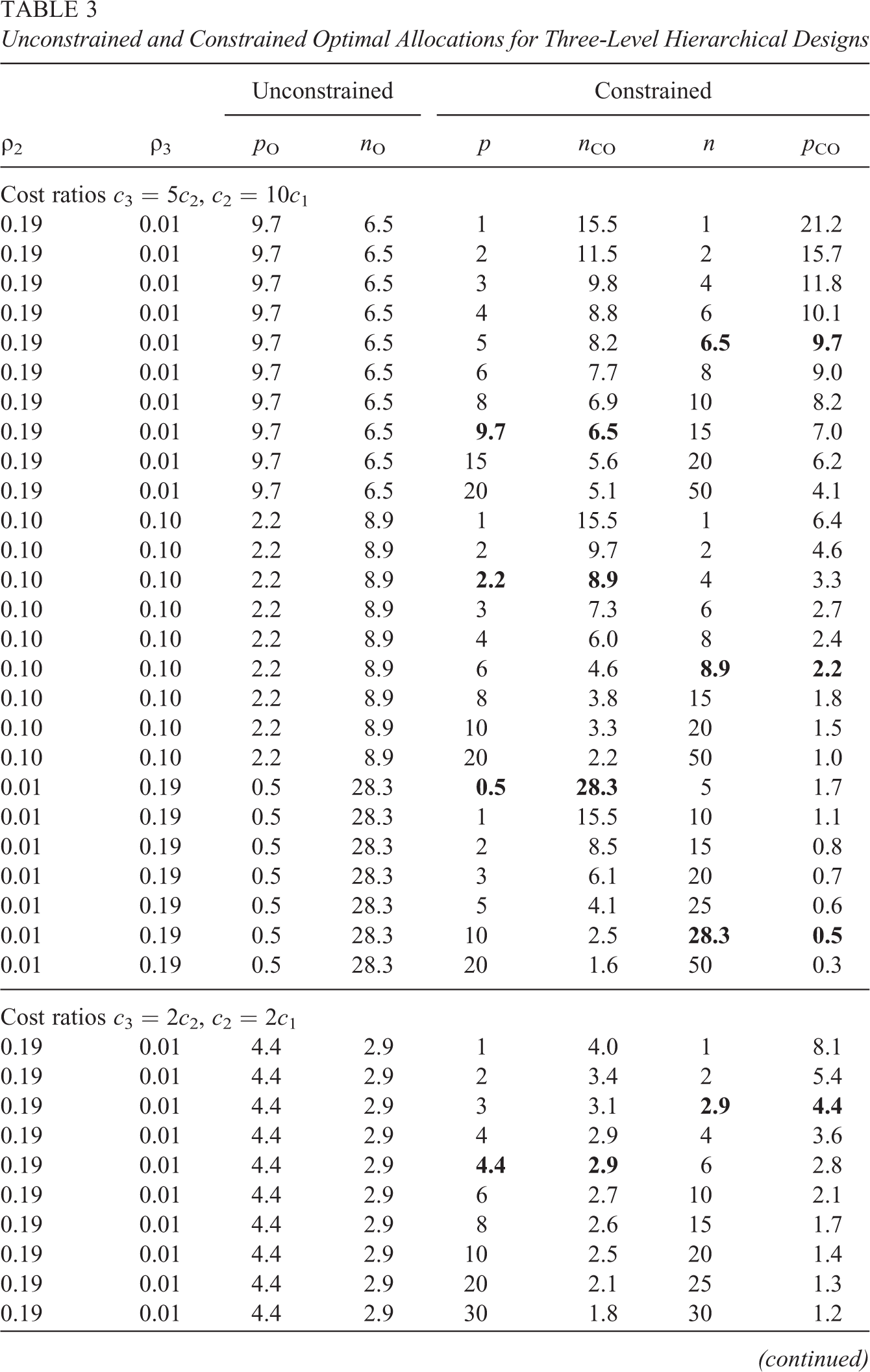
In three-level designs, the constrained optimal allocations (optimal n for fixed p or optimal p for fixed n) are both different from the corresponding unconstrained optimal allocations given in Table 1. Taking the derivative of n _CO as function of the constraint p, we see that n _CO is decreasing function of p and that n _CO = n _O (the unconstrained optimal allocation at Level 1) exactly when p = p _O (the unconstrained optimal allocation at Level 2). Therefore, when p < p _O, n _CO > n _O, and when p > p _O, n _CO < n _O. Taking the derivative of p _CO as function of the constraint n, we see that p _CO is decreasing function of n and that p _CO = p _O (the unconstrained optimal allocation at Level 2) exactly when n = n _O (the unconstrained optimal allocation at Level 1). Therefore, when n < n _O, p _CO > p _O, and when n > n _O, p _CO < p _O. That is, constraining the allocation at a level to be smaller than the unconstrained optimal allocation at that level leads to constrained optimal allocation at adjacent levels that are larger than optimal allocation. Similarly, constraining the allocation at a level to be larger than the unconstrained optimal allocation leads to constrained optimal allocation at adjacent levels that are smaller than their unconstrained optimal allocations.

The fact that n _CO is a decreasing function of p and that p _CO is a decreasing function of n is illustrated in Table 3 for three intraclass correlation patterns and two different cost structures. The top half of the table uses a high cost ratio structure similar to that in the motivating example, while the bottom half of the table uses a low cost ratio structure similar to the low cost ratio investigated by Raudenbush (1997). For each cost structure, three different sets of intraclass correlation structures are examined, one where ρ₂ is considerably bigger than ρ₃ (as in our motivating example), one where they are approximately equal (a pattern that is prevalent in district and school-level academic achievement in some U.S. states), and one where ρ₂ is considerably smaller than ρ₃ (a pattern that occurs, for example, with respect to school- and classroom-level academic achievement in some U.S. school districts).

In four-level hierarchical designs, Table 2 reveals that constraining the allocation at a level only has an impact on the immediately adjacent levels. That is, constraining the allocation at Level 3 has an impact on the constrained optimal allocation at Level 2 but not at Level 1, so that the constrained optimal allocation at Level 1 is the same as the unconstrained optimal allocation. Similarly, constraining the allocation at Level 1 has an impact on the constrained optimal allocation at Level 2, but not at Level 3, so that the constrained optimal allocation at Level 3 is the same as the unconstrained optimal allocation. However, constraining the allocation at Level 2 has an impact on the constrained optimal allocation at both Levels 1 and 3. As in the case of three-level constrained optimal allocations, the constrained optimal allocations that are affected by the constraint are decreasing functions of the constraint and the constrained optimal allocations equal the constrained optimal allocations only when the value of the constraint is exactly equal to the unconstrained optimal allocation for that level.

Randomized Block Designs

In this section, we describe the models underlying the results for randomized block designs presented in this article. We first describe the four-level model and then show how these can be simplified to three-level and two-level situations.

Model and Notation

Suppose that there are m clusters (Level 4 units) and that r of the subclusters (Level 3 units) in each cluster are assigned to each treatment. Suppose that each of these subclusters has p sub-subclusters (Level 2 units), with n individuals each. Let Y_ijkl be the lth observation in the kth sub-subcluster in jth subcluster of the ith cluster. Suppose that there is also a covariate W at Level 4, a covariate Z at Level 3, a covariate U at Level 2, and a covariate X at Level 1. Let Y_ijkl be the lth observation in kth sub-subcluster of the jth subcluster of the ith cluster. Thus, model is given by

\begin{aligned} Y_{i j k l} & = β_{0} + β_{1} T_{i j} + T_{i j} ζ_{1 i} + β_{2} W_{i} + γ U_{i j} + δ Z_{i j k} + π X_{i j k l} + ζ_{0 i} + η_{i j} + ξ_{i j k} + ∊_{i j k l}, \\ i & = 1, \dots, m; j = 1, \dots, 2 r; k = 1, \dots, p; l = 1, \dots, n . \end{aligned}

The fixed effects are the grand mean β₀, the covariate adjusted treatment effect β₁, the effect of the Level 4 covariate β₂, the effect of the Level 3 covariate γ, the effect of the Level 2 covariate δ, and the effect of the Level 1 covariate π. There are two kinds of random effects at Level 4: one associated with variation of the mean of Level 4 units (the ζ_0i) and one associated with the variation of the treatment effects across Level 4 units (the ζ_1i), which are assumed to be independently normally distributed with zero means and variances $σ_{A 4}^{2}$ and $τ_{A 4}^{2}$ , respectively. In addition, there are Level 3 (the η _ij ), Level 2 (the ξ _ijk ), and Level 1 (the ∊ _ijkl ) random effects, which are assumed to be independently normally distributed with zero means and variances $σ_{A 3}^{2}, σ_{A 2}^{2}, a n d σ_{A 1}^{2}$ , respectively. Here the A in the subscript of the residual variances refers to the fact that the model includes covariates, so that the variances are adjusted for the covariates; the variances in a model without covariates would be denoted by $σ_{4}^{2}, τ_{4}^{2}, σ_{3}^{2}, σ_{2}^{2}, a n d σ_{1}^{2}$ , respectively. The covariate outcome correlations are defined in terms of the adjusted and unadjusted variances as $P_{1}^{2} = 1 - {\overset{ˉ}{P}}_{1}^{2} = 1 - σ_{A 1}^{2} / σ_{1}^{2}$ , $P_{2}^{2} = 1 - {\overset{ˉ}{P}}_{2}^{2} = 1 - σ_{A 2}^{2} / σ_{2}^{2}$ , $P_{3}^{2} = 1 - {\overset{ˉ}{P}}_{3}^{2} = 1 - σ_{A 3}^{2} / σ_{3}^{2}$ , $P_{4}^{2} = 1 - {\overset{ˉ}{P}}_{4}^{2} = 1 - σ_{A 4}^{2} / σ_{4}^{2}$ , and $Q_{4}^{2} = 1 - {\overset{ˉ}{Q}}_{4}^{2} = τ_{A 4}^{2} / τ_{4}^{2}$ . Here the notation $\overset{ˉ}{P}$ is used to denote the complement of P; namely, $\overset{ˉ}{P} = 1 - P$ . The notation Q (instead of P) for the variance explained at Level 4 is used to emphasize that it refers to variance explained in the treatment effect, not variance in the unit means, as at other levels.

This model reduces to a three-level model if Level 2 is omitted, so that p = 1, $σ_{A 2}^{2} = 0$ , and the δZ_ijk and ξ _ijk terms drop out. It is sensible in this case to rename the highest two levels as Levels 3 and 2. The model reduces to a two-level model if, in addition, Level 1 is omitted, so that n = 1, $σ_{A 1}^{2} = 0,$ and the πX_ijkl and ∊ _ijkl terms drop out. It is sensible in this case to rename the highest level as Level 2 and the remaining level as Level 1.

The intraclass correlations ρ₂, ρ₃, and ρ₄, and the heterogeneity parameter ω₄ are defined in terms of the unadjusted variances as in the model with no covariates. The covariate outcome correlations are defined in terms of the adjusted ( $σ_{A i}^{2}$ and $τ_{A 4}^{2}$ ) and unadjusted ( $σ_{i}^{2}$ and $τ_{4}^{2}$ ) variances as ${\overset{ˉ}{P}}_{1}^{2} = 1 - P_{1}^{2} = 1 - σ_{A 1}^{2} / σ_{1}^{2}$ , ${\overset{ˉ}{P}}_{2}^{2} = 1 - P_{2}^{2} = 1 - σ_{A 2}^{2} / σ_{2}^{2}$ , ${\overset{ˉ}{P}}_{3}^{2} = 1 - P_{3}^{2} = 1 - σ_{A 3}^{2} / σ_{3}^{2}$ , and ${\overset{ˉ}{Q}}_{4}^{2} = 1 - Q_{4}^{2} = 1 - τ_{A 4}^{2} / τ_{4}^{2}$ .

Intraclass Correlations and Heterogeneity Parameters

Three parameters are necessary to specify the four-level intraclass correlation structure, and the intraclass correlations ρ₂, ρ₃, and ρ₄ (and $\overset{ˉ}{ρ} = 1 - ρ_{2} - <$ ) are defined in exactly the same way as in Equation 2 for the hierarchical design. However, in randomized block designs, the variance of the treatment effect also depends on an additional parameter describing the variance of the treatment effects across clusters (blocks or Level 4 units). There are alternative ways to represent this parameter, but a scale-free representation is the ratio of the variance of the treatment effects across Level 4 units ( $τ_{4}^{2}$ ) to the variance of the means of Level 4 units ( $σ_{4}^{2}$ ); that is, $ω_{4} = τ_{4}^{2} / σ_{4}^{2}$ .

Optimal Allocation in Randomized Block Designs

As in the case of hierarchical designs, the goal of optimal allocation is to choose the number of units at each level in order to achieve the most sensitive design (the design with the smallest variance of the estimated treatment effect) for a fixed cost. Suppose that the total cost is a linear function of the number of units at each level. Let the cost per Level 1 unit be c ₁, the cost per Level 2 unit be c ₂, the cost per Level 3 unit be c ₃, and the cost per Level 4 unit be c ₄. Then the total cost C in a design with m Level 4 units, 2mr Level 3 units, 2mrp Level 2 units, and 2mrpn Level 1 units would be

C = 2 m r p n c_{1} + 2 m r p c_{2} + 2 m r c_{3} + m c_{4} .

Solving Equation 7 for m yields

m = \frac{C}{2 r p n c_{1} + 2 r p c_{2} + 2 r c_{3} + c_{4}} .

The variance of the treatment effect estimate is given by

\frac{(2 {\overset{ˉ}{P}}_{1}^{2} \overset{ˉ}{ρ} + r p n {\overset{ˉ}{Q}}_{4}^{2} ω_{4} ρ_{4} + 2 p n {\overset{ˉ}{P}}_{3}^{2} ρ_{3} + 2 n {\overset{ˉ}{P}}_{2}^{2} ρ_{2}) σ_{T}^{2}}{m r p n} .

Inserting the Equation 8 for m into Equation 9, noting that the total cost C, the ρ _i , the ${\overset{ˉ}{P}}_{i}^{2}$ , and ${\overset{ˉ}{Q}}_{4}^{2} ω_{4}$ are constants, and minimizing yields the unconstrained optimal number n _O of Level 1 units per Level 2 unit, the optimal number p _O of Level 2 units per Level 3 unit, and the optimal number r _O of Level 3 units per treatment group in each Level 4 unit. Setting p = 1 and c ₂ = 0 in Equation 8 before inserting in Equation 9 with ρ₂ = 0 and minimizing leads to optimal allocations in three-level randomized block designs assigning Level 2 units to treatments and also setting n = 1 and c ₁ = 0 in Equation 8 before inserting in Equation 9, recognizing that $σ_{1}^{2} = 0$ implies $\overset{ˉ}{ρ} = 0$ and that minimizing leads to optimal allocations in two-level randomized block designs.

Expressions for optimal allocations in two-, three-, and four-level hierarchical designs are given in the right-hand panel of Table 1. The table reveals that the optimal allocations depend on the cost ratios and the intraclass correlation ratios for adjacent levels, but in an inverse relation (understanding that $\overset{ˉ}{ρ}$ is analogous to ρ₁). For example, the optimal allocation for Level 2 in a four-level design depends on the product of c ₃/c ₂ and ρ₂/ρ₃.

Constrained Optimal Allocation in Randomized Block Designs

Optimal design methods provide useful guidance in designing randomized block experiments, but practical considerations are also important. As in the case of experiments with hierarchical designs, we sometimes wish to find the most efficient design subject to fixed constraints on the number of units at one or more levels. We discuss later an example of a four-level randomized block design carried out by Glazerman et al. (2010) and how much the cost could be reduced by optimal allocation or by constrained optimal allocation.

Constrained optimal allocations are obtained by inserting the Equation 8 for m into Equation 9 and minimizing, but now assuming that one or more of r, p, or n are fixed in addition to the total cost C, the ρ _i , the ${\overset{ˉ}{P}}_{i}^{2}$ , and ${\overset{ˉ}{Q}}_{4}^{2} ω_{4}$ . Constrained optimal allocations in three-level hierarchical designs are obtained by setting p = 1 and c ₂ = 0 in the Equation 8 for m and inserting the result (with ρ₂ = 0) in Equation 9 and minimizing, assuming that one of p or n is fixed in addition to the total cost C, the ρ _i , the ${\overset{ˉ}{P}}_{i}^{2}$ , and ${\overset{ˉ}{Q}}_{4}^{2} ω_{4}$ .

Expressions for the constrained optimal allocations in three- and four-level hierarchical designs are given in the right-hand panel of Table 2. The top portion of the table gives the constrained optimal allocations in three-level designs with one fixed allocation. The middle portion of the table gives constrained optimal allocations in four-level randomized block designs with one fixed allocation, and the bottom portion of the table gives constrained optimal allocations in four-level randomized block designs with two fixed allocations.

The basic pattern of the constrained optimal allocations in randomized block designs is similar to that is hierarchical designs. The major difference is that ${\overset{ˉ}{Q}}_{4}^{2} ω_{4} ρ_{4}$ plays the role that corresponds to the role ${\overset{ˉ}{P}}_{4}^{2} ρ_{4}$ plays in hierarchical designs. Table 4 provides examples of optimal and constrained optimal allocations for three intraclass correlation patterns, two different cost structures, and two different values of the treatment effect heterogeneity parameter ω in three-level randomized block designs. The boldface values illustrate that the constrained optimal allocations are consistent with the unconstrained optimal allocations in the sense that if the allocation at any level is constrained to be the unconstrained optimal allocation, constrained allocation of the remaining levels is equal to the unconstrained optimal allocation.

Table 4

Unconstrained and Constrained Optimal Allocations for Three-Level Randomized Block Experiments

		ω = 0.1						ω = 0.5
		Unconstrained		Constrained		Constrained		Unconstrained		Constrained		Constrained
ρ₂	ρ₃	p _O	n _O	p	n _CO	n	p _CO	p _O	n _O	p	n _CO	n	p _CO
Cost ratios c ₃ = 5c ₂, c ₂ = 10c ₁
0.19	0.01	21.8	6.5	2	9.7	4	26.4	9.7	6.5	2	9.5	4	11.8
0.19	0.01	21.8	6.5	5	7.8	6	22.5	9.7	6.5	4	7.9	6	10.1
0.19	0.01	21.8	6.5	10	7.1	6.5	21.8	9.7	6.5	6	7.2	6.5	9.7
0.19	0.01	21.8	6.5	15	6.7	10	18.4	9.7	6.5	8	6.8	8	9.0
0.19	0.01	21.8	6.5	20	6.5	15	15.6	9.7	6.5	9.7	6.5	10	8.2
0.19	0.01	21.8	6.5	21.8	6.5	20	13.8	9.7	6.5	15	5.9	15	7.0
0.19	0.01	21.8	6.5	25	6.4	30	11.6	9.7	6.5	20	5.6	20	6.2
0.10	0.10	5.0	8.9	2	12.2	4	7.3	2.2	8.9	1	13.7	4	3.3
0.10	0.10	5.0	8.9	3	10.6	5	6.6	2.2	8.9	2.2	8.9	6	2.7
0.10	0.10	5.0	8.9	4	9.6	8.9	5.0	2.2	8.9	3	7.7	8	2.4
0.10	0.10	5.0	8.9	5.0	8.9	10	4.7	2.2	8.9	5	5.9	8.9	2.2
0.10	0.10	5.0	8.9	6	8.4	15	3.9	2.2	8.9	10	4.1	10	2.1
0.10	0.10	5.0	8.9	10	7.1	20	3.4	2.2	8.9	15	3.3	15	1.8
0.10	0.10	5.0	8.9	20	5.5	30	2.8	2.2	8.9	20	2.9	20	1.5
0.01	0.19	1.1	28.3	1	31.1	4	4.4	0.5	28.3	0.5	28.3	4	2.0
0.01	0.19	1.1	28.3	1.1	28.3	8	2.8	0.5	28.3	1	16.3	8	1.3
0.01	0.19	1.1	28.3	2	19.4	15	1.8	0.5	28.3	2	9.5	12	1.0
0.01	0.19	1.1	28.3	4	12.3	10	2.4	0.5	28.3	3	7.1	20	0.7
0.01	0.19	1.1	28.3	6	9.6	15	1.8	0.5	28.3	5	5.0	25	0.6
0.01	0.19	1.1	28.3	10	7.1	28.3	1.1	0.5	28.3	10	3.2	28.3	0.5
0.01	0.19	1.1	28.3	20	4.8	35	1.0	0.5	28.3	20	2.2	35	0.4
Cost ratios c ₃ = 2c ₂, c ₂ = 2c ₁
0.19	0.01	13.8	2.9	2	3.5	2	17.2	6.2	2.9	2	3.5	2	7.7
0.19	0.01	13.8	2.9	5	3.1	2.9	13.8	6.2	2.9	4	3.1	2.9	6.2
0.19	0.01	13.8	2.9	10	3.0	5	10.0	6.2	2.9	6.2	2.9	4	5.1
0.19	0.01	13.8	2.9	13.8	2.9	10	6.7	6.2	2.9	10	2.7	6	4.0
0.19	0.01	13.8	2.9	15	2.9	15	5.4	6.2	2.9	15	2.5	10	3.0
0.19	0.01	13.8	2.9	20	2.8	20	4.6	6.2	2.9	20	2.4	15	2.4
0.19	0.01	13.8	2.9	30	2.7	30	3.7	6.2	2.9	30	2.2	20	2.0
0.10	0.10	3.2	4.0	2	4.5	3	3.8	1.4	4.0	1	4.6	2	2.2
0.10	0.10	3.2	4.0	3.2	4.0	4.0	3.2	1.4	4.0	1.4	4.0	3	1.7
0.10	0.10	3.2	4.0	4	3.8	6	2.4	1.4	4.0	2	3.5	4.0	1.4
0.10	0.10	3.2	4.0	10	3.0	10	1.7	1.4	4.0	4	2.6	6	1.1
0.10	0.10	3.2	4.0	20	2.4	20	1.1	1.4	4.0	10	1.7	8	0.9
0.01	0.19	0.7	12.6	0.7	12.6	4	1.9	0.3	12.6	0.3	12.6	3	1.1
0.01	0.19	0.7	12.6	1	10.5	8	1.1	0.3	12.6	1	5.5	5	0.7
0.01	0.19	0.7	12.6	2	7.1	10	0.9	0.3	12.6	2	3.5	8	0.5
0.01	0.19	0.7	12.6	3	5.6	12.6	0.7	0.3	12.6	4	2.3	10	0.4
0.01	0.19	0.7	12.6	5	4.3	15	0.6	0.3	12.6	10	1.4	12.6	0.3

As in hierarchical designs, constraining the allocation at a level only has an impact on the immediately adjacent levels. The constrained optimal allocations in nonadjacent levels are the same as the corresponding unconstrained optimal allocations. For levels that are affected by the constraint, the constrained optimal allocation is a decreasing function of the value of the constraint and the constrained optimal allocation equals the unconstrained optimal allocation only when the value of the constraint equals the unconstrained optimal allocation for the level being constrained.

Obtaining Intraclass Correlations for Optimal Design

The use of optimal allocation methods described in this article requires access to information on intraclass correlations and evidence about variance explained by covariates at various levels of the design (which we refer to as design parameters in this section). Because these design parameters are also necessary for power analysis in cluster randomized designs, there has been considerable effort to accumulate data on these parameters. For example, Bloom, Richburg-Hayes, and Black (2007) provided estimates of two-level design parameters based on data from five large urban school districts in the United States. Hedges and Hedberg (2007) provided estimates of two-level design parameters for reading and mathematics achievement in Grades Kindergarten to 12 using data from educational surveys that have U.S. national probability samples. The published data are supplemented by a web archive providing design parameters for subsets of the country by region of the country, achievement level of schools, and ethnic composition of schools. Jacob, Zhu, and Bloom (2010) extended the Bloom et al. database by providing three-level design parameters (students within classrooms within schools) estimated from five large school districts.

More recently, the development of U.S. state longitudinal data systems (currently in 46 of the 50 U.S. states) has provided a new opportunity to develop estimates of multilevel design parameters. Hedges and Hedberg (in press) have developed a new web resource that provides three- and four-level (students within classes within schools within school districts) design parameters based on state longitudinal data. The database currently includes estimates of design parameters for 11 U.S. states, but additional states are being added as data become available (http://www.ipr.northwestern.edu/research-areas/designparameters/stateva.html). Moreover, the project is providing software and training, so that states can develop the capacity to produce design parameters themselves on a regular basis and make them available to researchers as part of their data system. This research has found different patterns of school- and district-level intraclass correlations in different states. In some states (like Arkansas, Florida, and Kentucky), they find a pattern of relatively small district-level intraclass correlations (e.g., ρ₃ = 0.01–0.04) and larger school within-district intraclass correlations (e.g., ρ₂ = 0.11–0.24), while in other states (like Arizona and Massachusetts) the school- and district-level intraclass correlations are approximately equal (e.g., ρ₂ = ρ₃ = 0.11).

Published compilations of intraclass correlation data at more than two levels are rarer in substantive areas outside of education. Representative values in the health sciences were cited in Murray, Hannan, and Baker (1996), who suggested that ρ₂ + ρ₃ ≤ 0.05 was typical with ρ₂/ρ₃ ranging from about 0.25 to 4. Similarly, compilations of values of treatment effect heterogeneity parameters used in randomized block designs are rather sparse (see Weiss, Bloom, & Brock, 2013). Schochet (2008) cited values from several experiments and generally argued that the variance of treatment effects would be expected to be small in most education and social science contexts, with values of the ω parameter on the order of ω = 0.1.

Robustness to Misspecification of Intraclass Correlations

The robustness of optimal allocations to incorrect assumptions about intraclass correlations in two-level designs was studied by Korendijk et al. (2010). They did so by fixing the total cost and computing the relative efficiency of estimated treatment effects of optimal allocations computed from incorrectly versus correctly specified intraclass correlations. They argued that a relative efficiency of 90% is considered good and a relative efficiency of 80% to 90% is generally considered acceptable. For several values of intraclass correlation and cost ratios, they found that relative efficiency was at least 90% when the optimal allocation was based on an intraclass correlation between 25% and 175% of the true value.

While an extensive study of the robustness of constrained optimal allocations is beyond the scope of this article, we did conduct some limited studies of robustness of constrained optimal designs with three levels, three different intraclass correlation structures, and two different cost structures. One cost structure involved relatively low cost ratios c ₃ = 2c ₂ = 4c ₁, which is similar to the low cost ratio scenario (c ₂ = 2c ₁) examined by Korendijk et al. (2010). The second cost structure involved higher cost ratios: c ₃ = 5c ₂ = 50c ₁, which is similar to the cost ratio in our motivating example and to the high cost ratio scenario (c ₂ = 50c ₁) examined by Korendijk et al. Table 5 provides some examples of the relative efficiency of three-level hierarchical designs using constrained optimal allocation when the Level 2 allocation, p, is constrained. Table 6 provides some examples of the relative efficiency of three-level hierarchical designs using constrained optimal allocation when the Level 1 allocation, n, is constrained. It is evident from the tables (and somewhat more extensive computations not shown) that underestimation of the intraclass correlations impairs efficiency more than overestimation. However, across the situations studied, underestimating both ρ₂ and ρ₃ by 75% still yields relative efficiency of efficiency over 80%, and underestimating both ρ₂ and ρ₃ by 67% still yields relative efficiency of over 90%. While more work is needed to investigate the robustness of constrained optimal allocations to misspecification of intraclass correlations, the limited work we have done suggests that they are reasonably robust.

Table 5

Relative Efficiency of the Constrained Optimal Design Constraining p When Intraclass Correlations Are Misspecified

				Assumed Value of Intraclass Correlations
Actual Intraclass Correlations				0.25 ρ₂			1.0 ρ₂			1.75 ρ₂
ρ₂	ρ₃	p _O	p	0.25 ρ₃	1.0 ρ₃	1.75 ρ₃	0.25 ρ₃	1.0 ρ₃	1.75 ρ₃	0.25 ρ₃	1.0 ρ₃	1.75 ρ₃
Cost ratios c ₃ = 5c ₂, c ₂ = 10c ₁
0.19	0.01	9.7	2	0.89	0.93	0.95	1.00	1.00	1.00	0.98	0.98	0.97
0.19	0.01	9.7	10	0.88	0.96	0.99	1.00	1.00	1.00	0.99	0.98	0.97
0.19	0.01	9.7	20	0.88	0.98	1.00	0.99	1.00	0.99	1.00	0.99	0.97
0.10	0.10	2.2	1	0.91	0.99	1.00	0.99	1.00	0.99	1.00	0.99	0.98
0.10	0.10	2.2	2	0.90	0.99	1.00	0.97	1.00	0.99	1.00	1.00	0.98
0.10	0.10	2.2	4	0.90	1.00	0.99	0.96	1.00	0.99	0.99	1.00	0.98
0.01	0.19	0.5	1	0.91	1.00	1.00	0.92	1.00	0.98	0.94	1.00	0.98
0.01	0.19	0.5	10	0.93	1.00	1.00	0.93	1.00	0.98	0.93	1.00	0.98
Cost ratios c ₃ = 2c ₂, c ₂ = 2c ₁
0.19	0.01	6.2	2	0.86	0.90	0.93	1.00	1.00	1.00	0.97	0.97	0.96
0.19	0.01	6.2	6	0.86	0.94	0.97	1.00	1.00	1.00	0.98	0.97	0.96
0.19	0.01	6.2	15	0.86	0.97	1.00	0.99	1.00	1.00	1.00	0.98	0.96
0.10	0.10	1.4	1	0.86	0.98	1.00	0.98	1.00	0.99	1.00	0.99	0.96
0.10	0.10	1.4	5	0.87	1.00	0.99	0.93	1.00	0.98	0.97	1.00	0.97
0.01	0.19	0.3	1	0.86	1.00	0.97	0.89	1.00	0.97	0.91	1.00	0.96
0.01	0.19	0.3	5	0.87	1.00	0.97	0.88	1.00	0.97	0.88	1.00	0.97

Table 6

Relative Efficiency of the Constrained Optimal Design Constraining n When Intraclass Correlations Are Misspecified

				Assumed Values of Intraclass Correlations
Actual Intraclass Correlations				0.25 ρ₂			1.0 ρ₂			1.75 ρ₂
ρ₂	ρ₃	n _O	n	0.25 ρ₃	1.0 ρ₃	1.75 ρ₃	0.25 ρ₃	1.0 ρ₃	1.75 ρ₃	0.25 ρ₃	1.0 ρ₃	1.75 ρ₃
Cost ratios c ₃ = 5c ₂, c ₂ = 10c ₁
0.19	0.01	6.5	2	0.98	0.98	0.94	0.92	1.00	0.99	0.87	0.99	1.00
0.19	0.01	6.5	6	0.96	0.99	0.95	0.92	1.00	0.99	0.88	1.00	1.00
0.19	0.01	6.5	25	0.99	0.96	0.91	0.93	1.00	0.99	0.87	0.99	1.00
0.10	0.10	8.9	4	0.91	1.00	0.96	0.88	1.00	0.98	0.85	1.00	0.98
0.10	0.10	8.9	9	0.94	0.99	0.93	0.88	1.00	0.98	0.84	0.99	1.00
0.10	0.10	8.9	25	0.97	0.96	0.89	0.89	1.00	0.98	0.82	0.99	1.00
0.01	0.19	28.3	10	0.89	1.00	0.97	0.89	1.00	0.97	0.88	1.00	0.98
0.01	0.19	28.3	28	0.92	1.00	0.96	0.89	1.00	0.98	0.87	1.00	0.99
0.01	0.19	28.3	50	0.93	0.99	0.95	0.89	1.00	0.98	0.86	1.00	0.99
Cost ratios c ₃ = 2c ₂, c ₂ = 2c ₁
0.19	0.01	2.9	2	0.96	1.00	0.99	0.95	1.00	0.99	0.94	1.00	1.00
0.19	0.01	2.9	3	0.97	1.00	0.98	0.95	1.00	0.99	0.94	1.00	1.00
0.19	0.01	2.9	9	0.99	0.99	0.97	0.96	1.00	0.99	0.93	1.00	1.00
0.10	0.10	4	2	0.90	1.00	0.97	0.89	1.00	0.98	0.89	1.00	0.98
0.10	0.10	4	4	0.92	1.00	0.96	0.89	1.00	0.98	0.87	1.00	0.99
0.10	0.10	4	8	0.94	0.99	0.95	0.90	1.00	0.98	0.86	1.00	1.00
0.01	0.19	12.6	4	0.87	1.00	0.96	0.87	1.00	0.97	0.86	1.00	0.97
0.01	0.19	12.6	13	0.88	1.00	0.96	0.87	1.00	0.97	0.86	1.00	0.98
0.01	0.19	12.6	25	0.90	1.00	0.95	0.87	1.00	0.97	0.85	1.00	0.98

Examples

A Three-Level Hierarchical Design

Return now to the example of the cluster randomized study of schoolwide positive behavior support considered in the motivating example. The total amount of money available for the study was approximately US$3.0million, of which approximately 33% would be allocated to indirect costs (overhead) by the firm carrying out the research, leaving approximately US$2 million in direct costs for the study. Fixed costs that do not depend on the size of the study (e.g., salaries of the coordinating staff) were estimated to be approximately US$1 million, leaving US$1 million for the cost of field operations in the study. The cost per student was estimated to be approximately c ₁ = US$400, the incremental cost of each school was estimated to be c ₂ = US$4,000, and the cost for each district was estimated to be c ₃ = US$20,000. The district-level intraclass correlation computed from the Florida state assessment data system is ρ₃ = 0.015, and the school within-district intraclass correlation is ρ₂ = 0.254.

First consider the unconstrained optimal design problem of obtaining the design with the greatest sensitivity having the smallest cost. The problem is to determine what the sample size of schools per district (p _O) and the sample size of students per school (n _O) yields most efficient estimates of the treatment effect (or alternatively, the most powerful test), when the ratio of costs is c ₂/c ₁ = US$4,000/US$400 = 10 and c ₃/c ₂ = US$20,000/US$4,000 = 5. Given n _O and p _O, the number of districts per treatment (m) necessary to achieve a power of 80% to detect an effect of δ = 0.5 (and the total cost) can then be determined. Inserting the cost ratios c ₂ /c ₁ = 10 and c ₃ /c ₂ = 5 and the intraclass correlations ρ₃ = 0.015 and ρ₂ = 0.254 into the expressions for unconstrained optimal allocation for a three-level hierarchical design in Table 1 yields an optimal number of schools within districts as p _O = 9.2 (which we might round to 9) and an optimal sample size per school of n _O = 5.4 (which we might round to 5). Using this optimal allocation, it would require m = 5 districts per treatment arm to obtain 80% power with significance level α = .05 and the cost of field operations would be US$740,000.

However, suppose that the IES specifically wanted to use only p = 2 schools per district, substantially less than the optimal number p _O = 9. What is a reasonable approach to selecting a sample size per school, given this discrepancy between the optimal number of schools and the design constraint?

Constrained optimal allocation obtained by inserting the costs and intraclass correlations into the formula for constrained optimal allocation for a three-level hierarchical design in Table 2 would yield a constrained optimal allocation of n _CO = 9.5 individuals per school (with p = 2 schools per district fixed) but would require m = 13 districts per treatment to achieve a power of 0.80 for a total cost of US$915,200. Comparing these cost figures, we see that the cost of the design using constrained optimal allocation is about 24% higher than the globally optimal allocation (US$915,200 vs. US$740,000). This represents the cost of satisfying the design constraint of using exactly p = 2 schools per district.

Of course, other choices are possible too. For example, one might simply use the globally optimal sample size per school of n _O = 5.4 (perhaps rounded to 5) along with the constraint p = 2. Such a design would require at least m = 15 schools per treatment group to obtain power of 0.80 and would cost US$960,000 or about 5% more than the constrained optimal design (US$960,000 vs. 915,200). Alternatively, one might choose a larger sample per school, say, n = 25, to compensate for the smaller than optimal number of schools. This would lead to a much costlier design, because m = 11 schools per treatment group would still be needed to obtain power of 0.80, and the total cost would be US$1,056,000, about 15% higher than the constrained optimal design.

A Four-Level Randomized Block Design

The senior author was also a member of the technical advisory group to the IES teacher induction study, carried out by Mathematica Policy Research (Glazerman et al., 2010). Teacher induction programs provide mentoring to new teachers, and this evaluation was designed to determine the impact of teacher induction programs on student achievement. The design was a four-level randomized block design where treatment was assigned to schools, teachers were nested within schools, and students were nested within teachers. In the design, as carried out, there were m = 8 districts, an average of r = 17 schools per district, p = 1.3 new teachers per school (which we round to 1 in this example), and n = 17 students per teacher. We assumed in planning this design that the intraclass correlations were ρ₂ = 0.10, ρ₃ = 0.10, and ρ₄ = 0.05, that the heterogeneity parameter would be no larger than ω = 0.10, and that the treatment effect size would be at least δ = 0.25.

While the design used achieved power of 90% given the assumptions, no attempt was made to use optimal allocation in the design. The unburdened costs (i.e., without overhead) for the field operations were assumed to be approximately c ₁ = US$75 for each student, c ₂ = US$1,500 for teacher, c ₃ = US$4,500 for each school, and c ₄ = US$7,500 for each district. Inserting these costs and the allocations used into Equation 7 yields a total cost of US$2,038,800 for field operations. The optimal allocation, obtained by inserting the values of the costs, intraclass correlations, and heterogeneity parameter into the expression in Table 1 for optimal allocation yields r _O = 4.08 (which we might round to 4), p _O = 1.73 (which we might round to 2), and n _O = 12.2 (which we might round to 12). Note while p = 1 used in the study is only slightly smaller than p _O = 2, r _O is considerably smaller than r = 17 used in the study. Had optimal allocation been used, a total of m = 19 districts would have been needed to obtain statistical power of 90%, but the cost of field operations would have been reduced to US$1,556,100, a savings of US$482,700 or about 24%. Alternatively, they could have chosen to fix the number of schools per district r at a value that was larger than optimal, but smaller than that chosen. For example, had they chosen r = 10, a total of m = 12 districts would have been needed to obtain statistical power of 90%, but the cost of field operations would have been US$1,746,000, a savings of US$292,800 or 14% of the total cost.

Discussion

Previous results on optimal allocation in cluster randomized and randomized block experiments have been extended to designs with four levels of nesting. However, sometimes sample allocations in educational experiments are determined by other factors than cost-efficiency. Therefore, we have offered the idea of constrained optimal allocation, in which sample allocations at some levels are fixed, and the allocation at other levels is determined by choosing sample allocations at other levels that minimize the variance of the treatment effect estimate for a given fixed cost. Such constrained optimal allocations can reduce costs substantially compared to ad hoc procedures for dealing with constraints. Because optimal and constrained optimal allocations depend on intraclass correlations and costs at each level, valid data on both of these design parameters are necessary for valid computations of optimal allocations. Some limited studies of robustness to misspecification of intraclass correlations suggest that these constrained optimal allocations may be robust against misspecification of up to 67% of the true value, but more research is needed to explore a wider range of cost and intraclass correlation structures. Because plausible fixed allocations at some levels can substantially influence optimal allocations at other levels, these results should prove useful in practical situations where constraints on allocation occur.

Footnotes

Author’s Note

Any opinions, findings, and conclusions or recommendations are those of the authors and do not necessarily represent the views of the NSF or the IES.

Declaration of Conflicting Interests

The author(s) declared no potential conflicts of interest with respect to the research, authorship, and/or publication of this article.

Funding

This article is based in part on work supported by grants from the U.S. National Science Foundation (NSF) under grant #DRL-0815295 and DRL-1118978 and the U.S. Institute of Education Sciences (IES) under grant # R305D11032.

References

Berger

M. P. F.

Wong

W. K.

(2009). An introduction to optimal designs for social and biomedical research. Chichester, England: John Wiley.

Bloom

H. S.

Richburg-Hayes

Black

A. R.

(2007). Using covariates to improve precision: Empirical guidelines for studies that randomize schools to measure the impacts of educational interventions. Educational Evaluation and Policy Analysis, 29, 30–59.

Glazerman

Isenberg

Dolfin

Bleeker

Johnson

Grider

Jacobus

(2010). Impacts of comprehensive teacher induction: Final results from a randomized controlled study (NCEE 2010-4027) . Washington, DC: National Center for Education Evaluation and Regional Assistance, Institute of Education Sciences, U.S. Department of Education.

Hedges

L. V.

Hedberg

E. C.

(2007). Intraclass correlation values for planning group randomized trials in education. Educational Evaluation and Policy Analysis, 29, 60–87.

Hedges

L. V.

Hedberg

E. C

. (2014). Intraclass correlations and covariate outcome correlations for planning 2 and 3 level cluster randomized experiments in education. Evaluation Review, 38, 1–45.

Jacob

Zhu

Bloom

(2010). New empirical evidence for the design of group randomized trials in education. Journal of Research on Educational Effectiveness, 3, 157–198.

Konstantopoulos

(2009). Incorporating cost in power analysis for three-level cluster randomized designs. Evaluation Review, 33, 335–357.

Konstantopoulos

(2011). Optimal sampling of units in three-level cluster randomized designs: An ANCOVA framework. Educational and Psychological Measurement, 71, 798–813.

Korendijk

E. J. H.

Moerbeek

Maas

C. J. M.

(2010). The robustness of designs for trials with nested data against incorrect initial intracluster correlation coefficient estimates. Journal of Educational and Behavioral Statistics, 35, 566–585.

10.

Liu

(2003). Statistical power and optimum sample allocation ratio for treatment and control having unequal costs per unit of randomization. Journal of Educational and Behavioral Statistics, 28, 231–248.

11.

Moerbeek

van Breukelen

Berger

(2000). Design issues for experiments in multilevel populations. Journal of Educational and Behavioral Statistics, 25, 271–284.

12.

Murray

D. M.

Hannan

P. J.

Baker

W. L.

(1996). A Monte Carlo study of alternative responses to intraclass correlation in community trials. Evaluation Review, 20, 313–337.

13.

Raudenbush

S. W.

(1997). Statistical analysis and optimal design for cluster randomized trials. Psychological Methods, 2, 173–185.

14.

Raudenbush

S. W.

Liu

(2000). Statistical power and optimal design for multisite randomized trials. Psychological Methods, 5, 199–213.

15.

Schochet

P. Z.

(2008). Statistical power for random assignment evaluations of educational programs. Journal of Educational and Behavioral Statistics, 33, 62–87.

16.

Spybrook

Raudenbush

S. W.

(2009). An examination of the precision and technical accuracy of the first wave of group randomized trials funded by the Institute of Education Sciences. Educational Evaluation and Policy Analysis,31, 298–318.

17.

Weiss

M. J.

Bloom

H. S.

Brock

(2013). A conceptual framework for studying the sources of variation in program effects. New York, NY: MDRC.