Analyzing Grouped Administrative Data for RCTs Using Design-Based Methods

Abstract

This article discusses estimation of average treatment effects for randomized controlled trials (RCTs) using grouped administrative data to help improve data access. The focus is on design-based estimators, derived using the building blocks of experiments, that are conducive to grouped data for a wide range of RCT designs, including clustered and blocked designs, and models with weights and covariates. Because of the linearity of the regression model underlying RCTs, the asymptotic properties of design-based estimators using group-level averages—formed randomly or by covariates for nonclustered designs and as cluster-level averages for clustered designs—match those using individual data. Furthermore, design effects from aggregation are tolerable with moderate numbers of groups and few covariates, suggesting little information is lost in these cases. Ecological inference methods for subgroup analyses, however, yield large design effects. Several empirical examples using real-world education RCT data demonstrate the theory.

Keywords

administrative data randomized controlled trials data aggregation design-based estimators clustered designs blocked designs ecological inference

1. Introduction

Administrative data, such as education, medical, earnings, and criminal justice records, provide an increasingly rich data source for measuring outcomes for randomized controlled trials (RCTs) of interventions, policies, and programs. Administrative data are typically cheaper to collect than survey data and can offer larger sample sizes with lower attrition and nonresponse. These data, however, can be difficult to obtain due to data privacy concerns protected by law, although there has been some recent progress by Federal agencies, such as the U.S. Census Bureau’s Center for Administrative Records Research and Applications, in improving data access for evidence building (U.S. Office of Management and Budget, 2018).

One approach for facilitating access to administrative data for RCTs is to request data on group averages for the study sample rather than individual-level data. This approach is preferable, for example, to sending computer programs to data agencies to conduct the analysis because it provides researchers with some control over the data and allows for follow-up analyses not anticipated in initial analysis protocols (Card, Chetty, Feldstein, & Saez, 2010). The availability of grouped data may also help reduce obstacles to producing public or restricted-use data sets for future research (and for study replication as academic journals sometimes require), which cannot always be produced using individual-level records due to data destruction clauses or other restrictions in data use agreements. Thus, the use of grouped data is a viable alternative to other approaches to protect data privacy, such as masking individual-level data while preserving the statistical properties of the data (Matthews & Harel, 2011).

This article focuses on the following question: What is lost in terms of bias and precision if average treatment effects (ATEs) for RCTs are estimated using only group-level means on study outcomes, covariates, and weights? We consider a full range of RCT designs, including clustered designs (where groups such as schools, hospitals, or communities are randomized) and both full sample and baseline subgroup analyses (typically the main confirmatory hypotheses for RCTs). We consider models with and without baseline covariates and weights and analyze various strategies for forming the groupings.

Our analysis uses design-based ATE estimators for RCTs (Freedman, 2008; Imbens & Rubin, 2015; Li & Ding, 2017; Lin, 2013; Miratrix, Sekhon, & Yu, 2013; Schochet, 2010, 2013, 2015/2016; Schochet & Kautz, 2018; Yang & Tsiatis, 2001) that are conducive to using grouped data. Design-based methods use the building blocks of experimental designs with minimal assumptions to yield consistent, asymptotically normal estimators and apply to continuous, binary, and discrete outcomes. These estimators have been shown to perform well in simulations (Schochet, 2015/2016; Schochet & Kautz, 2018).

Our analysis draws on the large literature over many years on the statistical implications of using aggregate data to make inferences on microlevel relationships. This literature focuses on efficiency losses from using grouped data to estimate well-specified regression models (Dhrymes & Lleras-Muney, 2006; Feige & Watts, 1972; Prais & Aitchison, 1954; Stoker, 1993) and ecological inference biases due to omitted model explanatory variables and nonlinear microlevel relationships (Freedman, Klein, Ostland, & Roberts, 1998; Goodman, 1959; King, 1997; Robinson, 1950). A related literature has developed methods for conducting statistical analyses to overcome computational limitations with big data, such as subsampling and “dividing and conquering,” which involves conducting the analysis on partitions of the sample and aggregating the separate estimates (Wang, Chen, Schifano, Wu, & Yan, 2016 provide a review). While some authors have discussed the value of using aggregate data for RCTs (Boruch & Reichen, 1975; Jacob, Goddard, & Kim, 2014), this literature has not formally examined the statistical properties of this approach. This article helps to fill this gap for a wide range of RCT designs. While our focus is on RCTs, our results apply also to quasi-experimental designs (QEDs) with comparison groups.

The remainder of this article is in four sections. Section 2 discusses the use of grouped data for nonclustered designs, and Section 3 discusses clustered designs. Section 4 demonstrates the theory using data from several education RCTs (that readers may find helpful to refer to while reading the theory section), and Section 5 presents our conclusions.

2. Nonclustered Designs

To examine the statistical properties of estimators based on grouped data for nonclustered RCTs, we first summarize design-based estimators using individual data. These methods were introduced by Neyman (1923/1990) and later developed in seminal works by Rubin (1974, 1977) and Holland (1986) using a potential outcomes framework.

2.1. Design-Based Methods Using Individual-Level Data

We consider an RCT where N individuals from a single population (indexed by i) are randomly assigned to either a single treatment or control condition. The sample contains $N_{T} = N p$ treatments and $N_{C} = N (1 - p)$ controls, where p is the sampling rate to the treatment group $(0 < p < 1)$ . Let the treatment status indicator, $T_{i}$ , equal 1 for treatments and 0 for controls, and let $Y_{i} (1)$ and $Y_{i} (0)$ be potential outcomes in the treatment and control conditions. We assume the stable unit treatment value assumption (SUTVA; Rubin, 1986) that an individual’s potential outcomes depend only on that person’s treatment assignment and not on those of others and that an individual offered a particular treatment receives only one form of the treatment. We also assume independence between treatment assignments and potential outcomes (randomization).

We first consider a setting where the sample and their potential outcomes are randomly drawn from infinite superpopulation (SP) distributions, although we discuss finite-population (FP) models later. The ATE parameter for the SP design is $β_{1} = E_{I} (Y_{i} (1) - Y_{i} (0))$ , where $E_{I}$ signifies the expected value with respect to the simple random sampling of individuals from the superpopulation, I.

With these assumptions, design-based estimators for $β_{1}$ can be developed using the following data generating process for an individual’s observed mean outcome, $y_{i}$ , that underlies RCTs:

y_{i} = T_{i} Y_{i} (1) + (1 - T_{i}) Y_{i} (0) .

This relation states that we can observe $y_{i} = Y_{i} (1)$ for those in the treatment group and $y_{i} = Y_{i} (0)$ for those in the control group, but not both.

Let $μ_{T I} = E_{I} (Y_{i} (1))$ and $μ_{C I} = E_{I} (Y_{i} (0))$ denote finite potential outcome means in the SP, and let $σ_{T I}^{2} = E_{I} {(Y_{i} (1) - μ_{T I})}^{2} > 0$ and $σ_{C I}^{2} = E_{I} {(Y_{i} (0) - μ_{C I})}^{2} > 0$ denote finite SP variances. We can then construct a regression model implied by randomization by rewriting Equation 1 as follows:

y_{i} = β_{0} + β_{1} (T_{i} - p) + e_{i},

where $β_{0} = p μ_{T I} + (1 - p) μ_{C I}$ , $β_{1} = (μ_{T I} - μ_{C I})$ , $e_{i} = θ_{i I} + τ_{i I} (T_{i} - p)$ , $θ_{i I} = p (Y_{i} (1) - μ_{T I}) + (1 - p) (Y_{i} (0) - μ_{C I})$ , and $τ_{i I} = (Y_{i} (1) - μ_{T I}) - (Y_{i} (0) - μ_{C I})$ . Note that the centering of $T_{i}$ has no effect on the estimators but simplifies the theory.

This regression model satisfies the usual ordinary least squares (OLS) assumptions except that error variances differ across the two research groups. To see this, note that similar to the usual OLS model, the model error term, $e_{i}$ , has mean zero and is uncorrelated with $(T_{i} - p)$ :

\begin{array}{l} E_{R I} (e_{i}) = E_{R I} (θ_{i I}) + E_{R I} [τ_{i I} (T_{i} - p) | T_{i} = 1] p + E_{R I} [τ_{i I} (T_{i} - p) | T_{i} = 0] (1 - p) = 0; \\ E_{R I} [(T_{i} - p) e_{i}] = E_{R I} [(T_{i} - p) e_{i} | T_{i} = 1] p + E_{R I} [(T_{i} - p) e_{i} | T_{i} = 0] (1 - p) = 0, \end{array}

where averaging occurs first over the randomization distribution, R, conditional on the sample and their potential outcomes and then over I. Further, the variance of $e_{i}$ differs for the treatment and control groups and is uncorrelated across individuals:

\begin{array}{l} {Var}_{R I} (e_{i} | T_{i} = 1) = E_{R I} [{[θ_{i I} + τ_{i I} (T_{i} - p)]}^{2} | T_{i} = 1] = σ_{T I}^{2}, \\ {Var}_{R I} (e_{i} | T_{i} = 0) = σ_{C I}^{2}, \\ {Cov}_{R I} (e_{i}, e_{i^{'}}) = E_{R I} (e_{i} e_{i^{'}}) = 0. \end{array}

Note that we do not need to specify the distribution of $e_{i}$ , so the approach is nonparametric.

If we estimate Equation 2 using OLS, ${\hat{β}}_{1}$ is the differences-in-means estimator, ${\hat{β}}_{1} = ({\bar{y}}_{T} - {\bar{y}}_{C})$ , where ${\bar{y}}_{T} = \sum_{i : T_{i} = 1}^{N_{T}} y_{i} / N_{T}$ and ${\bar{y}}_{C} = \sum_{i : T_{i} = 0}^{N_{C}} y_{i} / N_{C}$ . Schochet (2010) proves that under standard regularity conditions, ${\hat{β}}_{1}$ is unbiased and asymptotically normal as N approaches infinity with variance

{Var}_{R I} ({\hat{β}}_{1}) = \frac{σ_{T I}^{2}}{N_{T}} + \frac{σ_{C I}^{2}}{N_{C}} .

Unbiased estimates for $σ_{T I}^{2}$ and $σ_{C I}^{2}$ can be obtained using sample variances for the treatment and control groups, $S_{T}^{2}$ and $S_{C}^{2}$ :

S_{T}^{2} = \frac{1}{N_{T} - 1} \sum_{i : T_{i} = 1}^{N_{T}} {(y_{i} - {\bar{y}}_{T})}^{2}; S_{C}^{2} = \frac{1}{N_{C} - 1} \sum_{i : T_{i} = 0}^{N_{C}} {(y_{i} - {\bar{y}}_{C})}^{2} .

Hypothesis testing can be conducted using t tests with $(N_{T} + N_{C} - 2)$ degrees of freedom (df; Satterthwaite corrections could also be applied).

We highlight a few features of Equations 5 and 6. First, variances differ across the two research groups because we allow for heterogeneous treatment effects. Second, the same variance estimator results using noncentered data in the regressions instead of centered data. Third, the estimator pertains to continuous, binary, and discrete outcomes.

2.2. Design-Based Methods Using Grouped Data

We now consider design-based estimation where it is assumed that administrative data agency staff group the individual data, separately for treatment and controls, and release group means to the research team. We assume the individual data are aggregated into $G_{T} \geq 2$ groupings for treatments and $G_{C} \geq 2$ groupings for controls, where the groupings are indexed by g. Prior to grouping, we assume missing data have been discarded or imputed. To fix concepts, we initially assume the same sample size per group, $Z_{g} = Z$ , but allow for different sample sizes when we discuss the use of weights in Subsection 2.4. With this notation, we can express total treatment and control group sample sizes as $N_{T} = G_{T} Z$ and $N_{C} = G_{C} Z$ . Note that for an analysis using the individual-level data, we have $G_{T} = N_{T}$ , $G_{C} = N_{C}$ , and $Z = 1$ . If multiple outcomes are requested, they could be included in the same groupings or separate ones.

For nonclustered designs, we focus on sorting schemes where the individual data are randomly sorted before grouping (e.g., using a random number generator). The random formation of groupings is simple to apply (which can help facilitate data access) and, as we shall see, facilitates variance estimation. We also consider designs that can provide more efficient estimators where the data are instead sorted by covariates and quantify these efficiency gains (see Subsection 2.6). Identifying optimal sorting and grouping schemes to maximize precision of the impact estimates is beyond the scope of this article.

We assume that the administrative data agency releases data on ${\bar{y}}_{g}$ , $T_{g}$ , and $Z_{g}$ , where ${\bar{y}}_{g} = \frac{1}{Z_{g}} \sum_{i = 1}^{Z_{g}} y_{i g}$ are group-level mean outcomes. To develop impact estimators using the grouped data, note first that because of random sorting and linearity, the same model and error structure as in Equation 2 holds at the group level and has the same statistical properties. Specifically, the group-level model is obtained by stacking the group-level averages:

{\bar{y}}_{g} = β_{0} + β_{1} (T_{g} - p) + {\bar{e}}_{g},

where the error term, ${\bar{e}}_{g}$ , has mean zero, is uncorrelated with $(T_{g} - p)$ , and has variance $σ_{T I}^{2} / Z$ for the treatment group and $σ_{C I}^{2} / Z$ for the control group. The OLS estimator using Equation 7, ${\hat{β}}_{1 G} = {\bar{\bar{y}}}_{T G} - {\bar{\bar{y}}}_{C G} = (\sum_{g : T_{g} = 1}^{G_{T}} {\bar{y}}_{g} / G_{T}) - (\sum_{g : T_{g} = 0}^{G_{C}} {\bar{y}}_{g} / G_{C})$ , is identical to the OLS estimator based on the individual data, ${\hat{β}}_{1}$ , and is asymptotically normal with the following variance:

{Var}_{R I} ({\hat{β}}_{1 G}) = \frac{σ_{T I}^{2}}{G_{T} Z} + \frac{σ_{C I}^{2}}{G_{C} Z} .

Note that Equation 8 is identical to the variance in Equation 5 because $N_{T} = G_{T} Z$ and $N_{C} = G_{C} Z$ . Unbiased estimates for $σ_{T I}^{2} / Z$ and $σ_{C I}^{2} / Z$ can be obtained using sample variances for the group averages, $S_{T G}^{2}$ and $S_{C G}^{2}$ :

S_{T G}^{2} = \frac{1}{G_{T} - 1} \sum_{g : T_{g} = 1}^{G_{T}} {({\bar{y}}_{g} - {\bar{\bar{y}}}_{T G})}^{2}; S_{C G}^{2} = \frac{1}{G_{C} - 1} \sum_{g : T_{g} = 0}^{G_{C}} {({\bar{y}}_{g} - {\bar{\bar{y}}}_{C G})}^{2} .

These results show that key test statistics are maintained using the grouped data, which facilitates the analysis presented below on statistical information loss using the grouped data.

Importantly, the random formation of the groups is required to obtain unbiased variance estimators using Equation 7. Grouping by $y_{i}$ or a baseline covariate correlated with $y_{i}$ (that is not included in the model) would yield biased variance estimators because the error structure within groupings would differ from the error structure across the entire sample. Note also that regardless of the data sorting mechanism, the grouped data can fully replicate the variance estimators in Equation 6 based on the individual data if additional information is obtained on $\sum_{i} y_{i g}^{2}$ for each group g, so that within-group variance terms can be estimated in addition to between-group variance terms.

The statistical cost of using the grouped data relative to the individual data is fewer df for the t tests: $(G_{T} + G_{C} - 2)$ compared to $(N_{T} + N_{C} - 2)$ . This occurs because the group-level analysis relies on between-group variation only. One way to quantify these costs is to calculate ratios of minimum detectable impacts (MDIs) using the grouped and individual data. To do this, we use the following MDI formula often used to determine required sample sizes for RCTs (see, e.g., Murray, 1998; Schochet, 2008):

MDI = [T^{- 1} (α / 2, d f) + T^{- 1} (λ, d f)] \sqrt{{Var}_{R I} ({\hat{β}}_{1})},

where $α$ is the significance level, $λ$ is statistical power, and $T^{- 1}$ is the inverse of the Student’s t distribution function. Because ${Var}_{R I} ({\hat{β}}_{1})$ is the same using the grouped and individual data, the ratio of the MDIs depends on df differences in the bracketed term in Equation 10. For the calculations, we assume $α = .05$ for a two-tailed test, $λ = .80$ , $G_{T} = G_{C}$ , and $N_{T} = N_{C} = 100$ .

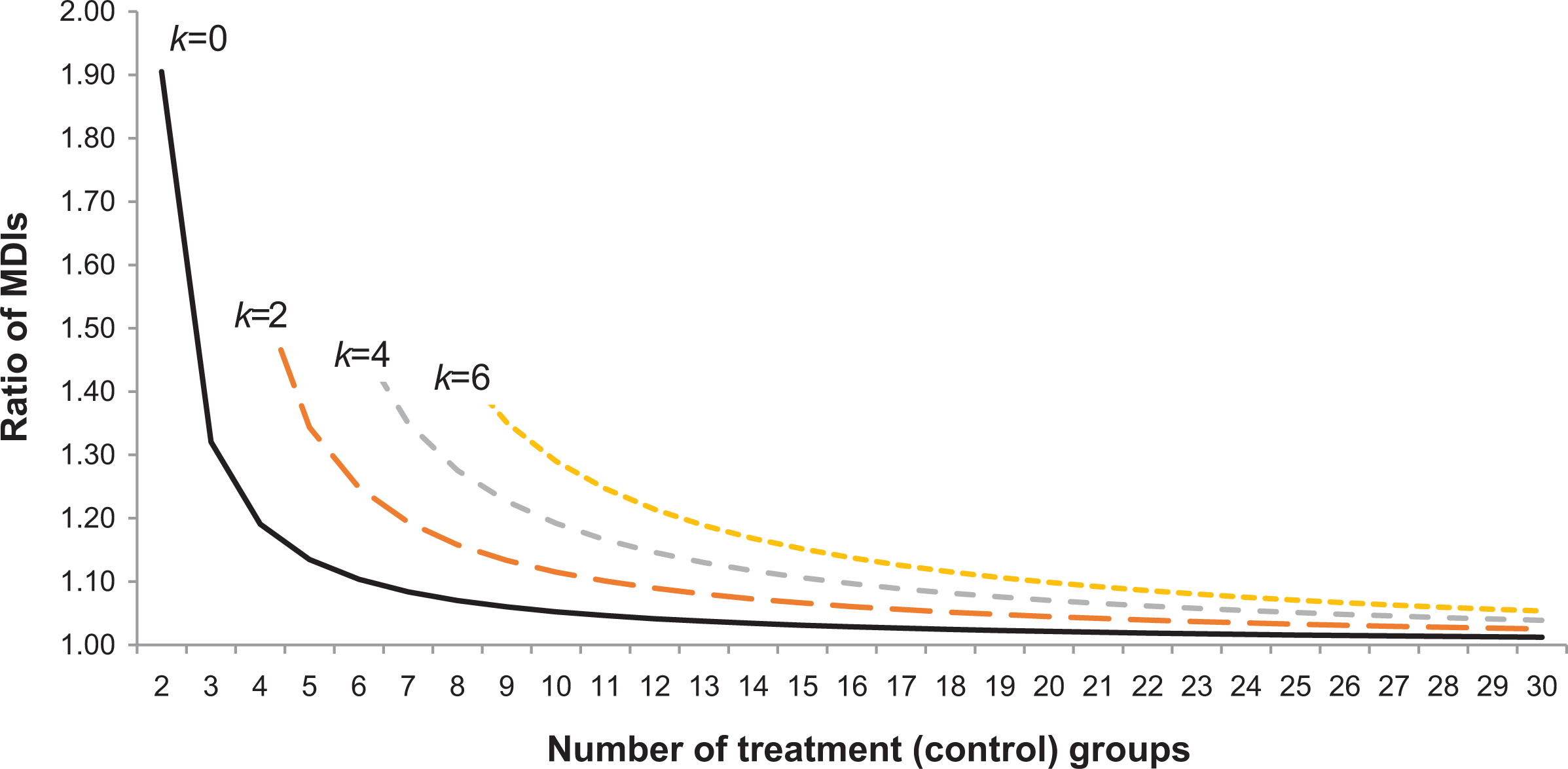
The results shown in Figure 1 (bottom solid line) and Appendix Table 1 in the online version of the article suggest that MDI increases using the grouped data (design effects) are less than 5% if there are at least 10 treatment and 10 control groupings ( $d f = 18$ ). MDI increases are 32% for 6 total groupings, 13% for 10 groupings, 5% for 20 groupings, and 2% for 40 groupings (design effects increase slightly at lower power levels). This means, for example, that if the RCT can detect an MDI of .20 standard deviations using the individual data, the MDI would increase to .21 using the grouped data with 20 total groupings. The results clearly show that MDI losses can be minimized by selecting more groupings and fewer individuals per group to the extent possible, as also noted by Prais and Aitchison (1954) for general regression models.

Figure 1.

Minimum detectable impact (MDI) ratios using randomly grouped and individual data for the nonclustered design, by the number of covariates (k). Notes: MDI calculations assume a 5% significance level at 80% power for a two-tailed test, a sample of 100 treatments and 100 controls, and groupings of equal size. See text for formulas.

Table 1.

Lower and Upper Confidence Intervals for t Statistics Based on Grouped Data as a Percentage of the “True” t Statistic Based on Individual Data

Number of Treatment/Control Groupings	90% Confidence Interval (Relative to the “True” t Statistic)		70% Confidence Interval (Relative to the “True” t Statistic)
Number of Treatment/Control Groupings	Lower Bound	Upper Bound	Lower Bound	Upper bound
10/10	.79	1.38	.86	1.23
20/20	.84	1.24	.90	1.14
30/30	.87	1.18	.92	1.11
40/40	.88	1.15	.93	1.09
50/50	.90	1.13	.93	1.08
100/100	.92	1.09	.95	1.06

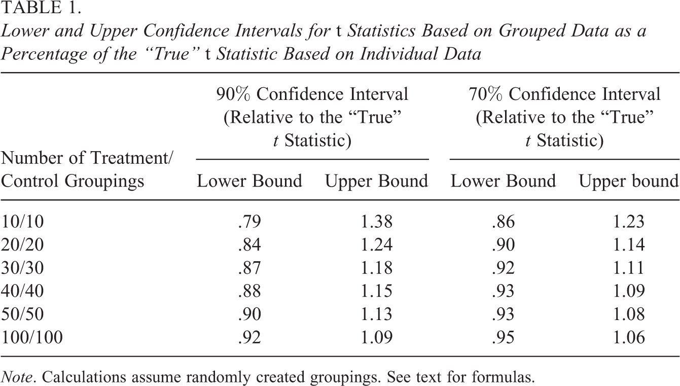
Note. Calculations assume randomly created groupings. See text for formulas.

A related metric for considering df losses using the grouped data is the reduced precision of the variance estimators. Applying asymptotic normality, we have using standard results that

\frac{S_{T G}^{2}}{G_{T}} \sim \frac{σ_{T I}^{2}}{Z G_{T} (G_{T} - 1)} χ^{2} (G_{T} - 1),

for the treatment group and similarly for the control group. Parallel expressions apply using the individual data. The variance of a χ² distribution is twice its df. Thus, if we replace $G_{T}$ and $G_{C}$ with an average value, $\bar{G}$ , we can use Equation 11 to approximate the precision of the variance estimator as $2 (σ_{T I}^{4} + σ_{C I}^{4}) / Z^{2} {\bar{G}}^{2} (\bar{G} - 1)$ using the grouped data and $2 (σ_{T I}^{4} + σ_{C I}^{4}) / Z^{2} {\bar{G}}^{2} (Z \bar{G} - 1)$ using the individual data. Thus, precision will be about Z times smaller using the grouped data, thereby increasing the dispersion of t statistics (and p values) across different possible groupings.

A useful way to measure the risk of using grouped data is to quantify the extent to which t statistics (and p values) match the “true” values based on the individual data. To do this, note that t statistics vary across different possible groupings of the individual data only because of variation in the estimated standard errors (the estimated impacts remain constant across all groupings).¹ Thus, we can create confidence intervals for the group-based t statistics—conditional on the t statistics for the individual data—using confidence intervals for the standard errors based on Equation 11. If we replace $G_{T}$ and $G_{C}$ with $\bar{G}$ and assume $σ_{T I}^{2} = σ_{C I}^{2} = σ_{I}^{2}$ , we find using Equation 11 that $(1 - α)$ % confidence intervals as a ratio of the “true” t statistic based on the individual data can be approximated using $\sqrt{2 (\bar{G} - 1)} / \sqrt{{ChiSq}_{θ}^{- 1} (2 \bar{G} - 2)}$ , where ${ChiSq}_{θ}^{- 1} (2 \bar{G} - 2)$ is the inverse of the chi-squared distribution with $(2 \bar{G} - 2)$ df and left probability $θ = α / 2$ for the upper bound and $θ = 1 - (α / 2)$ for the lower bound.²

Using this formula, Table 1 displays confidence intervals for group-level t statistics as a ratio of “true” values based on the individual data. The table shows that with 30 treatment and 30 control groupings (60 total), there is a 90% chance that the grouped-based t statistic will lie between 87% and 118% of the “true” t statistic. This means that if the “true” t statistic is less than 1.69 or greater than 2.31, findings regarding statistical significance will very likely be the same using the grouped data and the individual data. The 70% confidence interval bounds narrow to 92% and 111% of the “true” t statistic, respectively. These findings suggest that risks associated with using grouped data in terms of overall study conclusions regarding statistical significance appear to be tolerable, even if the number of groups is relatively small.

One strategy for reducing the statistical risks of using grouped data is to obtain Q replications of the grouped data rather than just one and to average the estimated ATEs and variances across replications. To examine how this “meta-analysis” approach reduces the sampling error of the estimated variances around the “true” variance based on the individual data, suppose we were to first enumerate the universe of all possible combinations of $G_{T}$ groupings of size Z for the treatment group and then estimate the variance for each one. The mean of these treatment group variances will equal the “true” variance based on the individual data and similarly for the control group. Intuitively, no information is lost from grouping if we knew the variances for each possible combination. Thus, obtaining Q replications of the grouped data is essentially a simple random sample from the universe of all possible combinations of groupings. Accordingly, the resulting sampling error of the mean of the Q variances around the “truth” will be reduced by about Q relative to the sampling error of the variance based on a single replication only. This means that effective sample sizes for computing the confidence intervals for the t statistics above will increase by a factor of Q. For example, if $Q = 2$ , sampling error of the variance around the “true” variance will be halved relative to a design with $Q = 1$ , and effective sample sizes for the confidence interval computations will double.³ These gains are demonstrated in Section 4 using data from a real-world education RCT.

2.3. Extensions to FP Models

Under the FP model, the sample and their potential outcomes are assumed to be fixed for the study, so the impact results are assumed to pertain to the study sample only and not more broadly as in the SP framework. The FP scenario could be realistic when the sample is purposively selected for the study (e.g., study volunteers). In the FP model, the only source of randomness is $T_{i}$ , and the ATE parameter of interest is $β_{1, F P} = \sum_{i = 1}^{N} (Y_{i} (1) - Y_{i} (0)) / N$ .

Under the FP model, the relation in Equation 1 still holds, and we can create a similar regression model as in Equation 2 using sample averages rather than population ones. This model is more complex than the SP model because the error term does not have mean zero over the randomization distribution, R, is heteroscedastic and is correlated with the regressor $(T_{i} - p)$ . Freedman (2008), Schochet (2010), and Li and Ding (2017) show that the OLS estimator using this model, ${\hat{β}}_{1, F P} = ({\bar{y}}_{T} - {\bar{y}}_{C})$ , is unbiased and asymptotically normal as N approaches infinity for an increasing sequence of FPs and that the variance can be conservatively estimated as follows:

{Var}_{R} ({\hat{β}}_{1, F P}) = \frac{S_{T}^{2}}{N_{T}} + \frac{S_{C}^{2}}{N_{C}} - \frac{{(S_{T} - S_{C})}^{2}}{N} .

The numerator in the final term in Equation 12 is a lower bound on the heterogeneity of treatment effects across the sample, $S_{τ}^{2} = \sum_{i = 1}^{N} {[(Y_{i} (1) - \bar{Y} (1)) - (Y_{i} (0) - \bar{Y} (0))]}^{2} / (N - 1)$ , which is not identified.

To develop FP estimators using group-level averages only, we can follow a parallel approach as for the SP model. The OLS estimator is the same as for the SP model, and the group-level variance can be estimated using

{V \hat{a} r}_{R} ({\hat{β}}_{G, F P}) = \frac{S_{T G}^{2}}{G_{T}} + \frac{S_{C G}^{2}}{G_{C}} - \frac{{(\sqrt{Z} S_{T G} - \sqrt{Z} S_{C G})}^{2}}{N} .

Design effects using grouped versus individual data are similar for the FP and SP models.

2.4. Incorporating Weights

Let $w_{i g}$ be the weight for individual i in group g, and let $w_{g} = \sum_{i}^{} w_{i g}$ be the aggregate weight in group g. For weighted analyses, we assume data are released on ${\bar{y}}_{g W}$ , $T_{g}$ , $Z_{g}$ , and $w_{g}$ for each group, where ${\bar{y}}_{g W} = \frac{1}{w_{g}} \sum_{i}^{} w_{i g} y_{i g}$ is the weighted mean for group g.

For analyses using grouped data, weighted least squares (WLS) methods using the weights, $w_{g}$ , should typically be used for two reasons. First, weights can adjust for biases due to groups that contain fewer than Z individuals due to rounding. For instance, if $N_{T} = 103$ and $G_{T} = 10$ , the grouped data will contain 10 groups with 10 treatments and an 11th group with only three individuals. Second, using weights will ensure that estimates of the treatment group assignment rate, $\hat{p}$ , will be the same using the grouped and individual data, which will matter for the more complex designs considered later. If relevant, weights can also help adjust for potential biases due to data nonresponse and other design-related factors as with individual data. Thus, we only consider WLS estimators hereafter and use the W subscript to indicate weighted statistics.

The WLS impact estimator for the grouped data using Equation 7 is ${\hat{β}}_{1 G W} = {\bar{\bar{y}}}_{T G W} - {\bar{\bar{y}}}_{C G W}$ , where ${\bar{\bar{y}}}_{T G W} = \frac{1}{G_{T} {\bar{w}}_{T G}} \sum_{g : T_{g} = 1}^{G_{T}} w_{g} {\bar{y}}_{g W}$ , ${\bar{\bar{y}}}_{C G W} = \frac{1}{G_{C} {\bar{w}}_{C G}} \sum_{g : T_{g} = 0}^{G_{C}} w_{g} {\bar{y}}_{g W}$ , ${\bar{w}}_{T G} = \frac{1}{G_{T}} \sum_{g : T_{g} = 1}^{G_{T}} w_{g}$ , and ${\bar{w}}_{C G} = \frac{1}{G_{C}} \sum_{g : T_{g} = 0}^{G_{C}} w_{g}$ . This estimator is the same as using the individual data. Using results in Schochet (2015/2016), this WLS estimator is consistent and asymptotically normal (conditional on the weights), and the group-level variance for the SP model can be estimated as follows:

{V \hat{a} r}_{R I} ({\hat{β}}_{1 G W}) = \frac{S_{T G W}^{2}}{G_{T}} + \frac{S_{C G W}^{2}}{G_{C}},

where

S_{T G W}^{2} = \frac{1}{(G_{T} - 1) {\bar{w}}_{T G}^{2}} \sum_{g : T_{g} = 1}^{G_{T}} w_{g}^{2} {({\bar{y}}_{g W} - {\bar{\bar{y}}}_{T G W})}^{2}; S_{C G W}^{2} = \frac{1}{(G_{C} - 1) {\bar{w}}_{C G}^{2}} \sum_{g : T_{g} = 0}^{G_{C}} w_{g}^{2} {({\bar{y}}_{g W} - {\bar{\bar{y}}}_{C G W})}^{2},

and similarly for the FP model in Equation 12.

The losses in statistical information using grouped data (randomly formed) rather than individual data are similar using weighted and unweighted data. The key reason is that design effects due to weighting are similar in expectation using the grouped and individual data. Design effects for the treatment group are $G_{T} \sum_{g : T_{g} = 1}^{G_{T}} w_{g}^{2} / (\sum_{g : T_{g} = 1}^{G_{T}} w_{g})^{2}$ for the grouped data and $N_{T} \sum_{i : T_{i} = 1}^{N_{T}} w_{i}^{2} / (\sum_{i : T_{i} = 1}^{N_{T}} w_{i})^{2}$ for the individual data and similarly for the control group. With random sorting, these ratios converge to the same value as the number of groups increases.

2.5. Blocked Designs

The methods above pertain also to blocked designs where random assignment is conducted separately within partitions of the entire sample (e.g., by site). For blocked designs, the design-based ATE parameter of interest is the weighted average of the ATE parameters in each block (e.g., using block sample sizes as weights). Schochet (2015/2016) discusses details of these estimators for individual data, which are shown to be asymptotically normal. Thus, t tests with $\sum_{b = 1}^{h} (N_{T b} + N_{C b}) - 2 h$ degrees of freedom can be used for hypothesis testing, where h is the number of blocks and $N_{T b}$ and $N_{C b}$ are respective treatment and control group sample sizes in block $b (b = 1, . . ., h)$ .

To apply these design-based methods to grouped data, we assume that random groupings are formed for each block, separately for treatments and controls, and that the number of groupings per block is proportional to block sample sizes. We assume that data are released on ${\bar{y}}_{b g W}$ , $T_{b g}$ , $Z_{b g}$ , $w_{g b}$ , and $Γ_{b g}$ for each grouping, where $Γ_{b g}$ are indicator variables of block membership.

Design-based estimators can then be obtained by regressing the ${\bar{y}}_{b g W}$ observations on block-by-treatment status interaction terms ( $Γ_{b g} T_{b g}$ ) and block indicators ( $Γ_{b g}$ ). The estimated parameters on the interaction terms measure the block-specific impacts, and these impacts and their variances can then be averaged to obtain pooled impact and variance estimators.⁴ Hypothesis testing can be conducted using t tests with $\sum_{b = 1}^{h} (G_{T b} + G_{C b}) - 2 h$ degrees of freedom, where $G_{T b}$ and $G_{C b}$ are the number treatment and control groups in block b. Hence, df losses using grouped data are slightly worse for blocked designs than nonblocked designs (assuming the same number of total groupings) because the $2 h$ term will matter more using the grouped data. Thus, slightly more groupings for blocked designs may be needed to compensate for these losses.

Alternatively, the model could only include $T_{b g}$ and $Γ_{b g}$ but not the interaction terms, in which case the estimated parameter on $T_{b g}$ measures the pooled ATE estimator. This approach provides a more parsimonious specification and, in general, more precise impact estimates but will typically yield biased estimates of the ATE parameter under the blocked design (see Schochet, 2015/2016). The df for this estimator using the grouped data is $\sum_{b = 1}^{h} (G_{T b} + G_{C b}) - h - 1$ .

2.6. Models With Covariates

In RCTs, baseline (preintervention) covariates are often included in the regression models to improve precision and to control for random treatment-control imbalances. Let $x_{i}$ denote a $1 x k$ vector of baseline covariates, unaffected by the treatment, drawn from SP distributions with finite first and second moments. In the design-based framework, the covariates are not part of the true model in Equation 2, and the ATE parameter, $β_{1}$ , still pertains to the model with covariates. If the covariates have any explanatory power, they will be correlated with the error term in Equation 2. We do not need to assume that the true conditional distribution of $y_{i}$ given $x_{i}$ is linear in $x_{i}$ .

With covariates, we now assume that data are released on ${\bar{y}}_{g W}$ , $T_{g}$ , $Z_{g}$ , $w_{g}$ , and ${\bar{x}}_{g W}$ for each randomly formed grouping, where ${\bar{x}}_{g W l} = \frac{1}{w_{g}} \sum_{i}^{} w_{i g} x_{i g l}$ is the weighted mean for covariate l in group g. Consider using WLS methods on the grouped data to regress ${\bar{y}}_{g}$ on the explanatory variables, ${\bar{z}}_{g W} = (1 T_{g} {\bar{x}}_{g W})$ , with respective parameters, $β_{0 W, MR}$ , $β_{1 W, MR}$ , and $γ_{W}$ (note that including $T_{g}$ or $(T_{g} - p)$ yields the same results and that Equation 7 remains the true model). Using design-based asymptotic results for multiple regression (MR) estimators based on individual-level data (see, e.g., Freedman, 2008; Imbens & Rubin, 2015; Schochet, 2010, 2015/2016; Yang & Tsiatis, 2001), we find that the WLS estimator using the grouped data, ${\hat{β}}_{1 G W, MR} = {[{(\sum_{g = 1}^{G} w_{g} {\bar{z}}^{'}_{g W} {\bar{z}}_{g W})}^{- 1} \sum_{g = 1}^{G} w_{g} {\bar{z}}^{'}_{g W} {\bar{y}}_{g W}]}_{2, 2}$ , is consistent and asymptotically normal. This estimator will typically differ from the WLS estimator using the individual data (but both are consistent).

Schochet (2015/2016) shows that a variance estimator based on model residuals that perform well in simulations (in generating Type 1 errors near nominal values and matching true standard errors) is as follows:

{V \hat{a} r}_{R I} {(\hat{β}}_{1 G W, MR}) = \frac{1}{(1 - R_{T X W}^{2})} [\frac{{MSE}_{T G W}}{G_{T}} + \frac{{MSE}_{C G W}}{G_{C}}],

where

{MSE}_{T G W} = \frac{1}{(G_{T} - k {\hat{p}}_{W} - 1) {\bar{w}}_{T G}^{2}} \sum_{g : T_{g} = 1}^{G_{T}} w_{g}^{2} {({\bar{y}}_{g W} - {\hat{β}}_{0 W, MR} - {\hat{β}}_{1 W, MR} - {\bar{x}}_{g W} {\hat{γ}}_{W})}^{2};

{MSE}_{C G W} = \frac{1}{(G_{C} - k (1 - {\hat{p}}_{W}) - 1) {\bar{w}}_{C G}^{2}} \sum_{g : T_{g} = 0}^{G_{C}} w_{g}^{2} {({\bar{y}}_{g W} - {\hat{β}}_{0 W, MR} - {\bar{x}}_{g W} {\hat{γ}}_{W})}^{2};

${\hat{β}}_{0 W, MR}$ , ${\hat{β}}_{1 W, MR}$ , and ${\hat{γ}}_{W}$ are parameter estimates, and $R_{T X W}^{2}$ is the $R^{2}$ value from a weighted regression of $T_{g}$ on $(1 {\bar{x}}_{g W})$ that captures finite-sample, treatment-control covariate imbalance. Hypothesis testing can be conducted using t tests with $(G - k - 2)$ degrees of freedom, where $G = G_{T} + G_{C}$ is the total number of groups.

With covariates, the statistical cost of using the grouped data rather than the individual data is 2-fold: (1) $d f$ losses, where more groups are now required to compensate for the number of covariates, k, to minimize power losses and (2) larger expected $R_{T X W}^{2}$ values, which increase variances. To quantify the $R_{T X W}^{2}$ inflation, we can apply asymptotic normality to approximate $R_{T X W}^{2}$ as $k F / [(G - k - 1) + k F]$ , where $F \sim F (k, G - k - 1)$ is the usual F statistic to gauge the statistical significance of the covariates in the regression of $T_{g}$ on $(1 {\bar{x}}_{g W})$ . This F ratio is distributed as $Beta (k / 2, (G - k - 1) / 2)$ with mean $k / (G - 1)$ (Johnson, Kotz, & Balakrishnan, 1994). Thus, a first-order approximation for the variance inflation adjustment factor in Equation 16 is ${(1 - E (R_{T X W}^{2}))}^{- 1} = (G - 1) / (G - k - 1)$ using the grouped data, compared to $(N - 1) / (N - k - 1)$ using the individual data.

These inflation factors can matter if the number of groupings is small: for example, with two covariates ( $k = 2$ ), the inflation factor is 11.8% for $G_{T} = G_{C} = 10$ compared to 1% for $N_{T} = N_{C} = 100$ , but for $k = 4$ , the corresponding inflation factors are 26.7% and 2.1%.⁵ Note that the inflation factors might not apply to QEDs where matching is used to balance the covariates. Note also that the expected total model $R^{2}$ value does not change with randomly formed groupings.

Figure 1 and Appendix Table 1 in the online version of the article show MDI increases using the grouped data relative to the individual data for models with covariates ( $k = 2, 4, 6$ ). The MDI ratios are calculated using the formula in Equation 10, incorporating both $d f$ losses and $R_{T X W}^{2}$ increases. The results indicate that MDI increases are expected to be less than 5% if the sample contains at least 38 total groups (19 treatment and 19 control) for $k = 2$ , at least 52 total groups for $k = 4$ , and at least 62 total groups for $k = 6$ . Thus, if the number of allowable groups is limited, it is important to include only a small number of covariates in the model (such as preintervention measures of the outcomes) to minimize design effects.

Forming groupings by a single covariate (or combinations of multiple covariates) rather than randomly can reduce design effects due to $R_{T X W}^{2}$ increases (but other model features remain). To see this, note that for any grouping mechanism, the total residual sum of squares from regressing $T_{i}$ on $(1 x_{i})$ using the individual data can be decomposed into between- and within-group components. Forming groups by covariate values will increase the between-group component with an offsetting decrease in the within-group component, which means that less information is lost by grouping. For example, if the model contains a single categorical covariate with few categories, grouping by that covariate would yield negligible design effects. Sorting randomly leads to maximum information loss.

The gains from covariate-based grouping will largely depend on the number and joint distributions of the covariates. Simulations shown in Appendix B in the online version of the article (for a parallel setting for clustered designs discussed in Section 3) suggest that these gains can be quantified using the intraclass correlation coefficient (ICC) of the predicted values ( $ρ_{p}$ ) across groupings based on the individual regression of $T_{i}$ on $(1 x_{i})$ . The approach involves replacing G in the $R_{T X W}^{2}$ formula by the effective sample size, $G^{*} = G [1 + ρ_{p} (\bar{Z} - 1)]$ , where $\bar{Z}$ is the mean group size. If $ρ_{p} = 1$ , we have $G^{*} = N$ (maximal gain) and $G^{*} = G$ if $ρ_{p} = 0$ (no gain). This $G^{*}$ formula is motivated by the effective sample size formula for clustered designs in Kish (1995).

Note that with covariate-based grouping, the estimation model must include the covariates used to construct the groupings or biases can result. Thus, this grouping scheme may not be suitable for all analyses and should be used cautiously. Grouping by covariates will have a much larger effect on reducing the standard errors of the grouping variables themselves and other model covariates with which they are correlated.

Finally, we note that with covariates, regardless of the sorting mechanism, the grouped data can fully replicate the design-based impact and variance estimators based on the individual data if the following additional weighted statistics are requested for each group g and covariate l: $\sum_{i} w_{i g} x_{i g l} y_{i g}$ , $\sum_{i} w_{i g} x_{i g l} x_{i g l^{'}}$ , $\sum_{i} w_{i g}^{2}$ , $\sum_{i} w_{i g}^{2} y_{i g}^{2}$ , $\sum_{i} w_{i g}^{2} x_{i g l} y_{i g}$ , $\sum_{i} w_{i g}^{2} x_{i g l} x_{i g l^{'}}$ . These statistics, which involve weighted cross products of all covariates and outcomes, are required to estimate within-group variances. Their number can become large if the model contains many covariates.

2.7. Subgroup Analyses

In RCTs, analyses are often conducted to examine how intervention effects vary across baseline subgroups defined by individual and site characteristics. We consider categorical subgroups where each sample member is allocated to a discrete, mutually exclusive category. Aggregate statistics for each subgroup s could be included in the same groupings as for the full sample: ${\bar{y}}_{s g W}$ , $Z_{s g}$ , $w_{s g}$ , and ${\bar{x}}_{s g W}$ and subgroup indicators, $Λ_{s g}$ . However, with many subgroups, this approach can compromise data privacy, for example, if the sample contains only one individual with a specific combination of subgroup values and that individual is in a grouping that includes no other members with any of those subgroup values. To avoid this possibility, we assume separate groupings are created for each subgroup class; for example, we assume age subgroups are together in the same groupings but are separate from gender subgroups that are in their own groupings.

In this setting, the grouped estimation methods discussed in Subsection 2.5 for blocked designs apply fully to the subgroup analysis. For example, a common model specification would be to create separate group-level observations for each subgroup (e.g., for males and females) and estimate design-based models that include two-way interactions between the subgroup and treatment status indicators as well as subgroup indicators (see Schochet, 2015/2016, for details).

If many subgroup analyses are of interest, administrative data requests can become burdensome if separate groupings are requested for each subgroup class. A potentially appealing approach to minimize these data requests is to conduct the subgroup analysis using the G groupings for the full sample that also include data on subgroup proportions (such as the proportions of males and females) but not data on mean subgroup outcomes. Subgroup impacts can then be estimated using ecological regressions (Freedman et al., 1998; Goodman, 1959; King, 1997; Robinson, 1950). Importantly, we assume the full sample groupings are formed randomly, which ensures that the ecological regression approach produces unbiased estimates due to the independence of the model parameters and explanatory variables (see below). The ecological inference literature focuses on solutions to violations of this independence assumption that can cause bias, but we avoid these issues through random sorting of the data.

To examine this approach in our design-based context, we consider two subgroups, indexed by subscripts 1 and 2, where, for simplicity, we consider estimation without weights for the treatment group only (the same approach applies to the control group). To develop the ecological regression model, we first apply the design-based relations in Equations 2 and 7 for each subgroup assuming the same error variances. Second, we use the following relation:

{\bar{y}}_{g} = π_{1 g} {\bar{y}}_{1 g} + π_{2 g} {\bar{y}}_{2 g},

where $π_{1 g}$ is the proportion of group members in Subgroup 1 and $π_{2 g} = 1 - π_{1 g}$ is the proportion in Subgroup 2. This relation states that, for each grouping, the mean outcome for the full sample is a weighted average of the mean outcomes for the two subgroups (which are unobserved). If we next insert Equation 7 into Equation 17 for each subgroup, we obtain the following ecological regression model:

{\bar{y}}_{g} = π_{1 g} δ_{1} + π_{2 g} δ_{2} + {\bar{η}}_{g},

where $δ_{1} = β_{01} + β_{11} (1 - p)$ is the SP treatment mean for Subgroup 1, $δ_{2} = β_{02} + β_{12} (1 - p)$ is the SP treatment mean for Subgroup 2, and ${\bar{η}}_{g} = π_{1 g} {\bar{e}}_{1 g} + π_{2 g} {\bar{e}}_{2 g}$ is the error term with mean 0 and variance $σ_{T I}^{2} / Z$ . The goal is to estimate the parameters $δ_{1}$ and $δ_{2}$ .

Because the groupings are created randomly, $π_{1 g}$ and $π_{2 g}$ will be uncorrelated with $δ_{1}$ , $δ_{2}$ , and ${\bar{η}}_{g}$ . Thus, OLS applied to Equation 18 will yield unbiased estimates of $δ_{1}$ and $δ_{2}$ . Stated differently, by design, there are no ecological biases due to random sorting. To examine the precision of these ATE estimators, we compare the OLS variance of ${\hat{δ}}_{1}$ to the variance of the group-level estimator, $σ_{T I}^{2} / (G_{T} π_{1} Z)$ , from an alternative design where mean outcomes for Subgroup 1 are collected directly from $G_{T} π_{1}$ random groupings of Subgroup 1 members, where $π_{1}$ is the proportion of the full sample in Subgroup 1 (parallel results hold for Subgroup 2).

To calculate the OLS variance of ${\hat{δ}}_{1}$ , we use a first-order approximation described in Appendix A in the online version of the article. Using this formula, Table 2 displays MDI increases using the ecological regression approach relative to the direct collection of mean outcomes for the subgroups. The design effects can be large. For example, if $π_{1} = .5$ , the design effect is 1.73 if the group size (Z) is 5 and 3.24 if $Z = 20$ . This means, for example, that the MDI would increase from .20 to .35 standard deviations if $Z = 5$ and to .65 if $Z = 20$ . These results suggest that statistical power for estimating subgroup effects may be a serious concern using the ecological inference approach.

Table 2.

Minimum Detectable Impact Ratios for the Ecological Regression Approach Relative to Obtaining Mean Subgroup Outcomes Directly, for the Nonclustered Design

Proportion of Sample in Subgroup ( $π_{1}$ )	Size of Grouping (Z)
Proportion of Sample in Subgroup ( $π_{1}$ )	5	10	15	20
.3	1.95	2.70	3.29	3.78
.5	1.73	2.35	2.83	3.24
.7	1.48	1.92	2.28	2.59

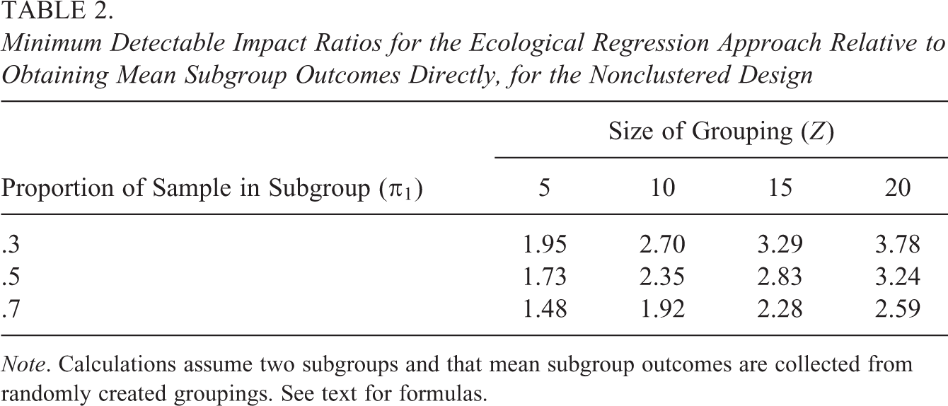
Note. Calculations assume two subgroups and that mean subgroup outcomes are collected from randomly created groupings. See text for formulas.

3. Clustered Designs

Clustered RCTs occur when clusters (such as schools or hospitals) are randomized rather than individuals. We assume the sample contains M total clusters with $M_{T} = M p$ treatment clusters and $M_{C} = M (1 - p)$ control clusters, where p is now the assignment rate of clusters to the treatment group. We adopt the same notation as for the nonclustered design, adding the subscript j to signify clusters. For example, $N_{j}$ is the number of individuals in the cluster, $T_{j}$ is the treatment indicator for the cluster, and $Y_{i j} (1)$ and $Y_{i j} (0)$ represent potential outcomes for individual i in cluster j in the treatment and control conditions. We assume SUTVA that (1) individuals’ potential outcomes depend on the treatment assignment of their cluster and not on those of others and (2) clusters and subjects can receive only one form of the treatment.

We focus on the SP design where it is assumed that study clusters and individuals are random samples from respective superpopulations, S, and I. The ATE parameter of interest is $β_{1, Clus} = μ_{T S} - μ_{C S}$ , where $μ_{T S}$ and $μ_{C S}$ are (finite) mean cluster-level potential outcomes in the S population for the treatment and control groups.

To develop consistent design-based estimators for $β_{1, Clus}$ using grouped data, we first highlight key features of design-based estimators for clustered designs using individual data following Schochet (2013, 2015/2016). Consider the data generating process for an individual’s observed mean outcome, $y_{i j}$ , that underlies clustered RCT designs:

y_{i j} = T_{j} Y_{i j} (1) + (1 - T_{j}) Y_{i j} (0) .

Rearranging this relation yields the following regression model generated by the experiment:

y_{i j} = β_{0, Clus} + β_{1, Clus} (T_{j} - p) + (u_{j, Clus} + e_{i j, Clus}),

where $β_{0, Clus} = p μ_{T S} + (1 - p) μ_{C S}$ , $u_{j, Clus} = T_{j} ({\bar{Y}}_{j} (1) - μ_{T S}) + (1 - T_{j}) ({\bar{Y}}_{j} (0) - μ_{C S})$ , and $e_{i j, Clus} = T_{j} (Y_{i j} (1) - {\bar{Y}}_{j} (1)) + (1 - T_{j}) (Y_{i j} (0) - {\bar{Y}}_{j} (0))$ .

This model is the usual random effects specification with mean zero between- and within-cluster error components that are uncorrelated with $(T_{j} - p)$ , but where the error variances differ for the treatment and control groups.

Unlike hierarchical linear modeling, the design-based (nonparametric) methods do not involve estimation of the variance components, but instead adjust WLS standard errors for clustering, similar to the generalized estimating equation approach with cluster-robust (sandwich) standard errors (Cameron & Miller, 2015; Liang & Zeger, 1986). Consider using WLS methods and the individual data to regress $y_{i j}$ on the explanatory variables, $(1 T_{j} x_{i j})$ , with respective parameters, $β_{0, Clus}$ , $β_{1, Clus}$ , and $γ_{C l u s}$ , where $x_{i j}$ is a $1 x k$ vector of covariates. Note that Equation 20 remains the true model. The covariates can be at the individual or cluster level. Schochet (2013, 2015/2016) and results in Li and Ding (2017) show that under certain regularity conditions, as M increases to infinity, the MR estimator, ${\hat{β}}_{1, W, MR, Clus}$ , is asymptotically normal with asymptotic mean, $β_{1, Clus}$ . A consistent variance estimator is

{V \hat{a} r}_{IRS} ({\hat{β}}_{1, W, MR,Clus}) = \frac{1}{(1 - R_{T X W, Clus}^{2})} [\frac{{MSE}_{T, Clus}}{M_{T}} + \frac{{MSE}_{C, Clus}}{M_{C}}],

where

{MSE}_{T, Clus} = \frac{1}{(M_{T} - k \hat{p} - 1) {\bar{w}}_{T}^{2}} \sum_{j : T_{j} = 1}^{m_{T}} w_{j}^{2} {({\bar{y}}_{j W} - {\hat{β}}_{0, Clus} - {\hat{β}}_{1, Clus} - {\bar{x}}_{j W} {\hat{γ}}_{C l u s})}^{2},

{MSE}_{C, Clus} = \frac{1}{(M_{C} - k (1 - \hat{p}) - 1) {\bar{w}}_{C}^{2}} \sum_{j : T_{j} = 0}^{m_{C}} w_{j}^{2} {({\bar{y}}_{j W} - {\hat{β}}_{0, Clus} - {\bar{x}}_{j W} {\hat{γ}}_{C l u s})}^{2},

${\bar{w}}_{T} = \sum_{j : T_{j} = 1}^{m_{T}} w_{j} / M_{T}$ and ${\bar{w}}_{T} = \sum_{j : T_{j} = 0}^{m_{C}} w_{j} / M_{C}$ are mean cluster-level weights, $R_{T X W, Clus}^{2}$ is from a regression of $T_{j}$ on the covariates and an intercept, and $\hat{p} = \sum_{j = 1}^{M} T_{j} w_{j} / \sum_{j = 1}^{M} w_{j}$ is the weighted proportion of clusters in the treatment group. Hypothesis testing can be conducted using t tests with $(M - k - 2)$ degrees of freedom, which is based on the number of clusters, not the number of individuals.

Importantly, the variance estimator in Equation 21 is based on individual-level model residuals that are averaged to the cluster level. Stated differently, the model is estimated using the individual data, but the $MSE$ terms for calculating standard errors are based on values for ${\bar{y}}_{j W}$ , ${\bar{x}}_{j W}$ , and $w_{j}$ (i.e., data aggregated to the cluster level).

These results suggest that for clustered designs, a natural grouping scheme is to request administrative data by cluster—for example, school- or hospital-level averages—to minimize information loss. Under this scheme, data would be requested on ${\bar{y}}_{g W}$ , $T_{g}$ , $Z_{g}$ , $w_{g}$ , and ${\bar{x}}_{g W}$ for each cluster. In essence, the clusters become the groupings. Because of linearity of the relationship in Equation 20, the same model and error structure as in Equation 20 holds at the cluster level. Thus, the estimation of the regression model using the grouped data will yield consistent impact estimators, and Equation 21 can be used for variance estimation. The use of cluster-level averages to analyze clustered RCT data has a long history across many disciplines even if individual-level data are available (e.g., Campbell, Mollison, Steen, Grimshaw, & Eccles, 2000; Fleiss, 1986; Gerber & Green, 2012; Murray, 1998). A key difference using design-based estimation is that randomization yields separate variances for the treatment and control groups.

Importantly, for models without covariates or with cluster-level covariates only, analyzing data averaged to the cluster level yields the same design-based impact and variance estimators with the same df as using the individual data, so no information is lost. However, if the model includes individual-level covariates (that vary both within and between clusters), the ATE and variance estimators will differ using the grouped and individual data (but both are consistent).⁶ In this case, grouping by clusters will yield larger expected $R_{T X W, Clus}^{2}$ values than using the individual data, so are less efficient. Simulation evidence in Appendix B in the online version of the article suggests that these design effects can be closely approximated by $[1 - \frac{k}{(N^{*} - 1)}] / [1 - \frac{k}{(M - 1)}]$ , where $N^{*} = N / [1 + ρ_{p} (\bar{N} - 1)]$ , $\bar{N}$ is the average cluster size, and $ρ_{p}$ is the ICC of the predicted values from the regression of $T_{j}$ on the covariates using the individual data. This ICC measures how much of the total variation in the covariates is due to variation between clusters. As $ρ_{p}$ approaches 0, $N^{*}$ approaches N (maximum design effects), whereas if $ρ_{p} = 1$ , $N^{*} = M$ (no design effects).

Table 3 displays design effects using our approximation assuming equal numbers of treatment and control group clusters. For $k = 2$ , if $ρ_{p} = .05$ , at least 20 total clusters are required to yield design effects of less than 5%, but only 14 clusters are required if $ρ_{p} = .5$ . Design effects increase markedly as k increases, suggesting that researchers should limit the number of covariates for analyses based on cluster-level averages.

Table 3.

Minimum Detectable Impact Ratios Using Cluster-Level Averages Relative to Individual Data for Models With Individual-Level Covariates, for Clustered Designs

Total Number of Clusters $(M)$	ICC of Predicted Values From the Regression of Treatment Status on the Covariates Using the Individual Data $(ρ_{p})$
Total Number of Clusters $(M)$	0.05	0.2	0.5
Number of covariates, $k = 2$
6	1.28	1.24	1.16
10	1.13	1.11	1.07
20	1.05	1.05	1.03
30	1.03	1.03	1.02
40	1.02	1.02	1.01
60	1.02	1.01	1.01
Number of covariates, $k = 6$
10	1.70	1.61	1.43
20	1.20	1.17	1.11
30	1.12	1.10	1.06
40	1.08	1.07	1.04
60	1.05	1.04	1.03

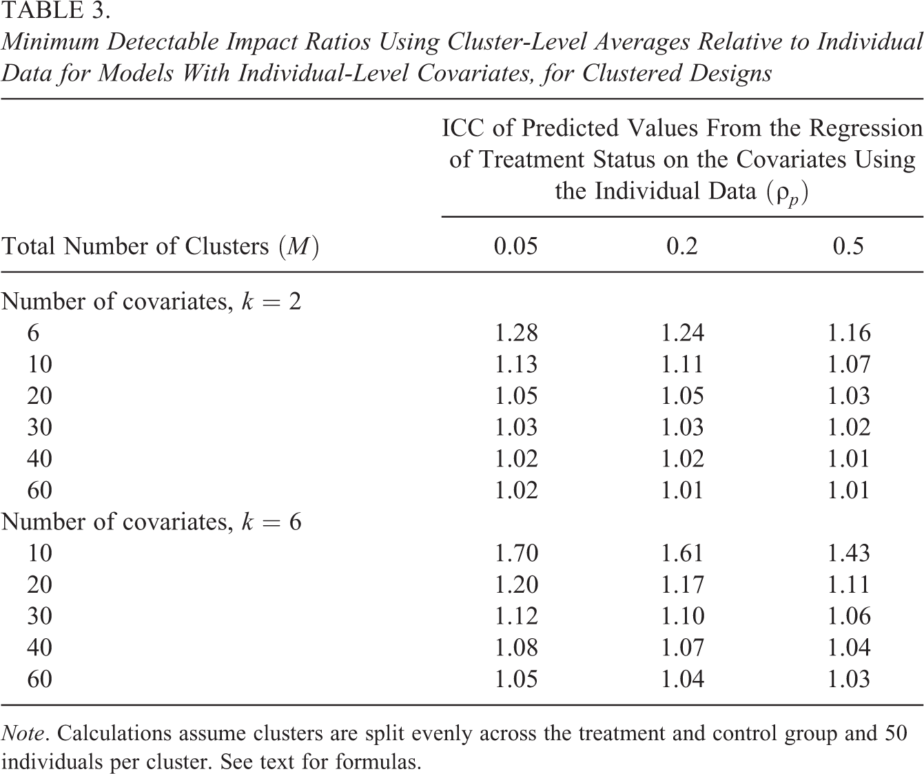
Note. Calculations assume clusters are split evenly across the treatment and control group and 50 individuals per cluster. See text for formulas.

Note that design effects can be reduced if additional groupings are formed by sorting individuals into groupings within each cluster, either randomly or by covariates. If this sorting is random, design effects can be approximated using $[1 - \frac{k}{(N^{*} - 1)}] / [1 - \frac{k}{(M \bar{G} - 1)}]$ , where $\bar{G}$ is the average number of groupings per cluster.

Finally, regardless of the sorting mechanism, the grouped data for clustered designs can fully replicate the design-based impact and variance estimators based on the individual data if the following additional weighted statistics are requested for each group g and covariate l: $\sum_{i} w_{i g} x_{i g l} y_{i g}$ , $\sum_{i} w_{i g} x_{i g l} x_{i g l^{'}}$ , $\sum_{i} w_{i g}^{2}$ , $\sum_{i} w_{i g}^{2} y_{i g}^{2}$ , $\sum_{i} w_{i g}^{2} x_{i g l} y_{i g}$ , $\sum_{i} w_{i g}^{2} x_{i g l} x_{i g l^{'}}$ . These statistics allow for estimation of within-group variances that are needed to fully replicate the estimators using the individual-level data.

4. Empirical Analysis

To examine how the theory using the grouped data applies in practice, we analyzed data from two RCTs in the education field, one that used a nonclustered design and the other that used a clustered design. The nonclustered RCT—the New York City School Voucher Experiment (Mayer, Peterson, Myers, Tuttle, & Howell, 2002)—examined the effects of offering scholarships to private schools worth up to US$1,400 a year for 3 years to children from low-income families. Eligible students who applied for scholarships were randomly selected for the treatment group using a lottery system. The clustered RCT—the Teach for America Evaluation (Decker, Glazerman, & Mayer, 2004)—examined the impacts of the Teach for America (TFA) Program that recruits seniors and recent graduates with strong academic records from selective colleges to teach for a minimum of 2 years in low-income schools. Students were randomly assigned to classrooms (clusters) taught by TFA teachers or traditional teachers in the same schools. Table 4 describes the studies, including the samples, outcome variables, and baseline covariates for the analysis. Our goal is not to mimic the original study findings or to provide policy conclusions but to demonstrate several key features of ATE estimation using grouped data to demonstrate the theory developed above.

Table 4.

Summary of Randomized Controlled Trial Data for the Empirical Analysis

Evaluation	Sample	Outcomes and Covariates for the Analysis
New York City School Voucher Experiment (Mayer et al. 2002)	Low-income children enrolled in kindergarten to fourth grade in 1997 in New York City public schools 781 treatments; 675 controls	Outcome: Iowa Test of Basic Skills (ITBS) math scores in spring 2000 (651 treatments and 527 controls with nonmissing data) Covariates: Baseline ITBS math test scores, grade, whether in a special education or gifted grade, and race and ethnicity
Teach for America Evaluation (Decker et al. 2004)	First to fifth graders in the 2001–2002 school year; 17 schools in five cities Teachers: 43 treatment; 53 control Students: 1,014 treatment; 815 control	Outcome: Iowa Test of Basic Skills (ITBS) math scores in spring 2002 (720 treatments and 910 controls with nonmissing data) Covariates: Baseline ITBS math scores, grade, race and ethnicity, and eligibility for free or reduced-price lunch

Table 5 presents empirical results for the NYC Voucher experiment using the individual and grouped data. The table shows estimated ATEs, standard errors, and p values for models without covariates, those with the pretest covariate only, and those with the full set of 11 covariates. Groups of size 5, 10, 20, and 50 individuals were formed randomly, separately for treatments and controls.⁷ We generated 500 random groupings and report mean statistics as well as 5th and 95th percentiles of the p values to gauge the risks of obtaining different conclusions regarding statistical significance using the grouped and individual data. We conducted the analysis assuming one set of groupings and averaging across five sets of groupings to improve power.

Table 5.

Full-Sample Impact Estimation Results for the New York City Voucher Experiment

Sample	Model Without Covariates		Model with Pretest Covariate Only		Model with all 11 Covariates
Sample	Impact (Standard Error)^a	p Value^b	Impact (Standard Error)^a	p Value^b	Impact (Standard Error)^a	p Value^b
Individual data	−1.59 (1.37)	.25	−1.78 (1.18)	.13	−1.71 (1.15)	.14
Grouped data: Group size; number of treatment/control groupings
5; 131/106	−1.59 (1.36)	.25 .21–.28 .23–.26	−1.78 (1.18)	.13 .10–.16 .12–.15	−1.70 (1.19)	.17 .07–.31 .11–.22
10; 66/53	−1.59 (1.36)	.25 .19–.30 .22–.27	−1.78 (1.18)	.13 .09–.18 .12–.15	−1.67 (1.23)	.20 .06–.44 .11–.27
20; 33/27	−1.59 (1.35)	.25 .17–.31 .21–.28	−1.78 (1.17)	.14 .08–.20 .10–.16	−1.72 (1.35)	.25 .04–.69 .10–.36
50; 14/11	−1.59 (1.35)	.25 .13–.36 .21–.30	−1.78 (1.16)	.14 .05–.23 .10–.18	−1.74 (1.72)	.38 .03–.90 .13–.69

Note. See text for a description of the data and formulas. Figures for the grouped data were obtained by randomly forming groups, separately for the treatment and control groups. The simulations were conducted for 500 replications (groupings).

^aFigures for the grouped data show mean impact and mean standard error estimates across 500 random groupings. ^bFigures for the grouped data show mean p values across 500 random groupings (first row) and the 5th and 95th percentiles for a single set of groupings (second row) and averaged across five sets of groupings (third row).

The results in Table 5 verify the theory that the point estimates for the ATEs using the grouped data are similar on average across the simulations to those using the individual data for models with and without covariates. Furthermore, all specifications show statistically insignificant school voucher effects.

For the models with covariates, standard error increases using the grouped data (because of higher $R_{T X W}^{2}$ values) are not noticeable if the model includes the pretest covariate only (Table 5). However, standard error increases are noticeable if the full set of 11 covariates are included, especially with few groupings. Relatedly, the p value spread (90% confidence interval) across simulated groupings is reasonably narrow if the model contains no covariates or the pretest covariate only, even if there are only 14 treatment and 11 control groupings. However, risks of finding different study conclusions using the grouped data increase substantially for the model with the full set of 11 covariates, which can be mitigated somewhat if five separate groupings are obtained rather than just one. These findings support the theory that only a few key covariates should be included in models using grouped data.

We also conducted a subgroup analysis for female students by estimating ecological regression models using full-sample groupings of size 10 (not shown). Across 500 simulations, this approach yielded standard errors 2.5 times larger than conducting the subgroup analysis using the individual data for females or separate groupings with mean outcomes for females, which is close to the 2.4 design effect predicted by theory (see Table 2).

Table 6 presents analysis results using data from the TFA study, where students are clustered within classrooms (teachers). Consistent with theory, the impact findings are identical using the individual- and cluster-level data for the model without covariates and for the model that includes the classroom-level pretest score only. For the latter model, we find that TFA teachers increased student math scores by an average of 2.68 scale points (0.14 effect size units), which is statistically significant. For the model with all 11 covariates, the impact results based on the individual and grouped data differ more. This finding is consistent with the theory that impact estimates using the grouped data become increasingly variable as the number of model covariates increase.

Table 6.

Full-Sample Impact Estimation Results for the Teach for America Evaluation

	Model Without Covariates		Model With Classroom-Level Pretests Only		Model With all 11 Covariates
Data	Impact (Standard Error)	p Value	Impact (Standard Error)	p Value	Impact (Standard Error)	p Value
Individual data	.82 (2.14)	.70	2.68 (1.14)	.02*	2.37 (1.08)	.03*
Classroom-level data	.82 (2.14)	.70	2.68 (1.14)	.02*	2.74 (0.99)	.01*

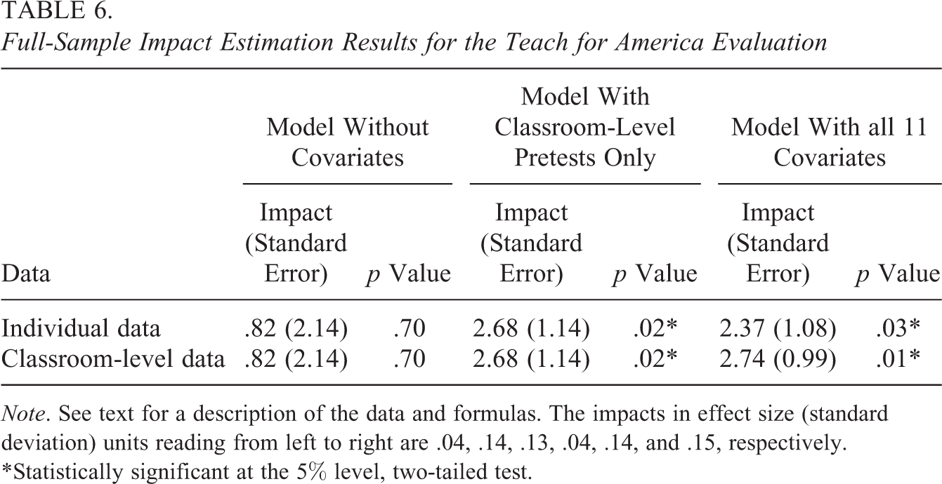
Note. See text for a description of the data and formulas. The impacts in effect size (standard deviation) units reading from left to right are .04, .14, .13, .04, .14, and .15, respectively.

*Statistically significant at the 5% level, two-tailed test.

5. Conclusions

This article has developed methods for quantifying the statistical costs of using group-level averages ( ${\bar{y}}_{g}$ , ${\bar{x}}_{g}$ , $w_{g}$ , $T_{g}$ , $Z_{g}$ ) to estimate ATEs for RCTs using administrative records data and design-based methods. For nonclustered designs, we focused on randomly formed groupings but also considered more efficient schemes with groupings based on baseline covariates. For clustered designs, we focused on schemes where groupings are cluster-level averages. Our main finding, supported by theory and empirical examples, is that using grouped data is a viable approach for impact estimation and thus could be an effective strategy to help gain access to administrative records data to avoid data disclosure.

We find that estimated impacts and standard errors using group-level averages have the same asymptotic statistical properties as those based on individual data. The key reason is that the individual-level regression model underlying experimental designs is linear and thus also holds at the grouped level for both (1) the nonclustered design, where groupings for the treatment and control groups are formed at random or by covariates included in the models, and (2) the clustered design, where groupings are formed as cluster-level averages or by individuals at random within clusters.

For the nonclustered design, the risks of using grouped data due to statistical power losses and the variability of impact results over the distribution of possible groupings are tolerable if the total number of groupings is about 40 or more, and the model includes only a few key covariates. The risks increase starkly as the number of covariates increases. If needed, obtaining multiple sets of groupings (and averaging impacts and variances over them) or forming groupings by sorting on covariates that are included in the models could be good strategies to minimize design effects. For the clustered design, little information is lost if administrative data are collected as cluster-level averages. In this case, there are no df losses, and standard error increases due to increased treatment-covariate correlations are minimal if the model contains only a few covariates. For all designs, conducting subgroup analyses using ecological regressions yields large design effects and is not recommended unless the study contains very large samples with excess statistical power; instead, separate groupings should be obtained for each subgroup. The free RCT-YES software (www.rct-yes.com) can be used to estimate impacts and standard errors for all designs considered in this article using grouped (or individual) data.

Supplemental Material

Supplemental Material, DS_10.3102_1076998619855350 - Analyzing Grouped Administrative Data for RCTs Using Design-Based Methods

Supplemental Material, DS_10.3102_1076998619855350 for Analyzing Grouped Administrative Data for RCTs Using Design-Based Methods by Peter Z. Schochet in Journal of Educational and Behavioral Statistics

Footnotes

Notes

References

Boruch

Reichen

(1975). Experimental testing of public policy. Boulder, CO: Westview.

Cameron

A. C.

Miller

D. L.

(2015). A practitioner’s guide to cluster-robust inference. Journal of Human Resources, 50, 317–372.

Campbell

M. K.

Mollison

Steen

Grimshaw

Eccles

(2000). Analysis of cluster randomized trials in primary care: A practical approach. Family Practice, 17, 192–196.

Card

Chetty

Feldstein

Saez

. (2010). Expanding access to administrative data for research in the U.S. (National Science Foundation 10-069 White Paper). Washington, DC: National Science Foundation.

Decker

Glazerman

Mayer

. (2004). The effects of teach for America on students: Findings from a national evaluation. Princeton, NJ: Mathematica Policy Research.

Dhrymes

Lleras-Muney

(2006). Estimation of models with group data by means of “2SLS.” Journal of Econometrics, 133, 1–29.

Feige

Watts

H. W.

(1972). An investigation of the consequences of partial aggregation of microeconomic data. Econometrica, 40, 343–360.

Fleiss

(1986). The design and analysis of clinical experiments. Chichester, England: Wiley.

Freedman

(2008). On regression adjustments to experimental data. Advances in Applied Mathematics, 40, 180–193.

10.

Freedman

Klein

S. P.

Ostland

Roberts

(1998). On “solutions” to the ecological inference problem (Statistics Department Working Paper). Berkeley: University of California.

11.

Gerber

Green

(2012). Field experiments: Design, analysis, and interpretation. New York, NY: W. W. Norton.

12.

Goodman

(1959). Some alternatives to ecological correlation. American Journal of Sociology, 64, 610–625.

13.

Holland

P. W.

(1986). Statistics and causal inference. Journal of the American Statistical Association, 81, 945–960.

14.

Imbens

Rubin

(2015). Causal inference for statistics, social, and biomedical sciences: An introduction. Cambridge, England: Cambridge University Press.

15.

Jacob

Goddard

Kim

E. S.

(2014). Assessing the use of aggregate data in the evaluation of school-based interventions: Implications for evaluation research and state policy regarding public use data. Educational Evaluation and Policy Analysis, 36, 44–66.

16.

Johnson

N. L.

Kotz

Balakrishnan

. (1994). Continuous univariate distributions (2nd ed.). New York, NY: Wiley Series in Probability and Statistics.

17.

King

(1997). A solution to the ecological inference problem. Princeton, NJ: Princeton University Press.

18.

Kish

(1995). Survey sampling. New York, NY: John Wiley.

19.

Ding

. (2017). General forms of finite population central limit theorems with applications to causal inference. Journal of the American Statistical Association, 112, 1759–1769.

20.

Liang

Zeger

(1986). Longitudinal data analysis using generalized linear models. Biometrika, 73, 13–22.

21.

Lin

(2013). Agnostic notes on regression adjustments to experimental data: Reexamining Freedman’s critique. Annals of Applied Statistics, 7, 295–318.

22.

Matthews

G. J.

Harel

(2011). Data confidentiality: A review of methods for statistical disclosure limitation and methods for assessing privacy. Statistics Surveys, 5, 1–29.

23.

Mayer

Peterson

Myers

Tuttle

Howell

(2002). School choice in New York City: An evaluation of the school choice scholarships program, Washington, DC: Mathematica Policy Research

24.

Miratrix

L. W.

Sekhon

J. B.

(2013). Adjusting treatment effect estimates in randomized experiments. Journal of the Royal Statistical Society B, 75, 369–396.

25.

Murray

D. M.

(1998). The design and analysis of group-randomized trials. Oxford, England: Oxford University Press.

26.

Neyman

(1923). On the application of probability theory to agricultural experiments: Essay on principles. Section 9, Translated in Statistical Science, 5, 465–472. (Original work published 1990)

27.

Prais

S. J.

Aitchison

(1954). The grouping of observations in regression analysis. Review of the International Statistical Institute, 22, 1–22.

28.

Robinson

W. S.

(1950). Ecological correlations and the behavior of individuals. American Sociological Review, 15, 351–357.

29.

Rubin

D. B.

(1974). Estimating causal effects of treatments in randomized and nonrandomized studies. Journal of Education Psychology, 66, 688–701.

30.

Rubin

D. B.

(1977). Assignment to treatment group on the basis of a covariate. Journal of Education Statistics, 2, 1–26.

31.

Rubin

D. B.

(1986). Which ifs have causal answers? Discussion of Holland’s “Statistics and causal inference.” Journal of the American Statistical Association, 81, 961–962.

32.

Schochet

P. Z.

(2008). Statistical power for random assignment evaluations of education programs. Journal of Educational and Behavioral Statistics, 33, 62–87.

33.

Schochet

P. Z.

(2010). Is regression adjustment supported by the Neyman model for causal inference? Journal of Statistical Planning and Inference, 140, 246–259.

34.

Schochet

P. Z.

(2013). Estimators for clustered education RCTs using the Neyman model for causal inference. Journal of Educational and Behavioral Statistics, 38, 219–238.

35.

Schochet

P. Z.

(2016). Statistical theory for the RCT-YES software: Design-based causal inference for RCTs (NCEE 2015–4011). Washington, DC: Institute of Education Sciences, U.S. Department of Education. (Original work published 2015)

36.

Schochet

P. Z.

Kautz

(2018). Design-based estimators for clustered RCTs and how they compare to robust estimators (Mathematica Policy Research Working Paper). Princeton, NJ: Mathematica.

37.

Stoker

(1993). Empirical approaches to the problem of aggregation over individuals. Journal of Economic Literature, 31, 1827–1874.

38.

U.S. Office of Management and Budget. (2018). Analytical Perspectives: Budget of the U.S. Government Fiscal Year 2018. Retrieved from https://www.whitehouse.gov/sites/whitehouse.gov/files/omb/budget/fy2018/spec.pdf

39.

Wang

Chen

Schifano

Yan

(2016). Statistical methods and computing for big data. Statistical Interface, 9, 399–414.

40.

Yang

Tsiatis

(2001). Efficiency study of estimators for a treatment effect in a pretest-posttest trial. American Statistician, 55, 314–321.

Supplementary Material

Please find the following supplemental material available below.

For Open Access articles published under a Creative Commons License, all supplemental material carries the same license as the article it is associated with.

For non-Open Access articles published, all supplemental material carries a non-exclusive license, and permission requests for re-use of supplemental material or any part of supplemental material shall be sent directly to the copyright owner as specified in the copyright notice associated with the article.

0.00 MB

0.21 MB