
Abstract
Measures of classroom environments have become central to policy efforts that assess school and teacher quality. This has sparked a wide interest in using multilevel factor analysis to test measurement hypotheses about classroom-level variables. One approach partitions the total covariance matrix and tests models separately on the between-classroom and within-classroom levels. This article shows that when using this approach, robust test statistics, including rescaled and residual-based test statistics provide better inferences about the classroom-level measurement structure than the widely used likelihood ratio test statistic even when the number of classrooms is large, and there is no excess kurtosis in the observed variables. This article then presents an empirical example and a simulation study to demonstrate how item intraclass correlations and within-group sample sizes influence test statistic performance. The results have implications for the study of classroom environments.
Survey-based measures of classroom quality have become a staple of many teacher performance portfolios. Seventeen states and many local education agencies including Chicago and Memphis, Tennessee, include student surveys as measures of teacher quality or professional practice (National Council for Teacher Quality, 2013). Measures of teacher quality and professional practice are constructed based on aggregated student survey responses. There is an increased attention in applied literature toward using measurement models that account for the hierarchical structure of these surveys and the fact that individual students are associated with specific classrooms. There is a long tradition of literature (e.g., Cronbach, 1976; Harnqvist, 1978; Julian, 2001; Longford & Muthén, 1992; Zyphur, Kaplan, & Christian, 2008) suggesting that single-level analytic methods that do not account for hierarchical data structures are problematic and can be “substantively misleading” (Reise, Ventura, Nuechterlein, & Kim, 2005, p. 130).
Multilevel factor analysis (e.g., Goldstein, 2003; Lee, 1990; Longford & Muthén, 1992; McDonald & Goldstein, 1989; Muthén, 1991, 1994; Rabe-Hesketh, Skrondal, & Zheng, 2007) provides a method to analyze multivariate data that are hierarchically structured. One widely used framework (Muthén, 1994) partitions the total covariance matrix into independent between-group (or group level) and within-group (or individual level) covariance matrices. As in conventional single-level factor analysis, it is often of interest to researchers to test measurement hypotheses in multilevel factor analysis by using test statistics. There are several different approaches that can be used to assess the adequacy of measurement models (e.g., Hox, 2010; Ryu & West, 2009) in multilevel factor analysis. These include simultaneously modeling both within-group and between-group covariance structures (e.g., Muthén, 1994), saturating (i.e., estimating all item covariances) the model at one level and fitting a factor model at the other level (e.g., Hox, 2010), and segregating the between and within covariance matrices and conducing factor analysis one level at a time (e.g., Yuan & Bentler, 2007).
In conventional factor analysis, the commonly used likelihood ratio test statistic is derived under the assumption that the observed data are continuous and multivariate normal (e.g., Bollen, 1989). Asymptotically, when this assumption holds, this test statistic will be appropriately distributed and inferences drawn from the model will be valid. In fact, it has been shown that normal theory estimators generally remain consistent and test statistics are correctly distributed unless kurtosis in the observed variables is excessive (Browne, 1984; Muthén & Kaplan, 1985, 1992).
Because the segregating method proceeds by conducting two conventional factor analyses, it is often assumed that if sample sizes are sufficiently large, there is no excess kurtosis and the measurement model is correctly specified, inferences about the between-group covariance structure based on the likelihood ratio test statistic will be valid (e.g., Goldstein, 2003; Hox & Maas, 2004; Ryu & West, 2009). However, there are situations where this is not the case. While the statistical basis for this phenomenon has been developed elsewhere (Yuan & Bentler, 2002, 2006, 2007), the poor performance of this test statistic is not widely known and is rarely mentioned in the multilevel factor analysis literature. In fact, the poor performance of the likelihood ratio test statistic is frequently characterized as evidence of model misspecification in applied literature (Mathisen, Torsheim, & Einarsen, 2006).
This article is organized as follows. First, the multilevel factor analysis framework is briefly described, along with the rationale for model testing at the between level. Second, the three major approaches to testing multilevel factor models are summarized. Third, four test statistics are presented, including the conventional likelihood ratio test statistic, Satorra and Bentler’s (1988) rescaled test statistic, Browne’s (1982, 1984) residual-based test statistic, and Yuan and Bentler’s (1998) adjusted residual-based test statistic. Fourth, an empirical example from a classroom environment survey illustrates how these statistics may influence inferences about the measurement model in multilevel contexts. Finally, a simulation study is presented to demonstrate the specific conditions under which test statistics may yield valid inferences. The final section discusses the implications of the results for the use of the segregating method to investigate the between-classroom factorial structure of classroom environment surveys and other surveys that have a group or a cluster as the primary unit of analysis.
Theoretical Background
Multilevel Factor Analysis
The multilevel factor analysis framework used in this study (e.g., Goldstein, 2003; Lee, 1990; Longford & Muthén, 1992; McDonald & Goldstein, 1989; Muthén, 1991, 1994) is based on a two-level score decomposition (Liang & Bentler, 2004, Longford & Muthén, 1992; Yuan & Bentler, 2007):

where the vector of p observed scores for individual i in group j (y ij ) can be decomposed into a vector of means (μ) and independent between-groups (uj ), and within-group (eij ) random components. The associated covariance matrix of the observed scores can be expressed:

where Σ T , Σ B , and Σ W are symmetric p × p covariance matrices. The covariance matrices can be expressed in two separate factor models (e.g., Bollen, 1989), one for the between-group level:

and another for the within-group level

Here Λ B is a p × k matrix of factor loadings for p items on k factors and Λ W is a p × r matrix of factor loadings for p items on r factors. Note that while it is possible for k = r and for Λ B = Λ B , this is not necessary. Φ B and Φ W are k × k and r × r matrices of factor covariances, respectively, and Ψ W and Ψ B are p × p diagonal matrices containing unique (residual) variances. It follows that Φ B need not equal Φ W , and Ψ W need not equal Ψ B .
The Rationale for Between-Level Model Testing With Student Surveys
Surveys of classroom environments often assume a specific measurement model where students are treated as objective raters of the classrooms in which they study (e.g., Ferguson, 2012; Follman, 1992; Worrell & Kuterbach, 2001). Variance between students within the same classroom is attributable to sampling error and represents “noise.” Averaging over individual students, variance between classrooms represents true variance in classroom quality. In this way, these surveys are often designed to measure climate variables (Marsh et al., 2012), and the primary unit of analysis is the classroom. Accordingly, understanding the between-classroom factor structure is critical for developing and testing theories about how the classroom climate relates to other variables of substantive interest, such as student achievement and persistence in school. There is a long tradition of research suggesting that multilevel factor analysis is the appropriate tool for testing the between-level measurement models in hierarchically structured data (Cronbach, 1976; Harnqvist, 1978; Julian, 2001; Longford & Muthén, 1992; Marsh et al., 2012; Reise et al., 2005; Zyphur et al., 2008).
Three Approaches to Multilevel Fit Testing
Though multilevel factor analysis provides a framework to test between-classroom measurement models, there is little consensus on the best approach to evaluate models within that framework. There are three primary approaches described in the methodological literature on multilevel factor analysis: (1) simultaneously modeling the within-level and between-level structures (Muthén, 1994); (2) fitting an unrestricted (saturated) model at the within level and testing a measurement model at the between level (Hox, 2010; Muthén, 1994; Ryu & West, 2009) referred to as the “partially saturated model method” (Ryu & West, 2009, p. 589); and (3) segregating the between and within covariance matrices and conducting separate factor analyses referred to as the “segregating” method (Ryu & West, 2009, p. 592; Yuan & Bentler, 2007).
It has been shown in several studies (e.g., Hox, 2010; Ryu & West, 2009; Yuan & Bentler, 2007) that simultaneously modeling the within- and between-level structures does not produce meaningful diagnostic information about the between-level factor structure. Thus, the simultaneous modeling of between- and within-factor structures makes model or theory revision difficult (Yuan & Bentler, 2007), and this approach is not recommended in the literature. The partially saturated model method, on the other hand, does provide level-specific diagnostic information but was not meant to provide parameter estimates or standard errors (Ryu & West, 2009, p. 599; Yuan & Bentler, 2007). A practical issue with this method is that estimates of fit indices such as the root mean square error of approximation (Steiger & Lind, 1980) and the comparative fit index (Bentler, 1990) provided by software programs will spuriously show good fit (Hox, 2010, p. 307) and so may be misinterpreted (e.g., Kunter et al., 2008; Rosenberg, 2009).
The segregating method (Yuan & Bentler, 2007), which is the focus of this article, is operationalized in two steps. First, the total covariance matrix is partitioned and maximum likelihood estimates (MLEs) of Σ B and Σ W in Equation 2 are obtained. For balanced data, the MLEs of these two matrices are unbiased estimates of the population matrices, even when the data are not normally distributed (Muthén, 1994). Once the matrices have been separated, conventional single-level factor analyses can be conducted. Similar approaches are described in Goldstein (2003, p. 189) and Hox (2010). This approach potentially allows for a wide variety of test statistics and fit indices (Yuan & Bentler, 2007), since the model testing proceeds as two separate conventional single-level analyses. It also allows for parameter estimates and standard errors (Ryu & West, 2009, p. 599) to be obtained.
Because the segregating method is a two-step procedure, parameter estimation may be less efficient than estimation under the partially saturated model method (Goldstein, 2003). However, Yuan and Bentler (2007) suggested that, in small- to medium-sized samples, particularly with larger models, estimation under the segregating method may actually be more efficient than the partially saturated model method, because parameter estimates based on a smaller model will have more numerical stability (the segregating method will, in general, have far fewer parameters than partially saturated model method; Yuan & Bentler, 2007, p. 56). The author is unaware of any systematic comparison of the relative efficiency of estimation under the segregating and partially saturated modeling methods in the literature.
Four Test Statistics
Test statistics used in conjunction with the segregating method can be considered from a conventional, single-level framework, since the segregating method is operationalized by performing a series of conventional factor analyses. Before defining the test statistics used in this analysis, some general notation will be presented. Given a symmetric matrix A, let vech(A) be the half-vectorization of A. If the dimension of A is p × p, it has
Given a p × p population covariance matrix Σ, a q-vector of free parameters θ, a testable null hypothesis can be expressed as Σ(θ) = Σ. In other words, the population covariance matrix, Σ, can be expressed as a function of the model parameters, θ (Bollen, 1989). This null hypothesis can be tested using a test statistic obtained from minimizing a discrepancy function, F[S, Σ(θ)], which indicates the discrepancy between the sample covariance matrix, S, and the model-implied covariance matrix Σ(θ). Optimal estimates of model parameters,
Bentler and Dudgeon (1996) note that all discrepancy functions are associated with a weight matrix, W and an asymptotic covariance matrix Γ, which is given by the distribution of

where s = vech(S) and σ(θ) = vech(Σ(θ)). Γ is a symmetric positive definite p* × p* matrix. In the case of the between-group covariance matrix,
Following Browne (1984; see also Bentler & Dudgeon, 1996; Foldnes, Foss, & Olsson, 2012), a discrepancy function is correctly specified for W if

When the model is correct and the discrepancy function is correctly specified:

where
The likelihood ratio test statistic TML
The ML discrepancy function (Jöreskog, 1967) is derived from the normal theory log likelihood (e.g., Bentler & Yuan, 1999). Optimal estimates of model parameters,

where |·| denotes the determinant, and tr denotes the trace of a matrix. In conventional factor analysis, S is the typical sample covariance matrix. In using the segregating method to investigate the between-level covariance structure, S is given by
F ML can be understood as asymptotically equivalent to a special member of a class of generalized least squares estimators (Browne, 1974) with a weight matrix given by:

When the model is correct, under the assumption of multivariate normality, WML satisfies Equation 6, FML is asymptotically optimal (Browne, 1974; Foldnes et al., 2012, p. 373), and TML will be asymptotically distributed as a central χ2 variate. In fact, Browne (1984) suggests that under some conditions, the weight matrix given in Equation 9 may still be correctly specified, provided there is no excess multivariate kurtosis in the observed variables.
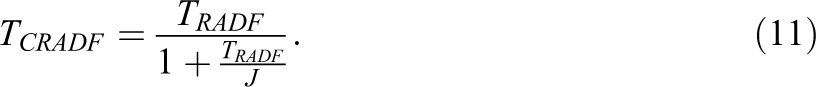
The residual-based test statistics TRADF and TCRADF
Browne (1982, 1984) described a class of residual-based test statistics based on arbitrary distributional assumptions. A thorough discussion of these statistics can be found in Foldnes et al. (2012). Yuan and Bentler (2007) adapt Browne’s (1984) residual-based asymptotically distribution-free statistic for use in conjunction with the segregating method. The residual-based test statistic, T RADF, is given by
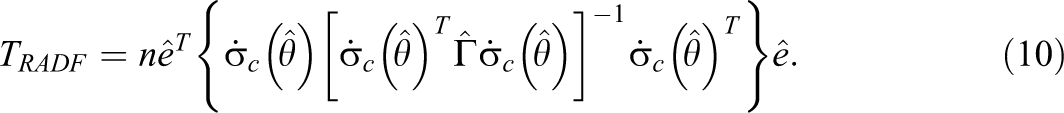
In conventional factor analysis,
Yuan and Bentler (1998, 2007) suggested a small sample corrected version to T RADF for use in conjunction with the segregating method:
Neither TRADF
nor TCRADF
will be defined unless
The rescaled test statistic TRML
TRML was designed to rescale TML based on excess skew and kurtosis in the observed variables (Satorra & Bentler, 1988). Let

Also let

Yuan and Bentler (2007) proposed a version of TRML
for use in conjunction with the segregating method, where WML
= WB
, the weight matrix in Equation 9 evaluated at Σ
B
(θ),
Behavior of TML in the Segregating Methodology
In using the segregating method, TML is often expected to converge to a central χ2 distribution with d degrees of freedom if the model is correct and there is no excess skew or kurtosis in the observed variables. Several sources (Goldstein, 2003; Hox, 2010; Hox & Maas, 2004; Ryu & West, 2009) suggested that TML will behave in this way and can be used to evaluate the between-level measurement models.
In practice, however, and contrary to the advice given in these sources, TML may be inflated and may not have the correct asymptotic distribution, even when the data are normally distributed and the model is correctly specified. The extent of the inflation will be related to (1) the proportion of total observed variance attributable to group membership (i.e., the intraclass correlations [ICCs] of the observed variables) and (2) within-group sample size.
For clarity of presentation, we will assume that the groups are balanced (i.e., m 1 = m 2 = … = mj = m) and that the observed scores (as defined in Equation 1) are multivariate normal in distribution. The ICC represents the proportion of observed variance attributable to group membership and can be obtained from the diagonal elements of Σ B and Σ W . For any given item p, the ICC can be expressed:
where Σ
Bpp
and Σ
Wpp
are the diagonal elements of Σ
B
and Σ
W
, respectively. ICC values range between 0 and 1, and for a fixed value of
Under normal theory, the asymptotic covariance matrix of
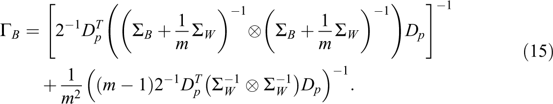
Γ B depends not only on information from Σ B but on information from Σ W as well.
When a factor analysis is performed on
The ignorability of these terms is directly related to the ICC of the observed variables and within-group sample size. Keeping Σ B fixed, as the ICC increases, Σ W approaches zero, and the terms involving Σ W in Equation 15 become ignorable. For low ICCs, where Σ W is relatively large, these terms will not be ignorable. Alternatively, keeping ICC fixed, as m, the within-group sample size, increases, the terms involving Σ W in Equation 15 become ignorable. For small within-group sample sizes, these terms will not be ignorable.
This implies that FML
is particularly likely to be misspecified for WB
when ICCs are low or within-group sample sizes are small. Under those conditions, TML
will not converge in distribution to a centrally distributed χ2 variate, even when the model is correct and the number of groups is sufficiently large. As a result, inferences about model structure based on TML
may not be valid for the segregated analysis of
Behavior of the Residual-Based Test Statistics
Unlike TML
, the residual-based and rescaled test statistics use information from both between and within covariance sources through
TRML
is expected to converge to a distribution with the correct first moment regardless of ICC and within-group sample size. The scaling constant, k, will be greater than 1. In conventional, single-level factor analysis, Bentler (2006) explained that
Issues With TML in the Study of Classroom Climate
The relationship between the discrepancy function, the weight matrix, item ICCs, and within-group sample size is rarely made explicit in the methodological literature on multilevel factor analysis. Even when the poor performance of TML is noted (Muthén, 1994, p. 389; Hox, 2010; Yuan & Bentler, 2007), the possible role of either item ICC or within-group sample size in the misspecification of F ML for WB is not described. In fact, several sources (Goldstein, 2003; Hox, 2010; Hox & Maas, 2004; Ryu & West, 2009) suggested that the segregating method is a “viable method” (Hox & Maas, 2004, p. 145) that can be “implemented within the preexisting ML SEM framework” (Ryu & West, 2009, p. 600).
As a result, there is confusion in the applied literature on the interpretation of TML . There are many cases in the applied literature where an inflated valued of TML is interpreted as suggesting model misspecification and often the theorized between-group model is then modified by removing items, adding additional factors, or modifying paths (e.g., Mathisen et al., 2006). The possibility that TML may also reflect the fact that FML is misspecified for WB is unexplored and untested.
The advice to use TML for model fit assessment is particularly problematic when the segregating method is used to assess the factor structure of classroom climate surveys, because the two conditions most likely to cause issues with the performance of TML —low item ICCs and relatively small within-group sample sizes—are particularly common in this field. Generally speaking, item ICCs for climate variables are “often less than .1 and rarely greater than .3” (den Brok, Bergen, Stahl, & Brekelmans, 2004; Marsh et al., 2012, p. 115; Toland & De Ayala, 2005). Class sizes typically range between 12 and 25 students per class (e.g., Holfve-Sabel & Gustaffson, 2005; Kunter et al., 2008). Under these conditions, the inflation of TML is likely to be severe. Relatedly, Type I error rates are likely to be far higher. It is unlikely that inferences about the between-classroom measurement models based on TML would be valid.
Because TML is expected to perform poorly in the evaluation of between-level measurement models for classroom climate surveys, it may seem reasonable to recommend the use of alternative test statistics, such as the residual-based and rescaled test statistics, since the theory outlined previously suggests these statistics should perform well asymptotically. In fact, Yuan and Bentler (2007) recommended the use of TRML and TCRADF for model evaluation in conjunction with the segregating method. However, there is only limited simulation work with the residual-based and rescaled test statistics in a multilevel context, and there are many known issues with statistics like TRADF , TCRADF , and TRML in conventional factor analysis, particularly with small sample sizes and large models, which may be expected to present problems in multilevel investigations (e.g., Bentler & Yuan, 1999; Curran, West, & Finch, 1996; Hu, Bentler, & Kano, 1992; Muthén & Kaplan, 1985, 1992; Powell & Schaefer, 2001; Yuan & Bentler, 1998). In conventional factor analysis, when models are large and sample sizes are small, TRADF and TRML tend to overreject correct models, and TCRADF tends to underreject correct models (Yuan & Bentler, 1999).
In fact, as it turns out, these specific conditions (small sample sizes and large models) are also likely to occur with student surveys of classroom climate. In the literature on student surveys of classroom climate, the number of classrooms (i.e., the group-level sample size) is typically between 50 and 500 (e.g., Fauth, Decristan, Riser, Klieme, & Buttner, 2014; Holfve-Sabel & Gustaffson, 2005; Kunter et al., 2008; Toland & De Ayala, 2005). Measurement models range from 25 degrees of freedom to well over 150 degrees of freedom (e.g., den Brok et al., 2004; Fauth et al., 2014; Holfve-Sabel & Gustaffson, 2005; Kunter et al., 2008; Toland & De Ayala, 2005).
It is not clear whether, under these conditions, the residual-based test statistics or the rescaled test statistics would continue to perform well. It is also unclear whether Yuan and Bentler’s (2007) recommendations to use TRML and TCRADF , which were based on a simulation study using high item ICCs, large within-group sample sizes, relatively small measurement models, and a large number of groups, would be supported under a wider range of conditions, particularly those typically found in survey-based research on classroom climate.
This study uses an illustrative example and a simulation in order to (a) illustrate the extent to which the ML test statistic will be inflated, (b) demonstrate how item ICC and within-group sample size influence the distribution of TML
, (c) investigate the performance of several alternative test statistics—specifically TRML
, TRADF
, and TCRADF
—under a broader range of conditions, particularly those that are frequently encountered in survey-based research on classroom climate. The empirical example comes from the Tripod Classroom Environment Survey (Ferguson, 2010), which is administered to measure aspects of classroom environment. Using the illustrative example and the simulation study, the following four research questions were addressed:
Method
Data Sources
The Tripod Classroom Environment Survey
The Tripod Survey (Ferguson, 2010) is designed to assess seven dimensions of teaching practice, often referred to as the “Seven Cs”: caring, captivating, conferring, clarifying, challenging, controlling, and consolidating. This version of the Tripod Survey was administered in an urban school district in California in 2010. This example uses 5 items from the “challenging” dimension that are rated on 5-point scales (1 = totally untrue and 5 = totally true). The sample used in this analysis contained 5,508 students in 285 classrooms. The average classroom size was approximately 17 students. Students are treated as nested within classrooms, and it is assumed that each student has rated only one classroom. Descriptive information about the survey items is summarized in Table 1.
Descriptive Statistics for Tripod Survey Variables
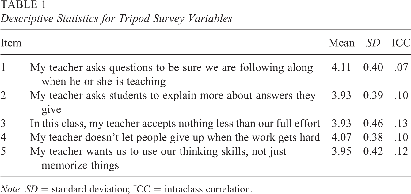
Note. SD = standard deviation; ICC = intraclass correlation.
Simulated data sets
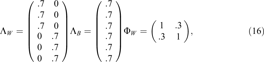
Data were generated from multivariate normal distributions and a population model with two within-level factors and one between-level factor. This population model was selected because several sources suggest that the between-level factor structure is likely to be simpler than the structure at the within level (e.g., Holfve-Sabel & Gustaffson, 2005; Muthén & Asparouhov, 2011). Simulation conditions were selected in order to reflect the conditions commonly reported in survey-based research on classroom climate. The following four conditions were manipulated: (1) item ICCs (ICC = .50, ICC = .26, ICC = .10, and ICC = .05), (2) Level 2 sample size (J = 100, J = 200, and J = 500), (3) group size (n = 10, n = 30, and n = 50), and (4) the size of the measurement model (df = 9, df = 54, and df = 135).
For the ICC = .5 condition with six observed variables, the generating model used the following parameters:
Analytic Approach
To address the first research question, the Tripod Survey data were used. ML estimates of Σ
B
and Σ
W
were obtained. 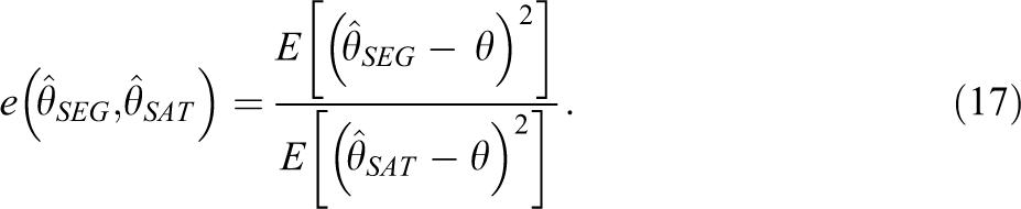
If
Simulated data were also used to answer the third research question. For each simulation condition, the mean and standard deviation of TML
were estimated, and an empirical Type I error rate was calculated. For the purpose of this study, the Type I error rate was calculated at the nominal α = .05 level. Because it is expected that the empirical error rates will differ somewhat from the nominal rate, an acceptable empirical error rate is taken as one that falls in the interval [.028, .079], the estimated two-sided 99% adjusted Wald confidence interval (e.g., Agresti & Coull, 1998). In addition to TML
,
In order to address the fourth research question, investigating the performance of TRML
, TRADF
, and TCRADF
under a range of conditions similar to those encountered in survey-based research on classroom climate, means and standard deviations of these three test statistics were estimated for each simulation condition, and an empirical model rejection rate was calculated. As in the case of TML
, the rejection rate was calculated at the nominal α = .05 level and acceptable rates were those in the interval [.028, .079]. It should be noted that for several conditions (when J = 100 and df = 135), the residual-based test statistics are not estimable because
Results
To What Extent Can Inferences About the Measurement Structure of the Tripod Classroom Environment Survey Based on TML Differ From Those Based on Residual-Based and Rescaled Test Statistics?
The estimate of TML
is 136.9. This can be referred to as
However, based on the theoretical results presented previously, there is reason to suspect that the TML test statistic should not be trusted in this particular case. First, the item ICCs are fairly low, ranging from .07 to .13 (Table 1). Second, the average number of individuals in each classroom is fairly small. Even if all of the distributional assumptions were satisfied, with ICCs that are in this range, the correct specification of FML for WB would require much larger classroom sizes in order for TML to have the correct distribution. Thus, it may be more appropriate to make model inferences based on rescaled or residual-based test statistics. Here, TRADF (4.54, p = .454), TCRADF (4.47, p = .484), and TRML (5.50, p = .358) all suggest strong evidence for failing to reject the null hypothesis. In other words, these three test statistics all suggest that the items are indeed unidimensional, an inference that completely contradicts the inference based on TML .
It should be noted that while this example provides a clear illustration of how low ICCs and small within-group sample sizes can distort inferences about the between-classroom model based on TML , it was also limited in some important ways. First, the data-generating mechanism was unknown. While the inflation of TML relative to TRADF , TCRADF , and TRML is related to ICC and within-group sample size, it is possible that other factors, including multivariate kurtosis, play a role in model appraisal. Second, the model is relatively small, containing only five variables and 5 degrees of freedom, and so while the rescaled and residual-based test statistics provide valid inferences in this case, these results may not generalize to larger models. These issues are addressed in the analyses that follow.
Is There a Loss of Estimator Efficiency in Using the Segregating Method, as Compared to the Partially Saturated Model Method?
Table 2 displays the relative efficiency of parameter estimation under both the segregating method and the partially saturated model method across all simulation conditions. Table 2 displays results for only one model size condition (df = 9), but the results are consistent across all model sizes. These results suggest that there is, in general, no loss of efficiency that comes from using the segregating method. Supporting the hypotheses of Yuan and Bentler (2007), there is even a slight gain in efficiency for the segregating method as the ICCs get smaller and the group sizes get smaller. At ICC = .05 with a small number of groups and only 10 individuals in each group, the segregating method is far more efficient than the partially saturated model method. Although not evident from Table 2, it should be noted that while the segregating method is relatively more efficient in the condition with ICC = .05, n = 10, and J = 100, there is considerably more variability in the parameter estimates overall, perhaps reflecting some numerical instability.
Efficiency of the Segregating Method Relative to the Partially Saturated Model Method
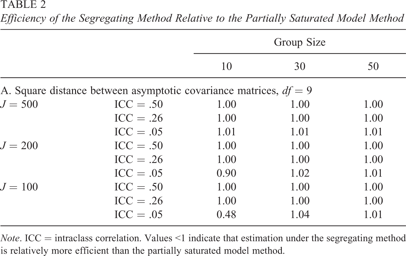
Note. ICC = intraclass correlation. Values <1 indicate that estimation under the segregating method is relatively more efficient than the partially saturated model method.
How Do Item ICC and Within-Group Sample Size Influence the Distribution of TML
? How do Item ICC and Within-Group Sample Size Influence the Differences Between
and
?
Tables 3 present the test statistic means, variances, and empirical Type I error rates across a selected subset of simulation conditions. For compactness of presentation, results for ICC =.10 are not displayed but are consistent with the results displayed here. As expected, as either ICC or within-group sample size decreases, TML increases and, relatedly, Type I error rates increase. TML is only well behaved with 500 groups, more than 30 individuals per group and an ICC of .50 (Table 3, Panel A). This condition is most similar to the simulation conditions of Ryu and West (2009) and Hox and Maas (2004) and offers some insight into why those studies concluded that ML methods and the likelihood ratio test statistic were appropriate for use in conjunction with the segregating method.
Test Statistic Means, Standard Deviations, and Type I Error Rates for TML
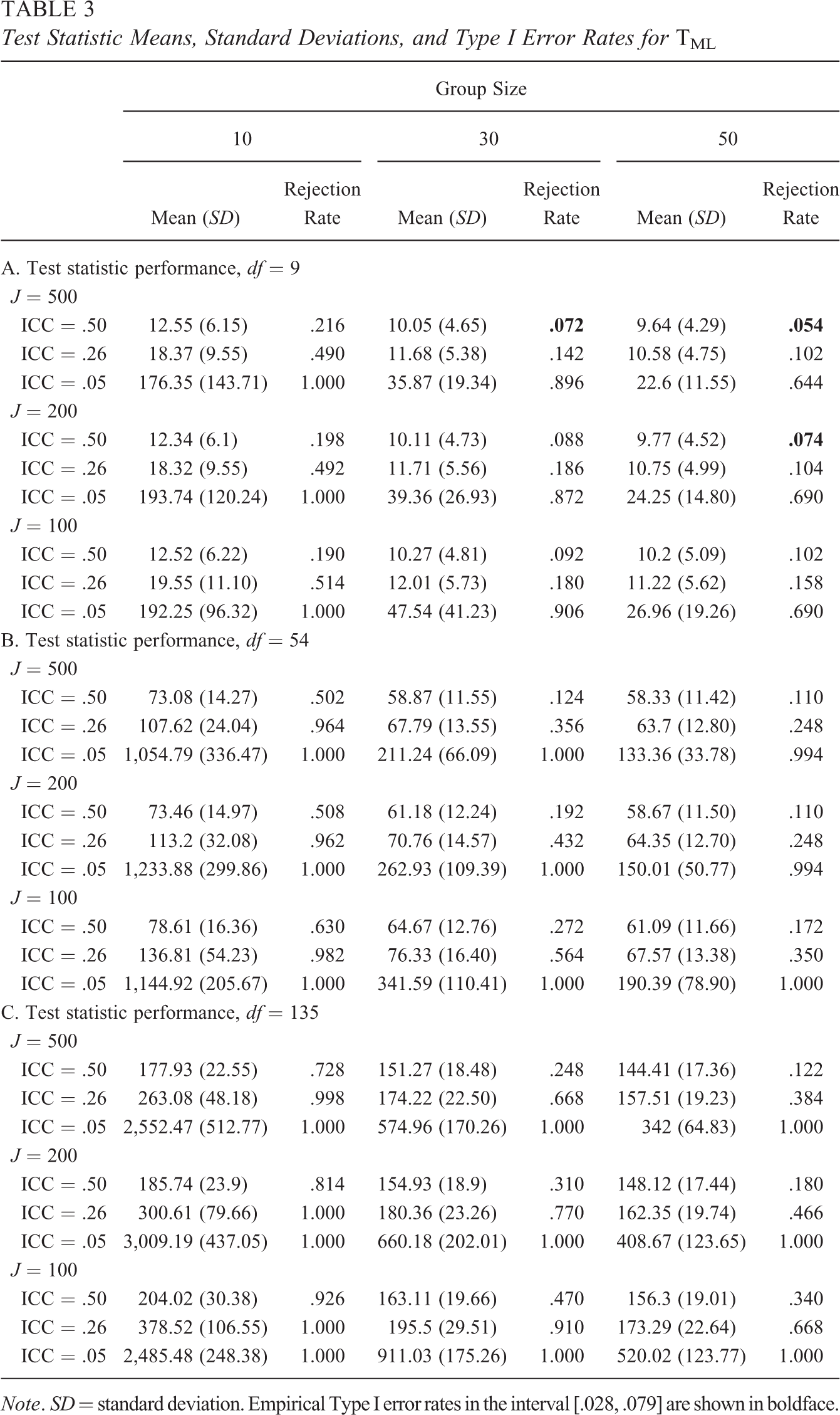
Note. SD = standard deviation. Empirical Type I error rates in the interval [.028, .079] are shown in boldface.
TML inflation can be quite severe. When ICCs are low and the within-group sample sizes are small, the correct model is rejected 100% of the time, and the test statistic mean is about 20 times larger than expected, for all model sizes. This pattern of inflation suggests that TML will not provide valid inferences about between-classroom measurement models in survey-based research on classroom climate. The results presented in Table 3 also suggest little evidence that TML would ever converge to the correct distribution, regardless of the number of groups that are included in the sample. For example, for ICC = .50, with within-group sample sizes of 10, there is little evidence of convergence as the number of groups increases from 100 to 500.
Table 4 presents the distances between
Squared Distances Between Asymptotic Covariance Matrices
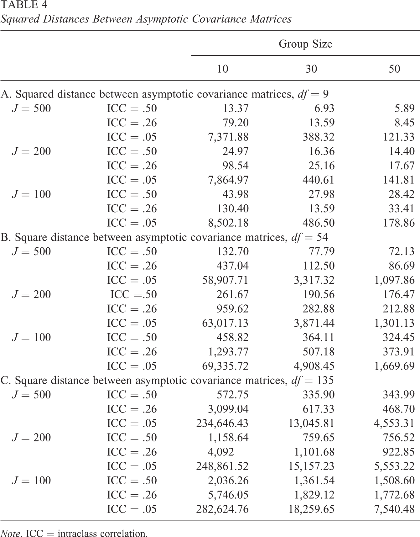
Note. ICC = intraclass correlation.
How do TRML , TRADF , and TCRADF Perform Under a Broader Range of Conditions, Particularly Those That Are Frequently Encountered in Survey-Based Research on Classroom Climate?
Performance of TRADF
Consistent with theoretical expectation, there is evidence that TRADF converges to the correct distribution as the number of groups increases regardless of ICC or within-group sample size. This pattern of convergence is most apparent in Table 5 (Panel A), as the number of groups increases from 100 to 500. With 100 groups, TRADF overrejects the correct model for nearly all ICC and within-group sample size conditions. Contrary to this pattern, TRADF has a mean that is too low at ICC = .05 and n = 10, which may reflect some of the instability of the estimates at low ICCs and small sample sizes. With 500 groups, TRADF is much better behaved. However, when the model is sufficiently large, the number of groups would have to be enormous in order for TRADF to provide correct inferences. In Table 5 (Panel C), when the model is large and the number of groups is small, TRADF rejects the correct model 100% of the time. Even with 500 groups, the empirical Type I error rates approach 90%. This is consistent with results from both conventional and multilevel factor analysis, where it has been shown that TRADF and other similar statistics converge slowly to the appropriate distribution (e.g., Curran et al., 1996; Hu et al., 1992; Muthén & Kaplan, 1985, 1992; Powell & Schaefer, 2001; Yuan & Bentler, 1998, 2003, 2007).
Test Statistic Means, Standard Deviations, and Type I Error Rates for TRML , TRADF , and TCRADF
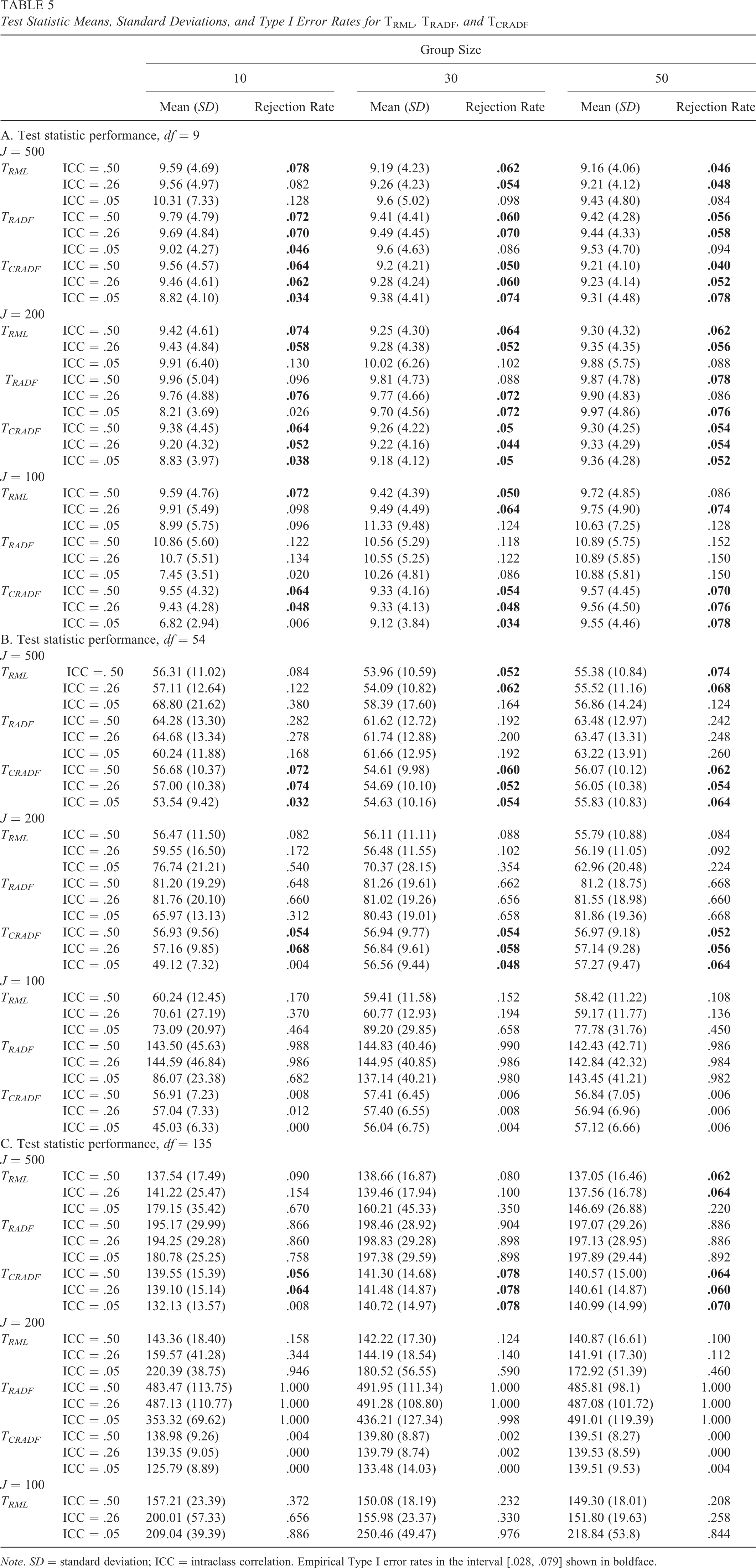
Note. SD = standard deviation; ICC = intraclass correlation. Empirical Type I error rates in the interval [.028, .079] shown in boldface.
Performance of TCRADF
TCRADF shows well-behaved means, standard deviations, and empirical Type I error rates across a wide variety of simulation conditions. Table 5 (Panel A), which displays results for the small models (df = 9), shows that TCRADF performs well when the number of groups is sufficiently large, relative to the size of the model. This pattern continues in Table 5 (Panel B), with the medium-sized models (df = 54), provided that the number of groups is sufficiently large (J = 200 or J = 500). However, when the number of groups is small relative to the size of the model (e.g., in the condition with J = 100 and df = 54), the multilevel version of TCRADF performs similarly to the conventional version (Bentler & Yuan, 1999; Yuan & Bentler, 1998). That is, the statistic accepts more correct models than would be expected by chance.
Performance of TRML
Consistent with theory, in all ICC and group size conditions, the scaling constant for TRML
, k, is larger than 1. The amount of rescaling changes as a function of within-group sample size and item ICC. At ICC .50, there is virtually no rescaling at all. At ICC .05, the TML
value is scaled by almost 90%. There is also some evidence that the mean of TRML
converges appropriately as the group number increases. For small models, relatively large sample sizes and high ICCs, TRML
behaves well. These conditions are most similar to the conditions that lead Yuan and Bentler (2007) to recommend TRML
for model testing. However, when the full range of simulation conditions are considered, it becomes clear that TRML
cannot adequately control Type I errors when group sizes are small or when ICCs are low. In the condition where
Summary and Conclusion
As surveys of the classroom environment have gained traction as components of teacher evaluation portfolios, there has been an increased amount of attention paid to using multilevel factor analyses to explore hypotheses about the measurement structure of between-classroom phenomena. The segregating method has many theoretical benefits. It allows for the separate testing and identification of measurement models at the between level and within level. This is a key advantage over approaches that simultaneously fit models to Σ B and Σ W , since many studies have found that the simultaneous testing of between and within models can make diagnosing sources of model misfit difficult (e.g., Hox, 2010; Ryu & West, 2009; Yuan & Bentler, 2007).
The current study, however, clarifies an important characteristic of the segregating method for applied research. Namely, at ICC and sample size configurations likely to be encountered when data about the classroom environment are collected by surveying students, the commonly used ML test statistic obtained from the segregating method is likely not asymptotically distributed as central χ2 variates under the null hypothesis. This suggests that the reliance on the ML test statistic can result in unwarranted model modifications or revisions.
The current study used an illustrative example and a simulation study to investigate the performance of test statistics under conditions likely to be encountered in using the segregating method in applied research on classroom climate. The results reflect some general patterns that are worth noting here. As with any simulation study, caution should be used in generalizing these results to other conditions not included in the study. More work would be needed to investigate how other conditions, such as differences in factor loadings, alternative (nonnormal) distributions, and imbalanced group-sizes, would influence the performance of test statistic.
Estimation Under the Segregating Method Can Be as Efficient as the Partially Saturated Model Method
While it is often assumed that because the segregating method requires two separate steps for implementation, there will be a loss of efficiency as compared to single-step approaches such as the partially saturated model method, and the results of this study suggest that the segregating method can be as efficient as the partially saturated model method, and under certain conditions—with small sample sizes, low ICCs and large models—the segregating method can be considerably more efficient. Goldstein (2003) suggested that the segregating method may lose efficiency if the group sizes are highly unbalanced, a condition which is beyond the scope of the current investigation. Further research would be needed to investigate the joint influence of group size imbalance, ICC, and model size on efficiency.
Inferences About Model Fit Based on T ML Can Lead to Invalid Conclusions About the Between-Classroom Factor Structure
At ICC and sample size configurations likely to be encountered when data about classroom climate are collected by surveying students, TML
is not asymptotically distributed as central χ2 variate under the null hypothesis. The Tripod Survey example demonstrated that inferences based on TML
can lead to invalid conclusions about the between-classroom factor structure when ICCs are low and within-classroom sample sizes are small. The simulation study shows the extent to which TML
can be inflated. The simulation results show that in some conditions, the mean of the test statistic was nearly 20 times too large, and every model was rejected. Thus, TML
behaved very poor in general and should not be used to make inferences about the between-level measurement models. While beyond the scope of the current study, these results suggest that, beyond issues with assessing model fit, ML estimation would result in biased standard errors. This is because, typically speaking, estimated standard errors are computed using
TCRADF Can Provide Valid Inferences, Provided the Number of Groups Is Sufficiently Large
While both the rescaled and residual-based test statistics show evidence supporting the hypothesis that they would converge to the appropriate distribution regardless of item ICC and within-group sample size, only TCRADF showed adequate performance over a wide range of conditions. TRADF showed a tendency to overreject correct models for all but the largest samples, consistent with findings in conventional factor analysis. TRML , too, overrejected correct models, particularly for small between-level sample sizes. Only TCRADF is recommended for use in conjunction with the segregating methodology. However, caution should be used with small samples, where TCRADF shows a tendency to underreject correct models.
Footnotes
Acknowledgments
The author is grateful to Joan Herman, Jia Wang, and Noelle Griffin for their support and to Peter Bentler, Li Cai, and Jose Felipe Martinez for their valuable advice and feedback.
Author’s Note
The findings and opinions expressed in this report are those of the author and do not necessarily reflect the positions or policies of the Bill and Melinda Gates Foundation or the U.S. Department of Education.
Declaration of Conflicting Interests
The author(s) declared no potential conflicts of interest with respect to the research, authorship, and/or publication of this article.
Funding
The author(s) disclosed receipt of the following financial support for the research, authorship, and/or publication of this article: The research for this article was supported in part by grant number 52306 from the Bill and Melinda Gates Foundation with funding to the National Center for Research on Evaluation, Standards, and Student Testing (CRESST). Part of this research was made possible by a predoctoral advanced quantitative methodology training grant (#R305B080016) awarded to UCLA by the Institute of Education Sciences of the U.S. Department of Education.