How Generalizable Is Your Experiment? An Index for Comparing Experimental Samples and Populations

Abstract

Although a large-scale experiment can provide an estimate of the average causal impact for a program, the sample of sites included in the experiment is often not drawn randomly from the inference population of interest. In this article, we provide a generalizability index that can be used to assess the degree of similarity between the sample of units in an experiment and one or more inference populations on a set of selected covariates. The index takes values between 0 and 1 and indicates both when a sample is like a miniature of the population and how well reweighting methods may perform when differences exist. Results of simulation studies are provided that develop rules of thumb for interpretation as well as an example.

Keywords

generalizability external validity experiment causal inference index

In the educational and social sciences, experiments are prized for their high degree of internal validity. The random assignment of treatment conditions within the experiment ensures that the treatment effect estimated is causal. A problem not addressed by this random assignment, however, is how to generalize the findings from the units in the experiment to a larger inference population. The statistical ideal for this causal generalization requires two steps. First, the experimental sample is randomly selected from a well-defined inference population, and second, units in the experimental sample are assigned randomly to treatment conditions. Unfortunately, this dual randomization procedure is exceedingly rare in practice; for example, Olsen, Orr, Bell, and Stuart (2013) found that random site selection was implemented in only 7 of 273 experiments in the Digest of Social Experiments (Greenburg & Schroder, 2004). The fact that random sampling is so rarely used means that in contrast to the statistically sophisticated methods used for dealing with threats to internal validity (e.g., attrition), the methods used for generalizing from the experiment to policy-relevant populations are typically a-statistical and not well defined (Cornfield & Tukey, 1956).

Recent research has begun to formalize and address this causal generalization problem. By comparing experimental impact estimates of the Reading First program with changes in school test scores after multiple states adopted the curricula, Stuart, Olsen, Bell, and Orr (2012) showed that external validity bias can be as large as the internal validity bias that occurs in observational studies (in which treatment is not assigned randomly). The fact that the generalization problem has many similarities to the observational studies problem led Hedges and O’Muircheartaigh (2011) to propose to use post-stratification methods with population information to reweight units in the experiment so that the experimental sample is compositionally similar to the inference population. This idea is similar to standardization in demography (Kitagawa, 1964) and employs propensity score methods (Rosenbaum & Rubin, 1983). Tipton (2013) studied the assumptions needed for this post-stratification approach and showed what effects in terms of bias and variance inflation could be expected in practice. Similarly, Bareinboim and Pearl (2013) investigated the assumptions necessary for generalizability—what they call “transportability”—using a graph theoretic approach. Finally, the fact that any post hoc adjustment aimed at generalization is likely to increase the sampling variance in the treatment impact estimate led Tipton et al. (2014) and Tipton (2014) to propose new methods for site selection aimed at improving generalizations through design.

Like Stuart, Cole, Bradshaw, and Leaf (2011), this article focuses instead on methods for assessing the generalizability of an experimental sample for a particular inference population. The index we propose does not focus on a particular outcome measure or treatment effect estimator. The goal is to develop a generalizability index based only on pretreatment covariates that allow for easy and meaningful comparisons between an experimental sample and population. Unlike Stuart et al. (2011), the generalizability index we propose is bounded: It takes values in [0,1], with 1 indicating that the experimental sample is “representative” of the population and a 0 indicating that the experimental sample and population do not overlap at all. The index we propose is based on the Bhattacharyya coefficient (1943, 1946), which is widely used in pattern recognition, genomics, and ecology and could be of use not only in generalization but also in assessing balance in observational studies. By focusing only on pretreatment covariates, this index allows the generalizability issues to be isolated and separated from other design and analysis choices, making it useful both retrospectively and as a tool during study design.

This article is organized as follows. We begin by reviewing the recent literature using propensity scores for generalization, including current metrics for comparing samples and populations. We then introduce a new generalizability index and, after investigating theoretical properties of this index, report results of simulation studies aimed at developing rules of thumb. We then provide an example comparing the composition of schools in an experiment to the compositions of schools in different states. We conclude with a discussion of other possible uses.

Using Propensity Scores for Generalization

Overview

In this section, we review the generalization framework developed by Stuart et al. (2011), Hedges and O’Muircheartaigh (2011), and Tipton (2013). We begin by assuming that we have an experimental sample S that contains n units, and an inference population P that contains N units. Throughout this article, we use the term units, which could be individuals or their aggregates. In experimental generalization, the units are typically defined at the level of sampling, which occurs at the level of treatment assignment or higher; in large-scale educational experiments, the units might be schools or school districts, while in other studies they might be sites or clinics. For each unit in the population and experimental sample, let W = 1 indicate whether a unit receives the treatment condition and W = 0 otherwise. Then for a particular outcome Y, let Y(0) = Y(W = 0) be the potential outcome for a unit under the control condition and Y(1) = Y(W = 1) be the potential outcome for the unit under the treatment condition (Rubin, 1974). The unit’s treatment effect is defined as Δ = Y(1) – Y(0). In causal generalization, the goal is typically to estimate the population average treatment effect (PATE), E _p(Δ), where E _p(.) is the average value of Δ for all units in the population P.

Definition: Sampling propensity score

Let Z = 1 if a unit is in the experimental sample S (vs. the population P), and X = (X ₁, X ₂,…, X _m) be a set of covariates. This set of covariates can include both continuous measures and categorical variables, and we do not require any distributional assumptions. The sampling propensity score is defined as:

s (X) = P r (Z = 1 | X) .

The propensity score is a balancing score, which means that for each value of s(X), the distribution of X is the same in the experimental sample and population (Rosenbaum & Rubin, 1983). Although the sampling propensity score is a theoretical quantity, it can be estimated using a simple logistic regression model,

l o g [s (X) / (1 - s (X))] = α_{0} + α_{1} X_{1} + . . . + α_{m} X_{m} .

These estimated propensities (or their logits) are used to get a better estimator of PATE (Rubin & Thomas, 1996). Propensity scores reduce the problem from matching on a multivariate X to matching on a univariate s(X) while also not requiring any distributional assumptions on the underlying covariates in X. An important question in generalization is which covariates should be included.

Assumption: Unconfounded sample selection

The sampling process and the unit treatment effects are conditionally independent, given the propensity score s(X),

Δ = [Y (1) - Y (0)] ⊥ Z | s (X) .

This assumption means that X must include all covariates that both explain variation in the treatment effects and differ in distribution in the population P and experimental sample S. A difficulty with this assumption is that it is rarely possible to test directly, particularly given both the small sample sizes that are typical (n ≤ 60) and the fact that in cluster-randomized studies, site-specific treatment impacts cannot be identified. For these reasons we suggest that the covariates in X are selected based on prior empirical evidence and theoretical considerations; Rubin (2001) makes a similar recommendation when using propensity scores in quasi-experiments.

Proposition: Strongly ignorable sample selection

The experimental sample is said to be strongly ignorable, given the sampling propensity score if

Δ = [Y (1) - Y (0)] ⊥ Z | s (X) a n d 0 < s (X) \leq 1.

In finite samples, strong ignorability requires that, in addition to meeting the unconfounded sample selection assumption, the distribution of X in the population P and experimental sample S share common support. This condition can fail for one of two reasons. One reason is if there are no units in the experimental sample similar to some units in the population. Tipton (2013) refers to this problem as a coverage error, akin to the type of error that arises in survey sampling when the target population and population frame do not align exactly (see Groves, Fowler, Couper, Lepkowski, & Singer, 2009). This problem can be summarized by saying that the proportion

θ = N_{0} / N \leq 1

of the population is represented in the experiment, where N ₀ is the number of population units in the common support region and N is the total population size. Statistically, this means that in order to generalize to the full population, extrapolations will be required.

The second way that the common support condition can fail is if there are units in the experimental sample with no similar population units. This problem arises if, for example, the experiment was conducted on a set of urban and rural schools, but PATE is desired for a county that only includes urban schools. This problem can be summarized by saying that the proportion

φ = n_{0} / n \leq 1

of the experimental sample is represented in the population, where n ₀ is the number of experimental sample units in the common support region and n is the total sample size in the experiment. This means that only 100φ% of the experimental sample is relevant for estimating PATE, or, put another way, 100(1 − φ)% of the units are not needed. This has clear implications for statistical efficiency and power, since discarding sample units both reduces bias and the total sample size used to estimate the average treatment effect.

Estimators, Bias, and Sampling Variance

After defining the propensity score and determining the common support region, PATE can be estimated using a variety of propensity score estimators. Hedges and O’Muircheartaigh (2011), Tipton (2013), and O’Muircheartaigh and Hedges (2014) focus on the use of the propensity score subclassification estimator. All propensity score–based estimators are similar in that they use the distribution of propensity scores in the population P to in some way reweight the units in the experimental sample S so as to adjust for compositional differences in X. These estimators are in contrast to the simple difference in means estimator (the naive estimator) typically used in experiments or its more complicated analogue when the data are multilevel (Raudenbush & Bryk, 2002).

Tipton (2013) evaluated the effectiveness of the subclassification estimator in terms of bias reduction and variance inflation, as compared to the naive estimator. She found that the degree of bias reduction and variance inflation was a function of three quantities, that is, θ, φ, and the degree of distributional similarity within the common support region. In general, Tipton shows that there are several trends: As θ decreases so too does the maximum possible bias reduction; as φ decreases, the sampling variance increases; and as the degree of distributional similarity decreases, both maximum bias reduction and variance inflation increase. It is the goal of this article, therefore, to develop a generalizability index that takes into account all three of these factors, indicating when an experimental sample is likely to contain enough information for PATE estimate to be calculated that is useful, where by useful we mean both precise and close to unbiased.

A Generalizability Index

The Standardized Mean Difference

The goal of this article is to develop an index that takes into account the three quantities introduced earlier that affect the bias and sampling variance of a reweighted estimator of PATE. As we have framed the problem, the assessment of generalizability should focus not only on the similarity between the experimental sample and population but also on how effective propensity score adjustment methods may be in creating a useful estimate of PATE. In doing so, the index distinguishes between situations in which baseline bias can be successfully removed and those in which the differences cannot be removed.

The idea of quantifying the degree of similarity between the experimental sample and population as a method for assessing the degree of generalizability was first proposed by Stuart et al. (2011). They proposed that, like in quasi-experiments, the standardized mean difference (SMD; δ) between the propensity score distributions in the experimental sample and population could be used as such a metric, where

δ = (μ_{s} - μ_{p}) / σ,

and where μ _s and μ _p are estimated by the means of the estimated propensity scores (or their logits) in the sample and population, respectively, and σ² is estimated either using the population variance estimate (s_p ²) or using a pooled estimate of the variance in the experimental sample and population, s ² = {(n – 1) s_s ² + (N – 1)s_p ²}/(N + n − 2), where s_s ² is the estimated variance of the propensity score distribution (or logits) in the experimental sample.¹ They illustrate this with an example in which δ is estimated to be .73 when comparing the sample of schools in the Positive Behavioral Interventions and Support study to a population of schools in Maryland. By applying the rules of thumb commonly used in quasi-experiments (e.g., |δ| < .25), they argue that this is a large difference, and by bootstrapping, they show that it would occur by chance in less than 1% of randomized samples.

Although the SMD is a natural summary statistic for assessing the degree of similarity between two distributions (particularly two normal distributions), it does not capture well the potential effectiveness of a reweighting estimator aimed at estimating PATE. In order to see why, in Figure 1 we illustrate six possible distributional comparisons using two plots. In each plot, three possible population distributions are compared to a sample distribution. In the plot on the left, the distributions compared are both normally distributed, while on the right-hand side, beta distributions are compared. This approximates the distributions of propensity scores (right) and their logits (left). In all six comparisons, the SMD between each of these populations and the sample is .75, although as is immediately clear, the degree of overlap and distributional similarity varies widely. For example, in both plots, the comparison between the sample and “Population 3” clearly results in larger overlap problems (θ < 1, φ < 1) than does that between the sample and “Population 1.” As results from Tipton (2013) and additional simulations indicate (presented later in this article), the degree of bias reduction and cost in terms of variance inflation when using the reweighting approach is therefore higher for Population 3 than for Population 1.

Figure 1.

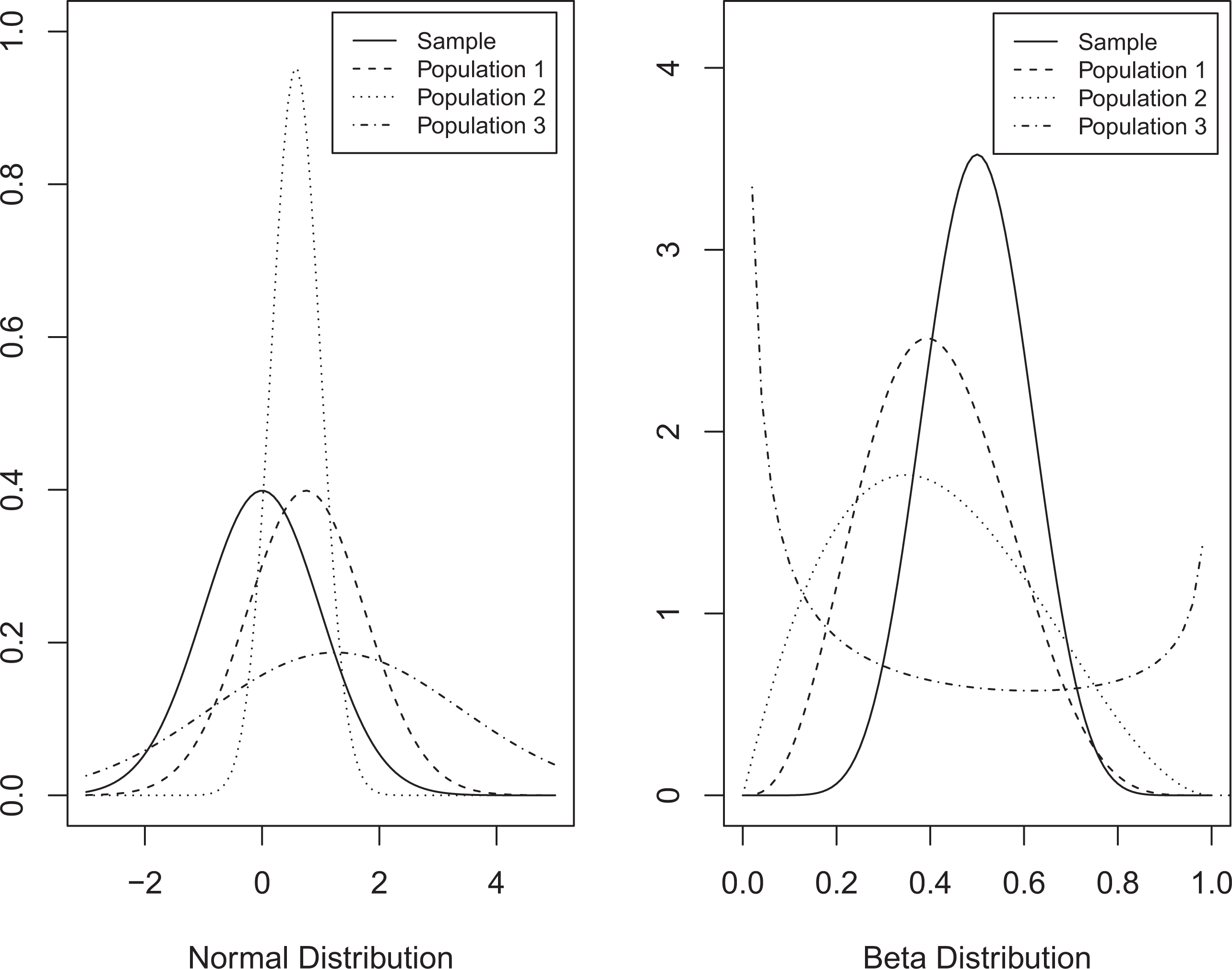
Six density comparisons with |SMD| = 0.75. SMD = standardized mean difference.

Although Stuart et al. (2011) focus on the SMD (as well as the unstandardized difference in probabilities), in the quasi-experimental literature other methods are also recommended for assessing the degree of similarity (“balance”) between two propensity score distributions (Ho, Imai, King, & Stuart, 2007). One of the most common methods is to visually compare the distributions using empirical density plots, histograms, and jitter plots (Stuart, 2010). In addition to the SMD (δ), these observed differences in the densities are often supplemented with the ratio of variances, which in generalization would be defined as

ω^{2} = σ_{s}^{2} / σ_{p}^{2},

where σ _s ² and σ _p ² are the variances in the propensity score distributions (or their logits) in the experimental sample and population, respectively.

More recently, other measures of distributional balance have been proposed. These include visual methods like Q–Q plots (Ho et al., 2007) as well as the Kolmogorov–Smirnov distance, Levy distance, and the overlapping coefficient (Belitser et al., 2011) as well as the C statistic (Franklin, Rassen, Ackermann, Bartels, & Schneeweiss, 2014). Interestingly, although the most common visual method for comparing the propensity score distributions focuses on densities (e.g., histograms, empirical densities, jitter plots), nearly all of these distributional balance statistics focus on cumulative density functions. Since density comparisons indicate the degree of overlap (θ, φ) and similarity that correspond to the effectiveness of reweighting measures, the focus of this article is on the development of a statistic that summarizes the degree of similarity in the densities instead.

A Generalizability Index Based on the Bhattacharyya Coefficient

The goal of this article is to develop an index that summarizes the degree of distributional similarity between the propensity scores in the experimental sample S and inference population P. We define the generalizability index as follows.

Definition: Generalizability index

For a set of covariates X and propensity score s = s(X), let f _p(s) and f _s(s) be the distributions of propensity scores (or their logits) in the population and sample, respectively. The generalizability index β is thus defined as

β = \int \sqrt{f_{s} (s) f_{p} (s)} d s .

The generalizability index β is the measure of affinity between two distributions proposed by Bhattacharyya (1943, 1946), which is related to the Matusita measure of affinity (Matusita, 1967) and the Chernoff distance (Chernoff, 1952). Bhattacharyya first proposed this coefficient as a method for comparing two probability densities, and Rao (1949) noted that it could be used as an alternative to the Mahalanobis distance to compare two populations. Unlike other measures of distance (e.g., Kullback–Leibler), the Bhattacharyya coefficient does not require the two distributions to be absolutely continuous (which is important here since θ < 1 and/or φ < 1 are possible). Furthermore, while in close distances it approximates the chi-square statistic, importantly it avoids the singularity that can occur when comparing empty bins (Aherne, Thacker, & Rockett, 1998).

The Bhattarcharyya coefficient is commonly referred to as the “histogram distance” and is widely used in pattern recognition for comparing or tracking images in video using histograms of color pixels (e.g., Comaniciu, Ramesh, & Meer, 2000; Khalid, Ilyas, Sarfaraz, & Ajaz, 2006; Nummiaro, Koller-Meier, & Van Gool, 2003). It is also used widely in genomics for comparing the alleles in different populations (e.g., Chattopadhyay, Chattopadhyay, & Rao, 2009; Shen et al., 2006; Zhang & Wang, 2009) as well as in ecology to measure diversity within a population (e.g., Rao, 1982). It has many ideal properties that are useful here, which we will discuss in the next section. One of the most important properties, however, is introduced in the proposition subsequently.

Proposition: Generalizability index related to θ and φ

Let Ω define the common support of the densities f _s(s) and f _p(s). Then let ϕ = Pr(s ∊ Ω | s ∊S), θ = Pr(s ∊ Ω | s ∊ P), and let f _s
₀(s) and f _p
₀(s) be the densities of s(X) in the common support region Ω, where f _s
₀(s) = f _s(s)/ϕ and f _p
₀(s) = f _p(s)/θ. Then it can be shown that:

β = \sqrt{ϕ θ} \int_{s \in Ω} \sqrt{f_{s_{0}} (s) f_{p_{0}} (s)} d s_{0} = \sqrt{ϕ θ} β_{0},

where β₀ is the measure of similarity within the common support region.

The result is that the generalizability index β can be written as a function of three parts, namely, θ, ϕ, and β₀. These are the same three quantities that Tipton (2013) showed to impact the bias and sampling variance of any propensity score adjusted estimator of the population average treatment impact. Importantly, β is the product of these three factors, which means that β will be small whenever one of the three quantities is small. This means that issues of bias and variance are treated equally by this index. When β is small, the sample is not useful for a particular PATE, in the sense that it would lead to either an estimator with large biases or extrapolations (a small θ or β₀) or large sampling variance (a small φ or β₀).

Properties of the Generalizability Index β

In addition to the fact that the β index corresponds directly to the three quantities affecting bias, variance, and thus generalizability, the index also has several other important properties. In this section, we discuss four of these that are important for generalization.

Takes values in [0,1]: As a result of Jensen’s inequality (Jensen, 1906), it is easy to show that

0 \leq β \leq 1,

where a value of 0 means that the experimental sample S and population P are distinctly different and a value of 1 indicates that the experimental sample is like a miniature of the population (with respect to the covariates in X).

Maps on to visual comparisons: The Bhattacharyya coefficient is referred to as the “histogram distance” since it quantifies the similarity between two distributions detected visually. As an example, in Figure 1 the corresponding values of β are (.93, .78, and .81) for Populations 1 to 3, respectively, on the left-hand side (i.e., the comparisons of normal densities), and (.91, .84, and .57) on the right-hand side, which clearly correspond with the visual assessments of similarity discussed earlier.

Does not require distributional assumptions: The fact that β does not require any distributional assumptions is ideal and is in contrast to the SMD, which performs best as a comparison of two normal distributions. This is particularly important since, as the examples in both Tipton (2013) and Stuart et al. (2011) indicate, in generalization it is very often the case that the distributions of propensity scores and logits in the population are skewed. This is because the overall ratio of units in the experimental sample (n) to that in the population (N) is often small, pushing the average probability toward zero.

Special case: Normal distribution: Although β does not depend on any distributional assumptions, examining the special case in which the propensity scores and their logits are both normally distributed offers insight into the relationship between this index and other measures. If we assume that the distributions are N(μ _s ,σ _s ²) in the experimental sample and N(μ _p ,σ _p ²) in the population, it can be shown that:

β = e x p (- \frac{1}{8} δ^{2}) \sqrt{\frac{1}{\frac{1}{2} (ω + \frac{1}{ω})}},

where δ = (μ _s – μ _p )/σ is the SMD (when σ² = (σ _s ²+σ _p ²)/2) and ω² = σ _s ²/σ _p ² is the variance ratio (Bhattacharyya, 1943). This illustrates that β is a function of both the SMD (δ) and the variance ratio (ω²), both commonly used in the propensity score literature. When the variance ratio is ω² = 1, this reduces to a function of δ; however, when their variances differ, the effect is to reduce the size of β, even if the mean difference is small.

Estimating β

The definition of β given earlier is based on continuous known distributions. In order to estimate β, a discrete version is useful:

B = \sum_{j = 1}^{k} \sqrt{w_{p_{j}} w_{s_{j}}},

where for bins j = 1…k, w_pj = N_j /N is the proportion of the population, and w_sj = n_j /n is the proportion of the experimental sample, and the bins are defined so that Σw_pj = Σw_sj = 1.

A practical question is how to best define these bins. Here the role that binning plays is similar to the role of strata in the propensity score subclassification estimator: If there are too few bins, the estimator typically overestimates the correspondence between the distributions, whereas when there are too few bins, it tends toward 1:1 matching, which results in a lower assessment of similarity. For this reason, the ideal is to create the bins in relation to the total sample size, n + N. Recalling that the goal is to provide a measure that corresponds to the visual methods used to compare distributions, it is logically consistent therefore to define the bins using the same binning criteria used in the creation of histograms and empirical density plots. Here the most common bin size (i.e., bandwidth) is h = 1.06s(N+n)^−1/5, where s ² is the pooled variance across the sample and population, that is, s ² = {(n – 1) s_s ² + (N – 1)s_p ²}/(N + n – 2). When used with a normal kernel, this bandwidth minimizes the asymptotic mean square error (MSE) of the density estimator (Silverman, 1986). In the Online Appendix, we provide R code for calculating B.

Rules of Thumb

An important question is how small the value of B needs to be to indicate that generalizations are not warranted. In order to develop rules of thumb for generalization, we conducted two simulation studies. The first study addresses this problem by investigating the behavior of B in random samples. In this study, we first simulated p = (5, 10, 15, 20) random variables for a population of size N = (50, 100, 1,000) in the statistical program R (R Development Core Team, 2014). We investigated both independent and correlated standard normal variables as well as binomial and log-normal variables and various combinations. After randomly selecting n = (10, 25, 50) of these units into an experimental sample, for each combination of n and N, we estimated the probability of being in the experiment based on p covariates using a logistic regression model. We then calculated B based on the estimated propensity score logits for the two groups. For each set of covariate types and for each of the 32 combinations of parameters, we calculated a 95% critical value for B based on 1,000 simulations. This value corresponds to the value of B such that in 95% of samples of size n with p covariates, the value of B was greater than the critical value. Conversely, in 5% of random samples, the value of B is smaller than this critical value. In the Online Appendix (Supplemental Table 1), we report the results of the simulation study for independent normal random variables, and trends for other variable types were similar.

Table 1

Comparisons of SFA Schools to State Populations of Schools (2002–2003), as an Aid to Determining Generalizability

State	Total Schools in SFA Experiment	Total Schools in State	Generalizability Index		Alternative Measures				Success of Reweighting via Subclassification
State	Total Schools in SFA Experiment	Total Schools in State	Index (B)	Decision	SMD (Logits)	Variance Ratio (Logits)	Average Propensity Difference	SMD (Propensities)	Max Number of Equal Strata (k)	% Reduction in Bias (With k strata)	SMD of Logits (With k Strata)	Average VIF (r ² = .25)	Max Average VIF	Relevant Sample (in Overlap)
USA	41	27276	.79	High	1.43	2.26	0.00	1.97	5	85%	0.21	1.53	2.03	41
IL	8	1511	.82	High	1.13	1.30	0.14	4.83	5	74%	0.30	1.43	1.87	33
MI	.	184	.80	High	1.53	1.49	0.30	2.23	3	75%	0.38	2.56	3.36	34
NC	6	895	.80	High	1.53	2.62	0.18	3.88	4	77%	0.36	1.59	2.09	31
VA	.	668	.79	Medium	1.58	2.51	0.22	3.67	5	84%	0.25	1.69	2.24	30
GA	2	644	.76	Medium	1.55	1.08	0.22	2.73	3	77%	0.36	3.07	3.92	35
MO	7	813	.75	Medium	2.01	3.16	0.26	4.70	5	85%	0.31	1.94	2.57	28
OH	1	1466	.73	Medium	1.84	2.60	0.23	6.56	5	81%	0.35	1.94	2.57	30
FL	.	1048	.73	Medium	1.66	0.96	0.20	3.14	2	54%	0.76	2.87	3.69	41
AR	.	393	.72	Medium	1.78	1.22	0.37	3.78	3	81%	0.33	3.01	3.92	32
DE	.	56	.70	Medium	2.22	2.57	0.50	2.49	1	0%	2.22	1.00	1.00	27
IN	4	755	.70	Medium	1.99	1.40	0.30	4.00	1	0%	1.99	1.00	1.00	31
AL	5	512	.68	Medium	2.97	7.51	0.41	6.21	5	82%	0.52	2.30	3.05	27
WI	.	720	.67	Medium	2.52	3.37	0.39	6.52	4	74%	0.65	2.27	3.01	24
TX	.	2504	.67	Medium	1.85	1.12	0.24	6.72	4	78%	0.41	2.65	3.49	34
SC	.	384	.67	Medium	3.13	8.01	0.45	5.85	3	68%	1.02	2.69	3.55	21
NY	.	980	.67	Medium	2.16	2.07	0.39	7.71	3	70%	0.64	2.12	2.79	21
NE	.	273	.64	Medium	2.60	2.58	0.50	4.29	2	56%	1.14	4.14	5.42	25
LA	.	552	.64	Medium	4.15	18.88	0.44	7.03	3	71%	1.19	2.72	3.55	25
CT	.	332	.63	Medium	2.39	2.51	0.48	4.65	2	73%	0.64	3.36	3.69	24
MD	.	385	.62	Medium	3.32	11.14	0.51	7.04	3	70%	1.00	1.86	2.42	21
KS	1	429	.62	Medium	2.90	3.29	0.50	5.72	2	57%	1.24	2.20	2.85	24
MA	.	660	.62	Medium	3.48	6.44	0.49	6.82	2	53%	1.65	2.83	3.69	33
NJ	.	818	.59	Medium	2.34	1.14	0.39	4.82	1	0%	2.34	1.00	1.00	34
MS	3	357	.59	Medium	5.14	31.16	0.50	7.26	4	71%	1.49	2.17	2.87	16
MN	.	593	.57	Medium	3.46	4.64	0.56	7.53	3	66%	1.18	2.68	3.55	29
OK	.	640	.57	Medium	2.05	0.71	0.49	6.00	1	0%	2.05	1.00	1.00	26
WA	.	596	.51	Medium	3.60	3.86	0.66	11.63	2	55%	1.63	2.83	3.69	14
IA	.	475	.50	Medium	4.77	7.12	0.66	10.18	2	51%	2.35	2.85	3.70	16
CA	1	3533	.49	Low	2.60	1.40	0.58	29.75	1	0%	2.60	1.00	1.00	19
AK	.	74	.49	Low	3.93	4.79	0.72	4.89	1	0%	3.93	1.00	1.00	13
NV	.	146	.46	Low	4.32	8.17	0.64	5.95	2	66%	1.46	2.33	2.84	12
AZ	2	144	.46	Low	7.49	22.61	0.68	7.74	2	49%	3.81	4.10	5.39	10
CO	.	491	.44	Low	3.90	2.97	0.73	13.95	1	0%	3.90	1.00	1.00	10
DC	.	96	.43	Low	10.95	89.04	0.64	5.34	2	49%	5.62	4.11	5.39	14
WV	.	288	.41	Low	5.16	10.42	0.87	12.83	1	0%	5.16	1.00	1.00	4
RI	.	90	.40	Low	3.77	2.41	0.80	5.09	1	0%	3.77	1.00	1.00	27
ME	.	229	.37	Low	7.51	18.02	0.82	12.91	1	0%	7.51	1.00	1.00	6
NH	.	131	.36	Low	10.81	38.36	0.83	11.13	1	0%	10.81	1.00	1.00	4
UT	.	179	.35	Low	14.36	88.30	0.75	10.50	2	48%	7.42	4.14	5.44	10
VT	.	117	.35	Low	9.85	31.22	0.86	10.73	1	0%	9.85	1.00	1.00	4
KY	.	652	.35	Low	3.90	1.76	0.70	9.52	1	0%	3.90	1.00	1.00	36
WY	.	92	.34	Low	13.34	61.45	0.80	8.07	2	49%	6.84	2.82	3.69	9
ID	.	209	.34	Low	14.58	79.61	0.81	12.91	1	0%	14.58	1.00	1.00	8
NM	.	257	.33	Low	6.13	7.90	0.91	21.92	1	0%	6.13	1.00	1.00	2
MT	.	155	.32	Low	15.66	88.99	0.84	15.72	2	49%	8.04	4.15	5.45	6
SD	.	121	.31	Low	14.48	66.76	0.84	13.31	1	0%	14.48	1.00	1.00	4
ND	.	121	.30	Low	15.28	71.50	0.84	9.73	2	49%	7.79	4.16	5.47	8
HI	.	98	.25	Low	5.88	6.09	1.00	> 100	1	0%	5.88	1.00	1.00	0
OR	.	n/a	.	.	.	.	.	.	.	.	.	.	.	.
PA	1	n/a	.	.	.	.	.	.	.	.	.	.	.	.
TN	.	n/a	.	.	.	.	.	.	.	.	.	.	.	.

Note. n/a = not available; SFA = Success for All; SMD = standardized mean difference; VIF = variance inflation. The SFA sample includes 41 schools in each comparison, while the number of eligible noncharter Title I eligible elementary schools in each state varies, as defined in the Common Core of Data for 2002–2003. For each state, the schools were compared to those in SFA based on racial composition (proportions Black and Hispanic), gender composition, proportion free or reduced lunch, urbanicity (urban, rural, suburban, and town), the number of students in the school, the proportion of students in the district that are limited in English proficiency, and the proportion with IEPs. The “maximum strata” is the maximum number of strata defined so that each stratum contains equal population weight and so that the number of schools in each stratum is >1. The number of relevant sample schools is the number (of 41) within the support of the propensity score distribution in the population. See text for further explanation.

In general, the results indicate that as the number of covariates (p) increases, the probability of chance differences between the groups increases as well. This is particularly true when the sample size is small (n = 10). When the number of covariates p < n, for n = 10, 25, 50, the critical value for B is approximately .85, .90, and .95, respectively. When p > n, however, particularly for n = 10, these critical values were much smaller, highlighting that chance differences between the sample and population are likely to arise frequently when the sample size in the experiment is very small. For the more moderate sizes typically found in experimental studies (n ≥ 25), these differences are not as large. Based on this and other simulations, we propose therefore a rough rule of thumb: In moderate to large experiments (n ≥ 25), the sample can be considered “like a random sample” if B ≥ .90. Interestingly, this rule of thumb corresponds roughly results from Rubin (2001), which suggest that balance is achieved when |δ| ≤ .25 and ½ ≤ ω² ≤ 2 (i.e., β > .96).

The question of generalizability, as we have posed it in this article, however, is not simply one of assessing whether a sample is like a random sample but also speaks to the ability of a reweighting approach to create a “useful” estimate of PATE. This question has to do with the maximum bias reduction and expected variance inflation due to reweighting and is specific to the observed data. Importantly, the B index is negatively related to both the maximum bias reduction and the expected variance inflation when reweighting is employed (see the Online Appendix for details).

In order to develop further rules of thumb, we conducted a second simulation study to investigate the relationship between bias reduction, variance inflation, MSE, and the generalizability index B. To do so, we drew random samples from the β distribution, letting the distribution in the experimental sample follow a beta(α_s,λ_s) distribution and that in the population follow a beta(α_p,λ_p) distribution. The beta distribution was chosen for two reasons. First, the beta distribution takes values between 0 and 1, like the propensity score. Second, the beta distribution can take a wide variety of shapes, enabling a full simulation of shapes that may be encountered in practice. For example, when α = λ = 5, the distribution is symmetric and close to normal, while when α « λ, the distribution is skewed, and when α = λ = 1, the distribution is uniform. For this reason, two values were used for the sample: (α_s,λ_s) = {(1,10), (5,5)}. The population distribution values were then chosen to include the full range of α_p = (1, 2, 3,…, 10) and λ_p = (1, 2, 3,…, 10), creating 100 combinations of values. The resulting generalizability index B values ranged from 0 to 1.

For each combination of α_s, λ_s, α_p, and λ_p, 10 draws were randomly selected based on samples of size n = 50 and N = 1,000. Subsequent simulations also investigated other values of n and N, but the resulting patterns (given in Figure 2) were similar. For each simulation, the maximum number k of equal population strata (i.e., w _pj = 1/k) was calculated, under the additional condition that n _j ≥ 2 in each stratum. This constraint was included in order to guarantee that each stratum had enough sample units to calculate a within-stratum variance (and since in practice at least two units would be required per stratum in order to estimate a treatment effect). The maximum number of possible strata ranged from 1 to 16; 50% of the simulations had k = 1, while another 25% had k = 2 or 3, and the final 25% had 3 < k ≤ 16. For this given k, the sample was divided into k strata so that each stratum contained 1/k of the population. The following six quantities were then calculated based on results from Tipton (2013):

Figure 2.

Comparison of effectiveness of subclassification on variance, bias, and MSE. MSE = mean square error.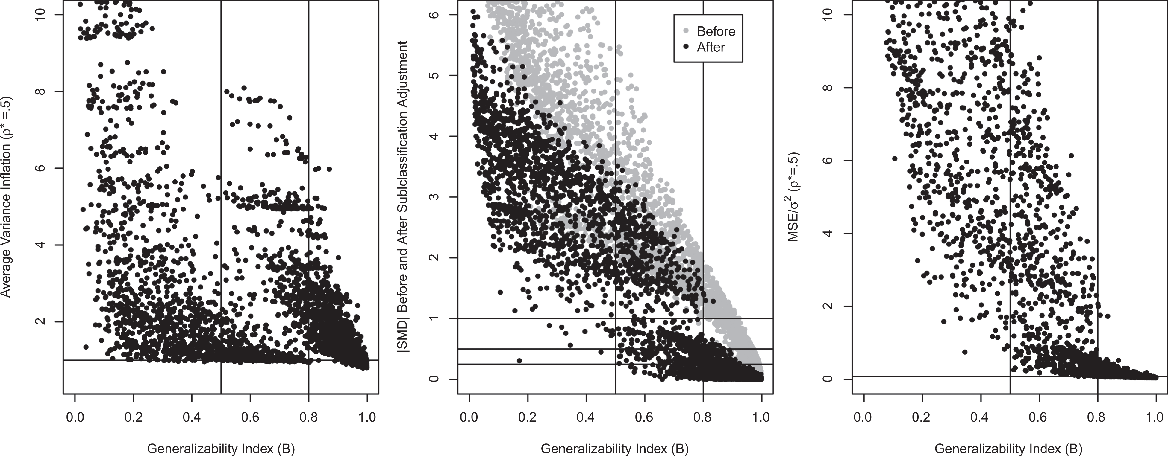

\begin{matrix} A = \sum_{j = 1}^{k} \frac{w_{p_{j}}^{2}}{w_{s_{j}}} & C = \sum_{j = 1}^{k} \frac{w_{p_{j}}^{2}}{w_{s_{j}}} \frac{s_{s_{j}}^{2}}{s_{s}} \\ D = \frac{{\overset{ˉ}{X}}_{s} - {\overset{ˉ}{X}}_{p}}{s_{p}} & E = \frac{\sum_{j = 1}^{k} w_{p_{j}}^{} {\overset{ˉ}{X}}_{s_{j}} - {\overset{ˉ}{X}}_{p}}{s_{p}} \end{matrix}

\begin{aligned} E V I F = A (1 - ρ^{* 2} (1 - C / A)) \\ M S E / γ^{2} = D^{2} + (4 / n) E V I F . \end{aligned}

Here the quantity A is the maximum average variance inflation (max EVIF) due to reweighting, while C is the minimum EVIF (min EVIF), and the EVIF is a weighted combination of the two (based here on an assumed value of ρ* = ½). Additionally, here D is the SMD estimated before reweighting and E is the SMD based on a subclassification estimator with k equal population strata. Finally, MSE/γ² is the value of the scaled MSE (i.e., bias² + variance). Derivations of these formulas can be found in the Online Appendix and involve the same simplifying assumptions found in Tipton (2013).

Figure 2 illustrates the relationship between B and each of these quantities using three plots; in each plot, vertical lines are included for B = (.50, .80). The leftmost plot relates B to the average variance inflation when ρ* = ½ (i.e., EVIF), which indicates a moderate relationship between the propensity score and outcomes. As this plot indicates, when B ≥ .80, the expected variance inflation is not large and ranges from smaller than 1 (indicating that variance is reduced, as occurs often in poststratification estimators with small adjustments) to just around 6, with most values less than 2. When B is between .50 and .80, these values range much more, from around 1 to closer to 10, with an average closer to 3. For values of B < .50, however, the degree of inflation can be quite large. Although not indicated on this graph, the maximum inflation is actually upward of 30. In many cases, this inflation is so large because the two distributions do not overlap well (both φ < 1 and θ < 1) and the reweighting estimator dramatically reduces the available sample size in the experiment, that is, (1 − ϕ)n cases receive zero weight (w _pj = 0).

The second plot in Figure 2 relates B to the SMD before and after subclassification (with k strata). Two trends are immediately obvious here. First, as B increases, the SMD decreases. This relationship is not perfect, however, and as the plot indicates, the same value of the initial SMD can be related to a wide range of B values; for example, when the initial SMD is 2, values of B can range from as low as .40 to as high as .82. Second, reweighting reduces this bias best when B ≥ .80. Here the final bias is most often less than 1 and very often less than .50 or .25. Third, when B < .80, while bias reduction is possible for all values of B, the amount of remaining bias can be high. When .50 < B ≤ .80, this bias can often, but not always, be reduced to a SMD less than 1 (or smaller); but in some cases, the resulting bias is still large. Clearly, when B < .50, however, the resulting bias is always greater than 1 SD.

Finally, the third plot combines the relationship between variance inflation and bias reduction into a combined measure of “usefulness”—the MSE. In this plot, B is related to the MSE/γ² when the value of ρ*² (relating the propensity scores and outcomes) is a moderate ρ*² = ½. Here a horizontal line indicates the associated value if the sample was a random sample from the population (i.e., if MSE/γ² = 4/n). In this plot, it is clear that when B ≥ .80, the MSE/γ² value is smallest and is most affected by the degree of variance inflation (since bias reduction is large); while for values of B < .80, the MSE/γ² value is much larger, since the degree of bias dominates. These values are particularly large when B < .50, indicating estimates that are not particularly useful in terms of indicating PATE.

Although developing rules of thumb is always difficult, the results of these simulation studies suggest that four possible categories may be helpful in generalization:

very high: 1.00 ≥ B ≥ .90;

high: .90 > B ≥ .80;

medium: .80 > B ≥ .50; and

low: B < .50.

Here “very high” generalizability means that the experimental sample is “like” a random sample from the population of interest. When the sample is not like the population, however, reweighting can be used to estimate a useful result when the sample has “high” generalizability. This means that the reweighted estimate of PATE is likely to be close to conditionally unbiased (assuming that the ignorability condition has been met) and that the sample is sufficiently similar to the population that this reweighting will result in only a small increase in standard errors. In contrast, when a sample is considered to have “medium” generalizability, while reweighting is possible, as a result of coverage errors or overlap problems, the reweighted estimator will contain bias and/or the inflation to the standard errors could be large. This means that results may not be quite as useful. Finally, for those with “low” generalizability, the sample and population are considered sufficiently different that no amount of reweighting will produce a useful estimate of the average treatment effect for the population. In some cases, this is because the amount of bias that can be removed is very small, and/or (though typically both) the resulting standard errors will be so large as to deem the reweighted estimate “useless.” In the next section, we illustrate these rules of thumb and further investigate properties of B through an example.

Example

The most common way we envision the B index being used is to indicate how similar an experimental sample is to multiple populations; this is what is often referred to as narrow to broad generalizations (Shadish, Cook, & Campbell, 2002). As an example, we turn to the Success for All (SFA) reading program evaluation that started in 2001–2003. In their evaluation, Borman et al. (2005) included a list of the 41 schools included in the experiment. This included elementary schools in 12 states located throughout all four regions of the United States (Southeast, Northeast, Midwest, and West), and the stated goal of the sample recruitment was to generalize to the population of schools implementing SFA at that time.

In this example, we define 51 separate inference populations—one for each state and the District of Columbia—using the 2002–2003 Common Core of Data (National Center for Education Statistics). Further information on the example is found in the Online Appendix (see Supplement Example Note 1). For each of the 51 inference populations, we compare the 41 schools in the experiment to the population by estimating the sampling propensity score. To do so, we use a logistic regression model including a set of eight covariates (see Supplement Example Note 2). For each of the populations, the B index is calculated based on the propensity score logits. The results are depicted visually in Figure 3, which also includes points locating the 41 schools that took part in the experiment (see Supplement Example Note 3). Importantly, this map illustrates that the degree of generalizability does not necessarily correspond to the locations of the schools in the experiment. For example, the degree of similarity is high for Michigan, despite the fact that there were no experimental schools in the state; this is in contrast to Arizona, where the degree of generalizability is low, despite its representation in the experiment.

Figure 3.

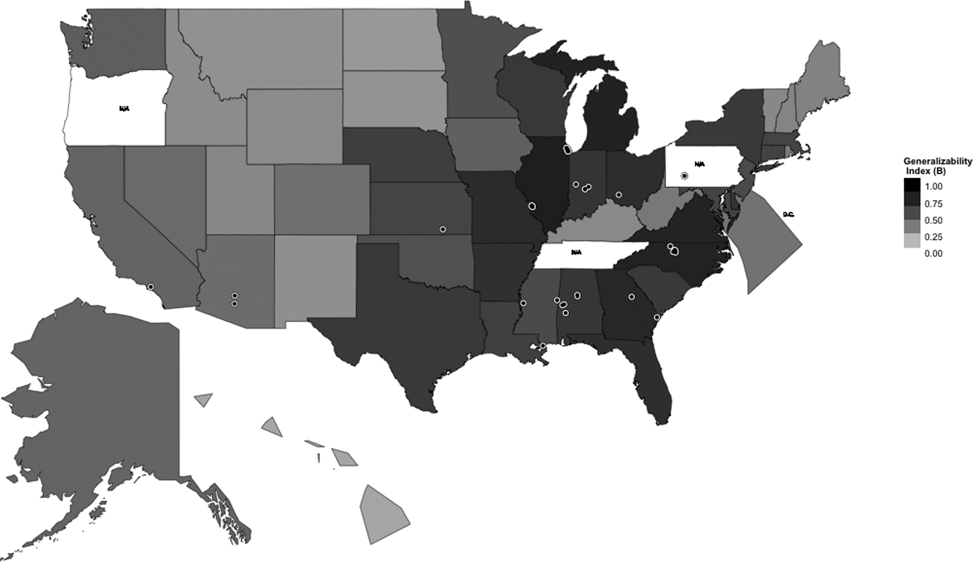
Where do the results of the Success for All (SFA) experiment generalize?

Table 1 provides further information on this example. Note that while the SFA study does not generalize well to all states, it does have a high degree of generalizability to the population of Title I eligible schools in the United States overall (B = .80). Importantly, the study sample is not similar enough to any of the states or the combined United States to be considered “like” a random sample. However, in addition to the United States, in three states the degree of generalizability is high, indicating that reweighting could be implemented with little cost in terms of residual bias and variance inflation, namely, Illinois, Michigan, and North Carolina.

Table 1 also reports measures in addition to B. In practice, these would not be required but are useful here as a way to further explore the properties of B. The middle third of the table includes the four alternative measures of generalizability provided by Stuart et al. (2011)—the SMD (in propensity scores and in logits), the average propensity difference, and the variance ratio. The furthest columns to the right also include calculations regarding how successful a reweighting strategy might be in terms of bias reduction and variance inflation.

In Table 1, there are several interesting trends. First, the SMD values found here are much larger than the rules of thumb indicating similarity (“balance”) in the quasi-experimental literature (e.g., Rubin, 2001). Although they are typically lowest for states with high generalizability index values, the SMD alone does not indicate how “good” of a final estimator may be possible for the average treatment effect. For example, while the SMD for Texas is 1.85 (the eighth smallest value), poststratification here is particularly effective in removing bias (i.e., k = 4 equal population strata are possible), reducing the final SMD to .41. However, this bias reduction comes at a large cost in terms of variance inflation—the estimator produced by this reweighting would have a variance of over 2.65 times as large as the naive estimator. This bias–variance combination is captured by the B index value of .67, indicating “medium” generalizability. In contrast, in North Carolina, the SMD is only slightly smaller (1.53), and the reweighting is only slightly more effective (k = 4 strata), reducing the SMD to .36. Here, however, the cost in terms of variance inflation is dramatically smaller: an expected inflation of 59% versus 165%. Again, this bias–variance combination is captured by the B index value of .80, indicating “high” generalizability. Further discussion of these results can be found in the Online Appendix (see Supplement Example Note 4).

Conclusion

In this article, we propose an index that can be used to assess how similar an experimental sample is to an inference population. The index that we propose, β (and its estimator B), is a natural extension to the visual comparison of histograms common in propensity score analyses. As such, the relationship between β and generalizability is dependent on the covariates included in the propensity score model. For this reason, it is important that these covariates are clearly defined and discussed in relation to β.

As the example illustrates, one important feature of this β index is that it can be used to quickly and easily compare how generalizable a sample is to a variety of different inference populations. Importantly, the index is easy to interpret and explain to a lay audience. This is largely because it corresponds easily to the visual comparison of histograms but also because it addresses three important issues, namely, sampling and coverage (θ), relevant sample size (φ), and compositional similarity (β₀). Although each of these three components is interesting in itself, for lay audiences it is their combination that matters, since together they provide information on the usefulness of experimental results for a population of policy interest.

Furthermore, the fact that this index can be calculated independent of information on the outcomes means that the issue of generalizability can be separated from issues of study design or analysis. This means that the index can be useful in other situations as well, including the assessment of similarity during the sample selection process outlined by Tipton (2014). As Tipton et al. (2014) highlight, in many experiments there are eligibility criteria. For example, researchers often limit their site selection efforts to a few states or one state, yet wish to make generalizations to a broader audience (e.g., the United States). The generalizability index could be used to determine which states or regions were most compositionally similar to this larger population, thus increasing generalizability.

Finally, we have focused throughout on the use of β as an index of similarity between a sample and a population. However, the definitions of β (or the Hellinger distance, η = $\sqrt{1 - β}$ ; Hellinger, 1909; see Online Appendix) could just as easily be used as measures of similarity or distance in propensity score analyses in quasi-experiments. Doing so would allow the differences detected in histograms to be reduced to a single number, providing more information than the SMD commonly used.

Footnotes

Declaration of Conflicting Interests

The author(s) declared no potential conflicts of interest with respect to the research, authorship, and/or publication of this article.

Funding

The author(s) disclosed receipt of the following financial support for the research, authorship, and/or publication of this article: NSF grant#1118978.

Note

Supplemental Material

The online Appendix is available at

References

Aherne

F. J.

Thacker

N. A.

Rockett

P. I.

(1998). The Bhattacharyya metric as an absolute similarity measure for frequency coded data. Kybernetika, 34, 363–368.

Bareinboim

Pearl

(2013). A general algorithm for deciding transportability of experimental results. Journal of Causal Inference, 1, 107–134.

Bhattacharyya

(1943). On a measure of divergence between two statistical populations defined by their probability distributions. Bulletin of the Calcutta Mathematical Society, 35, 99–109.

Bhattacharyya

(1946). On a measure of divergence between two multinomial populations. Sankhya: The Indian Journal of Statistics, 7, 401–406.

Belitser

S. V.

Martens

E. P.

Pestman

W. R.

Groenwold

R. H. H.

de Boer

Klungel

O. H.

(2011). Measuring balance and model selection in propensity score methods. Pharmacoepidemiology and Drug Safety, 20, 1115–1129.

Borman

G. D.

Slavin

R. E.

Cheung

Chamberlain

A. M.

Madden

N. A.

Chambers

(2005). Success for all: First-year results from the national randomized field trial. Educational Evaluation and Policy Analysis, 27, 1–22.

Chattopadhyay

A. K.

Rao

C. B.

(2009). Bhattacharyya’s distance measure as a precursor of genetic distance measures. Journal of Biosciences, 29, 135–138.

Chernoff

(1952) A measure of asymptotic efficiency of tests for hypothesis based on a sum of observations. Mathematical Statistics, 23, 493–507.

Comaniciu

Ramesh

Meer

(2000). Real-time tracking of non-rigid objects using mean shift. Proceedings of the IEEE Conference on Computer Vision and Pattern Recognition, 2, 142–149.

10.

Cornfield

Tukey

J. W.

(1956). Average values of mean squares in factorials. The Annals of Mathematical Statistics, 27, 907–949.

11.

Franklin

J. M.

Rassen

J. A.

Ackermann

Bartels

D. B.

Schneeweiss

(2014). Metrics for covariate balance in cohort studies of causal effects. Statistics in Medicine, 33, 1685–1699.

12.

Greenburg

Schroder

(2004). The digest of social experiments (3rd ed.). Washington, DC: The Urban Institute Press.

13.

Groves

R. M.

Fowler

F. J.

Couper

M. P.

Lepkowski

J. M.

Singer

(2009). Survey methodology. New York, NY: John Wiley.

14.

Hedges

L. V.

O’Muircheartaigh

C. A.

(2011). Improving generalizations from designed experiments (Working Paper). Evanston, IL: Northwestern University.

15.

Hellinger

(1909). Neue Begrundung der Theorie quadratischer Formen von unendlichvielen Veranderlichen. J Reine Angew Math, 36, 210–271.

16.

D. E.

Imai

King

Stuart

E. A.

(2007). Matching as nonparametric preprocessing for reducing model dependence in parametric causal inference. Political Analysis, 15, 199–236.

17.

Jensen

J. L. W. V.

(1906). Sur les fonctions convexes et les inegalites entre les valeurs moyennes. Acta Mathematica, 30, 175–193.

18.

Khalid

M. S.

Ilyas

M. U.

Sarfaraz

M. S.

Ajaz

M. A.

(2006). Bhattacharyya coefficient in correlation of gray-scale objects. Journal of Multimedia, 1, 56–61.

19.

Kitagawa

E. M.

(1964). Standardized comparisons in population research. Demography, 1, 296–315.

20.

Matusita

(1967). On the notion of affinity of several distributions and some of its applications. Annals of the Institute of Statistical Mathematics, 19, 181–192.

21.

Nummiaro

Koller-Meier

Van Gool

(2003). An adaptive color-based particle filter. Image and Vision Computing, 21, 99–110.

22.

Olsen

R. B.

Orr

L. L.

Bell

S. H.

Stuart

E. A.

(2013). External validity in policy evaluations that choose sites purposively. Journal of Policy Analysis and Management, 32, 107–121.

23.

O’Muircheartaigh

Hedges

L. V.

(2014). Generalizing from unrepresentative experiments: A stratified propensity score approach. Journal of the Royal Statistical Society: Series C (Applied Statistics), 63, 195–2010.

24.

R Development Core Team. (2014). R: A language and environment for statistical computing. R Foundation for Statistical Computing, Vienna, Austria. ISBN 3-900051-07-0. Retrieved from http://www.R-project.org/

25.

Rao

C. R.

(1949). On the distance between two populations. Sankhyā: The Indian Journal of Statistics, 9, 246–248.

26.

Rao

C. R.

(1982). Diversity and dissimilarity coefficient: A unified approach. Theoretical Population Biology, 21, 24–43.

27.

Raudenbush

S. W.

Bryk

A. S.

(2002). Hierarchical linear models: Applications and data analysis methods (2nd ed.). Volume 1 of Advanced Quantitative Techniques in the Social Sciences. Newbury Park, CA: Sage.

28.

Rosenbaum

P. R.

Rubin

D. B.

(1983). The central role of the propensity score in observational studies for causal effects. Biometrika, 70, 41–55.

29.

Rubin

D. B.

(1974). Estimating causal effects of treatments in randomized and nonrandomized studies. Journal of Educational Psychology, 66, 688–701.

30.

Rubin

D. B.

(2001). Using propensity scores to help design observational studies: Application to the tobacco litigation. Health Services & Outcomes Research Methodology, 2, 169–188.

31.

Rubin

D. B.

Thomas

(1996). Matching using estimated propensity scores: Relating theory to practice. Biometrics, 52, 249–264.

32.

Shadish

W. R.

Cook

T. D.

Campbell

D. T.

(2002). Experimental and quasi-experimental designs for generalized causal inference. Boston, MA: Houghton-Mifflin.

33.

Shen

Nelson

D. E.

Kennedy

Spiller

D. G.

Griffiths

… Kell

D. B.

(2006). Automated tracking of gene expression in individual cells and cell compartments. Journal of The Royal Society Interface, 3, 787–794.

34.

Silverman

B. W.

(1986). Density estimation for statistics and data analysis (Vol. 26). Boca Raton, FL: CRC Press.

35.

Stuart

(2010) Matching methods for causal inference: A review and a look forward. Statistical Science, 25, 1–21.

36.

Stuart

E. A.

Cole

S. R.

Bradshaw

C. P.

Leaf

P. J.

(2011). The use of propensity scores to assess the generalizability of results from randomized trials. Journal of the Royal Statistical Society, Series A, 174, 369–386.

37.

Stuart

E. A.

Olsen

R. B.

Bell

S. H.

Orr

L. L.

(2012). Estimates of external validity bias when impact evaluations select sites purposively. Proceedings from the Society for Research on Annual Effectiveness Spring Meeting, Washington, DC .

38.

Tipton

(2013). Improving generalizations from experiments using propensity score subclassification: Assumptions, properties, and contexts. Journal of Educational and Behavioral Statistics, 38, 239–266.

39.

Tipton

(2014). Stratified sampling using cluster analysis: A balanced-sampling strategy for improved generalizations from experiments. Evaluation Review, 37, 109–139.

40.

Tipton

Hedges

L. V.

Vaden-Kiernan

Borman

Sullivan

Caverly

(2014). Designing a sample selection plan to improve generalizations from two scale-up experiments. Journal of Research on Educational Effectiveness, 7, 114–135.

41.

Zhang

Wang

(2009). A new distance-based approach for phylogenetic analysis of protein sequences. International Journal of Biology and Biomedical Engineering, 3, 35–42.

Supplementary Material

Please find the following supplemental material available below.

For Open Access articles published under a Creative Commons License, all supplemental material carries the same license as the article it is associated with.

For non-Open Access articles published, all supplemental material carries a non-exclusive license, and permission requests for re-use of supplemental material or any part of supplemental material shall be sent directly to the copyright owner as specified in the copyright notice associated with the article.

0.00 MB

0.13 MB