A Survey of Popular R Packages for Cluster Analysis

Abstract

Cluster analysis is a set of statistical methods for discovering new group/class structure when exploring data sets. This article reviews the following popular libraries/commands in the R software language for applying different types of cluster analysis: from the stats library, the kmeans, and hclust functions; the mclust library; the poLCA library; and the clustMD library. The packages/functions cover a variety of cluster analysis methods for continuous data, categorical data, or a collection of the two. The contrasting methods in the different packages are briefly introduced, and basic usage of the functions is discussed. The use of the different methods is compared and contrasted and then illustrated on example data. In the discussion, links to information on other available libraries for different clustering methods and extensions beyond basic clustering methods are given. The code for the worked examples in Section 2 is available at http://www.stats.gla.ac.uk/∼nd29c/Software/ClusterReviewCode.R

Keywords

cluster analysis k-means hierarchical clustering model-based clustering

1. Introduction

Cluster analysis is an area of statistics involved with finding groups in data by aggregating items that are similar in some sense into separate classes (Everitt, Landau, Leese, & Stahl, 2011). Any field that has interest in finding meaningful groups within data could benefit from statistical clustering. Some recent applications have included using clustering to group student skill set profiles (Dean & Nugent, 2013), to group rates of obesity and diabetes in U.S. counties (Flynt & Daepp, 2015), and to estimate the spatial patterns in disease risk (Anderson, Lee, & Dean, 2014).

This article discusses a selection of libraries and commands in the R software language (R Core Team, 2015) for implementing some of the most popular methods for algorithmic and parametric clustering. The structure of the remainder of this article is as follows: In Section 2, we briefly review the models/algorithms for k-means and hierarchical clustering (subsection 2.2), model-based clustering (MBC), and latent class analysis (LCA; subsection 2.3) and introduce the package/commands for implementing these methods. We apply the different packages to example data and review the relevant output before concluding with a discussion in Section 3 and pointers toward other packages for further cluster analysis extensions. Note that R commands and libraries will be indicated with this font, while the command arguments will be indicated with an alternative font.

2. Common Cluster Analysis Methods and Their Implementation

Given that data are clustered such that the objects within groups found are similar in some way(s), there are obviously different methods for defining similarity. For example, one of the most popular methods for defining dissimilarity is using Euclidean distance from the cluster center which leads to the k-means method, or using the density of points in the surrounding area that leads to MBC. The many different definitions of (dis)similarity have led to a wide variety of clustering methodologies. These can be roughly divided into three main categories: algorithmic, parametric, and nonparametric. Some of the oldest cluster analysis methods such as k-means (MacQueen, 1967) and hierarchical clustering (Ward, 1963) are examples of the algorithmic class of methods. Methods such as MBC (Wolfe, 1963; Fraley & Raftery, 2002) and LCA (Lazarsfeld, 1950a, 1950b; Lazarsfeld & Henry, 1968), based on finite mixture models (McLachlan & Peel, 2000), are examples of parametric clustering. Nonparametric clustering (mentioned again in Section 3) looks to identify modes in the estimated density surface for the data with clusters.

We now introduce the simulated data set used to illustrate the cluster analysis methods described and implemented in the remaining subsections. Code and selected output will be presented that can be adapted for the reader’s own data analysis.

2.1. Data

To illustrate the discussed R packages, we will present results from a simulated data set of 600 observations with two continuous variables and four discrete (three binary and one ternary) variables. The continuous variables, named vars, create three underlying groups, two of which are spherical and one elliptical. These simulated groups can be seen in Figure 1a (177 observations in black, 237 in red, and 186 in green). The binary variables, named c1, c2, c3, were simulated in such a way that one variable had uniform probability of success across the groups, another had higher success probability for the black group, and the final had higher success probability for the red group. In the ternary variable, c4 there was a higher probability of being assigned a 1 in the black group, a 2 in the red group, and a 3 in the green group. The exact distribution of these variables within each underlying group can be seen in Figure 1b. Throughout the remainder of this section, the estimated clustering from each method will be compared to the true simulated groups, named by their color in Figure 1a.

Figure 1.

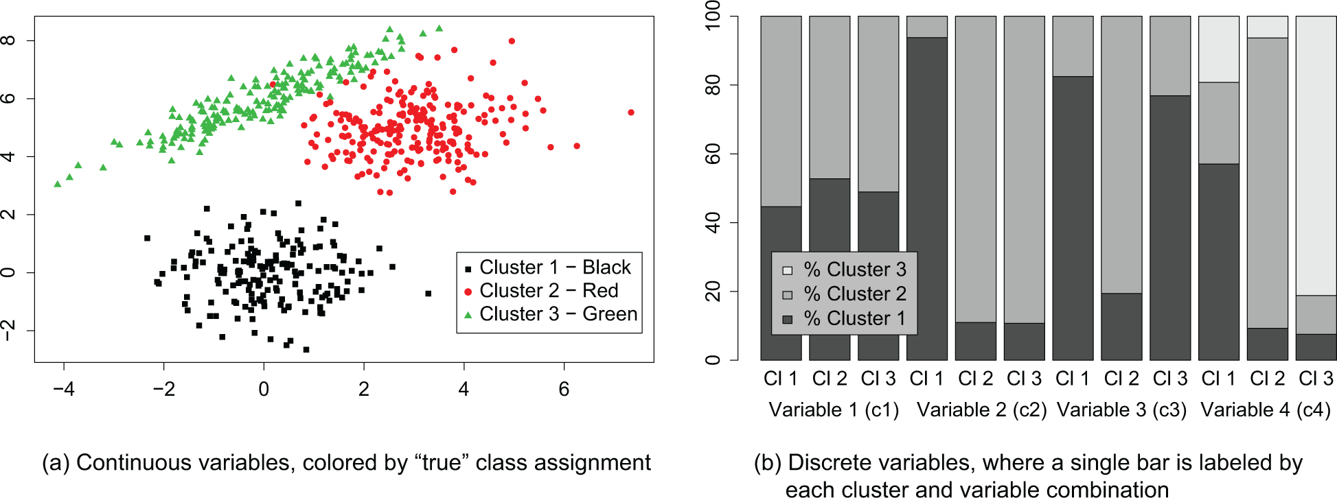
Simulated data set.

In the following sections, R code to be implemented is prefaced by the prompt symbol > (which would be omitted if copying this into an R console), comments and output not meant to be implemented are prefaced by #.

2.2. Algorithmic Clustering Methods

2.2.1. k-Means

k-Means is based on the idea that points should be assigned to the clusters that minimize the overall distance between points and the cluster means/centroids to which they have been assigned. The typical distance measure used is Euclidean (although other distances can theoretically be used), so the method is usually only applied to continuous data. k-Means assumes the variability in all clusters in all variables is the same, resulting in the discovery of spherical clusters which each take up an equal volume in variable space. If variables are measured on vastly different scales, it is a good idea to scale them prior to applying k-means; the R command scale can be used to automatically center and/or scale vectors. The most common command for implementing k-means in R is the kmeans command located in the stats library.

One of the issues in any clustering method is the decision as to how many clusters are present in the data being examined. The most common way to choose the number of clusters for k-means is by fitting k-means models for a range of consecutive numbers, usually 1 up to some maximum number, and plotting an elbow plot of the total within sum of squares value for each number of clusters versus that cluster number. An example is given in Figure 2 in subsection 2.2.2. The number of clusters is taken to be the “elbow” or turning point in the line plot where the reduction in sum of squares seems to drop off. 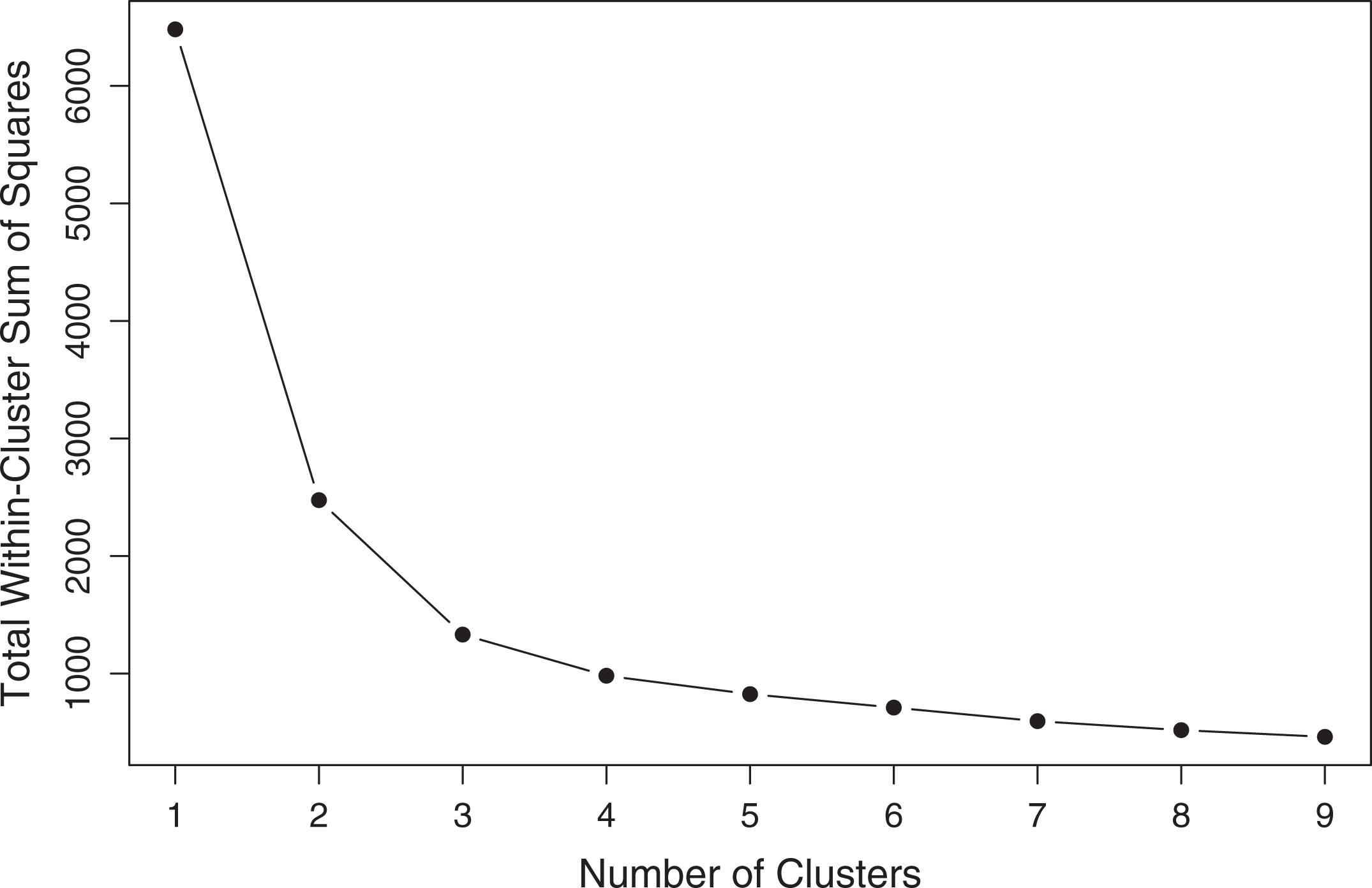The assignment of points into clusters for a particular model is obtained by extracting the cluster assignment, cluster, in the resulting fitted object list.

Figure 2.

Elbow plot for the total within-cluster sum of squares from k-means models.

Other nonvisual methods for choosing the number of clusters (for any clustering method, not just k-means) are performed by calculating some metric that measures goodness of aspects of the clustering. Examples of these measures found in the fpc library (Hennig, 2015) are average silhouette width, the Calinski and Harabasz index, and a Pearson version of Hubert’s gamma coefficient.

2.2.2. Simulated data results and code for k-means

The first argument in the kmeans command is the data matrix (rows = observations, columns = variables), then the second argument, centers, can either be set to the number of clusters required or a matrix of data points representing the initial cluster centers. The default value for the argument nstart, which specifies how many times the algorithm is run with random starts before choosing the best result, is 1, which is not to be advised. A larger value, at least 10 or more if time allows, particularly as the dimensionality/number of variables rises, is to be recommended.

Here we run k-means for different values of k, from 1 to 9, with 50 random starts on the first two columns/continuous variables in our simulated data set vars.

# Running kmeans on the two continuous variables for various k

> km1 = kmeans(vars[,1:2], 1, nstart = 50)

> km2 = kmeans(vars[,1:2], 2, nstart = 50)

> km3 = kmeans(vars[,1:2], 3, nstart = 50)

> km4 = kmeans(vars[,1:2], 4, nstart = 50)

> km5 = kmeans(vars[,1:2], 5, nstart = 50)

> km6 = kmeans(vars[,1:2], 6, nstart = 50)

> km7 = kmeans(vars[,1:2], 7, nstart = 50)

> km8 = kmeans(vars[,1:2], 8, nstart = 50)

> km9 = kmeans(vars[,1:2], 9, nstart = 50)

# Create the elbow plot of the within sum of squares for each k versus the value k

> plot(1:9, c(km1$tot.withinss, km2$tot.withinss, km3$tot.withinss, km4$tot.withinss,

+ km5$tot.withinss, km6$tot.withinss, km7$tot.withinss, km8$tot.withinss,

+ km9$tot.withinss), type = 'b', pch = 19, xlab = 'Number of Clusters',

+ ylab = 'Total Within-Cluster Sum of Squares', main = '', xaxt = 'n',

+ cex.axis = .75)

> axis(1, 1:9, 1:9, cex.axis = .75)

# Look at the output for the fitted k-means object for k = 3 clusters

> km3

# k-means clustering with 3 clusters of sizes 177, 163, 260

# Cluster means:

# 1 0.1140557 -0.04430671

# 2 -0.4616140 5.59210875

# 3 2.9434956 5.27018783

# Clustering vector:

### Not shown for reasons of space, prints the cluster assignment of each of the points

# Within cluster sum of squares by cluster:

# [1] 342.7049 340.3659 648.1870

# (between_SS / total_SS = 79.5 %)

# Available components:

# [1] 'cluster' 'centers' 'totss' 'withinss' 'tot.withinss' 'betweenss'

# [7] 'size' 'iter' 'ifault'

# Cross-classification table where cl is the simulated class assignment and km$cluster

# is the vector of cluster assignments; here the rows are the true classes, the columns

# the k-means clusters, entries in the table indicate how many observations fall in each

# combination of class and cluster number

> table(cl, km3$cluster)

# cl 1 2 3

# 1 177 0 0

# 2 0 10 227

# 3 0 153 33

The elbow plot from the resulting k-means models can be seen in Figure 2. This plot suggests the choice of the three-cluster model. It is common to create a cross-classification table (see table in output) comparing the true simulated groups and the estimated clusters. Note that the estimated clusters may have labels switched from the true groups (as seen above) but can be reordered appropriately. The misclassification rate is calculated as the number of misclassified observations out of the total number of observations. We see that for the three-cluster solution produced by k-means, the black group was perfectly recovered, but 43 observations were misclassified in the overlapping red and green groups, resulting in a misclassication rate of $43 / 600 = 0.071 \bar{6}$ .

2.2.3. Hierarchical agglomerative clustering

Hierarchical agglomerative clustering is based on the idea of successively merging the pair of closest/most similar clusters together to form a new larger cluster until all points are merged into one cluster. Usually, the order and height of merges are visualized in a tree-like diagram called a dendrogram (sometimes dendogram; see, e.g., Figure 3). The advantage of this method is the ability to easily visualize the structure of the data regardless of how high dimensional it may be. This method of clustering also allows for hierarchy in the clusters found.

Figure 3.

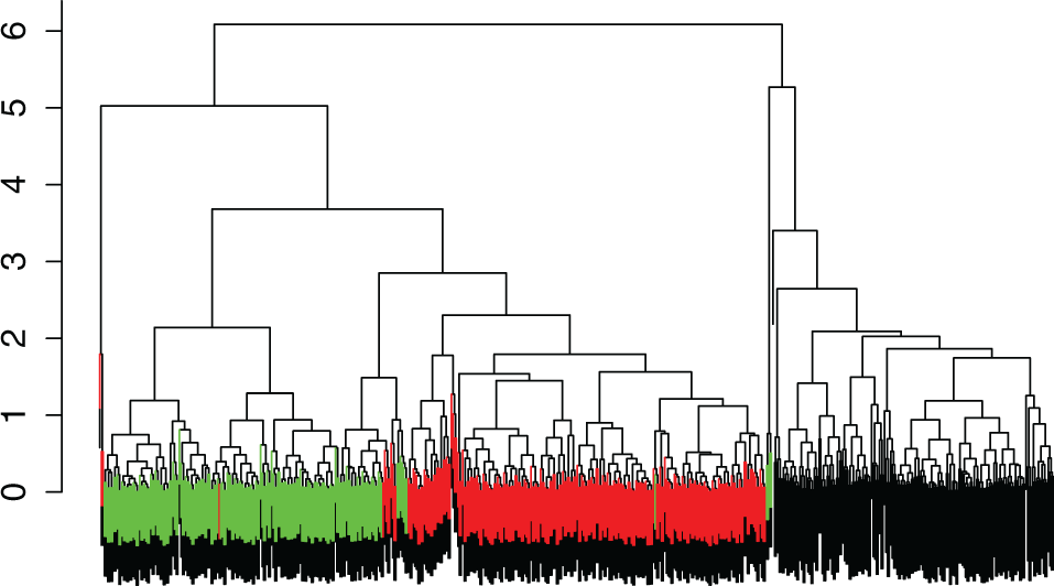
Colored dendrogram resulting from hierarchical clustering using average linkage.

There are several ways to calculate linkages: the distance between pairs of nonsingelton clusters. Each definition of linkage gives rise to a different type of clustering solution on the same data. Single linkage defines the distance between two clusters as the minimum of all the pairwise distances between pairs of points in the different clusters. This type of linkage gives rise to “chaining,” where the merges are more likely to have points or small clusters joining with a large cluster rather than forming new large clusters. This effect can lead to groups that are of unusual shape (e.g., nonspherical and nonelliptical) but can also lead to close groups being incorrectly merged if there is any degree of overlap. Single linkage is usually very useful in identifying outliers. This linkage is also related to the minimal spanning tree (see Gower & Ross, 1969, for details). Complete linkage is the maximum of the pairwise distances between all pairs of points in the different clusters. It tends to separate out overlapping groups well but will do poorly recovering nonstandard shapes of groups. Average linkage uses the average pairwise distance between all pairs of points in the different clusters as the measure of distance. The clustering for average linkage usually lies somewhere between the solutions given by single and complete linkage. Centroid linkage defines distance between clusters as the distance between the cluster centroids. Ward’s linkage looks at the increase in sum of squared deviations from cluster means before and after a merge, as the measure of similarity. This linkage tends to find compact spherical clusters similar to k-means clustering.

2.2.4. Simulated data results and code for hierarchical clustering

Hierarchical agglomerative clustering in R is generally carried out using the hclust command in the stats library.

The first argument is a distance object, containing all the pairwise distances between points in the data set. This can be created using the dist function. If the dist function is not used, then the as.dist function may be needed to force the object into the correct format. The next argument is the linkage method (e.g., method = “complete”). The plot command plots a dendrogram, and a colored dendrogram can be produced using the ColorDendrogram function in the sparcl library (Figure 3). The command cutree is used to classify the data points into the clusters where the fitted dendrogram is cut with either the number of clusters or the height at which the tree should be cut.

Figure 3 shows a colored dendrogram of the results from hierarchical clustering with average linkage. If we choose to cut the tree at three clusters, the black group is completely recovered, but the green group is almost entirely merged into the red group, resulting in a misclassification rate of 0.30. The code for implementing this is given below.

# Note the first argument must be a distance matrix

> h2 = hclust(dist(vars[,1:2]), method = 'average')

# To see the result

> h2

# Call:

# hclust(d = dist(vars[, 1:2]), method = 'average')

# Cluster method : average

# Distance : euclidean

# Number of objects: 600

# To produce a dendrogram

> plot(h2)

# To produce a colored dendrogram

> ColorDendrogram(h2, y = cl, main = '', xlab = '', sub = '')

# cutree will classify the data points into the clusters where the fitted dendrogram

# is cut. Can specify the number of clusters like below, or the height at which to

# cut the tree with h =

# Cut the dendrogram here to give k = 3 clusters

> h2cut = cutree(h2, k = 3)

# Produce a cross-classification table comparing true classes, cl, to the cluster

# assignments in h2cut

> table(cl, h2cut)

# cl 1 2 3

# 1 0 177 0

# 2 237 0 0

# 3 182 0 4

2.3. Clustering Methods Based on Finite Mixture Models

MBC, a parametric method, is based on estimating a statistical model rather than optimizing a function. The model on which MBC and LCA is based is the finite mixture model (McLachlan & Peel, 2000). Instead of modeling the data as a single population with a single distribution, the finite mixture model assumes that the population is made up of multiple subpopulations. Each of the subpopulations has an associated weight equal to its associated proportion in the whole population as well as a component-specific distribution that models the data in the subpopulation. The density for the data is then given by the following equation:

f (x) = \sum_{k = 1}^{K} τ_{k} f_{k} (x), 0 \leq τ_{k} \leq 1, \sum_{k = 1}^{K} τ_{k} = 1.

Here τ _k is the kth mixing proportion equal to the proportion this component subpopulation makes up of the whole population and f_k () is the kth component density. Usually, the component densities all come from the same parametric family. The expectation-maximization (EM) algorithm (Dempster, Laird, & Rubin, 1977) is used to estimate the model parameters. It is common for each component to be associated with a cluster. The probability of belonging to each component is calculated for each observation, and the observation can be assigned to the component/cluster for which it has largest probability of membership.

Often, the number of components that best fits the data is equivalent to the number of clusters present in the data, so that choosing the number of clusters becomes a model-choice problem, with different numbers of clusters/components defining a different model. The most common way to identify the best fitting number of components is to fit different models for a range of numbers of clusters, score each model, and select the model with the best score. The most common scoring measure used is the Bayesian Information Criterion (BIC; Schwarz, 1978), which can be calculated in a number of different ways. If calculated for model M as

BIC (M) = 2 \log (maximized likelihood of model M) - v \log (n),

(where v is the number of independent parameters in model M and n is the number of observations), then the number of components that maximizes the BIC score is considered the best fit. If the BIC definition is −1× the definition given above, then the minimum is considered best.

2.3.1. MBC

MBC is the common name for finite mixture model clustering for continuous data. In MBC, the component density f_k is Gaussian with corresponding mean and variance estimates. That is, each component can be summarized by a mean, variance, and a mixing proportion.

2.3.2. Simulated data results and code for MBC

In MBC, the unrestricted variance matrix for component k is high dimensional and difficult to estimate, so the mclust package fits different variance matrix parameterizations. For univariate data, the options are “E” or “V” (equal or variable across components), and a variety of different options exist for multivariate data indexed by three letters “XXX,” the first letter indicating the volume of the components, either E or V; the second letter indicating the shape of the components, E or V or “I” (for the identity matrix); and the third letter indicating the orientation of the components, E, V, or I. k-Means is similar to the model with either E for univariate or “EII” for multivariate data. In the mclust library (Fraley, Raftery, Murphy, & Scrucca, 2012), the function Mclust is used to fit the finite mixture model.

The first argument for the Mclust command is the data matrix, the second is the range of number of components to be fit (default is 1 to 9), and the best model chosen is the one with the highest BIC value. The identified best model (in terms of variance parameterization and number of components, see Figure 4a) can be found by using the summary command on the fitted Mclust object. The classification element of the fitted mclust object gives the assignment of data points to clusters (e.g., fit$classification).

# Fit the mbc model for a range of number of components, default 1 to 9 and all

# variance parameterizations on the continuous variables

> m1 = Mclust(vars[,1:2])

# Look at which model is selected by BIC

> m1

# 'Mclust’ model object:

# best model: ellipsoidal, equal orientation (VVE) with 3 components

# Look at the summary of the model

> summary(m1)

# ----------------------------------------------------

# Gaussian finite mixture model fitted by EM algorithm

# ----------------------------------------------------

# Mclust VVE (ellipsoidal, equal orientation) model with 3 components:

# log.likelihood n df BIC ICL

# -2230.702 600 15 -4557.359 -4572.325

# Clustering table:

# 1 2 3

# 229 177 194

# Look at the BIC, classification and other plots for this model (type ‘0’ to exit plotting)

> plot(m1)

# Look at the cross-classification table for the cluster assignments, given by m1$class

# and the true labels, cl.

> table(cl, m1$class)

# cl 1 2 3

# 1 0 177 0

# 2 229 0 8

# 3 0 0 186

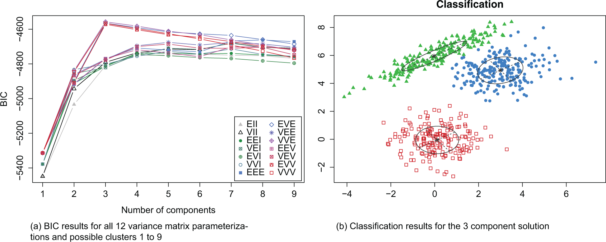
The three-component model with variance matrix parameterization “VVE” had the highest BIC. The plot function can be used on an Mclust object to view four different plots: BIC (Figure 4a), classification (Figure 4b), uncertainty, and density. This method correctly clusters all but eight of the observations from the red group by assigning them to the green group (misclassification rate = $0.01 \bar{3}$ ), as seen in the cross-classification table above.

Figure 4.

Two example plots produced by Mclust.

2.3.3. LCA

LCA is the common name for finite mixture model clustering for categorical data. LCA assumes conditional independence for the variables given component membership, that is, all the variables are independent within the clusters (but not marginally independent) similar to the “XXI” models in the continuous case for MBC. Each variable within each component is modeled by a multinomial variable. Each component can be summarized using the proportions for each category in each variable (as well as the mixing proportion).

On a technical note, a necessary (but not sufficient) condition for identifiability of a G component/class/cluster LCA model to be fit to data with k variables, each having levels d_i , i = 1,…, k is:

d_{1} \times d_{2} \times \dots \times d_{k} > (d_{1} + d_{2} + ⋯ + d_{k} - k + 1) \times G .

2.3.4. Simulated data results and code for LCA

In the poLCA library (Linzer & Lewis, 2011), the poLCA command is used to fit the LCA model. Similar to kmeans, one should fit a range of consecutive numbers for nclass and choose the model with the lowest values of reported Akaike information criterion (AIC) or BIC scores.

The first argument in the poLCA command is a formula with the data to be clustered (variables in columns) on the left separated by a tilde from a 1 on the right, for example, data∼1. The assignment of points to their estimated class can be found in the predclass element of the fitted poLCA object (e.g., fit$predclass).

# Must specify a formula with the data to be clustered (variables in columns)

# on the left separated by a tilde from a 1 on the right

> f = cbind(c1, c2, c3, c4)∼1

> lca1 = poLCA(f, data.frame(vars), nclass = 1)

> lca2 = poLCA(f, data.frame(vars), nclass = 2)

> lca3 = poLCA(f, data.frame(vars), nclass = 3, maxiter = 3500)

> lca4 = poLCA(f, data.frame(vars), nclass = 4, maxiter = 21000)

# maxiter for the 3 and 4 class models needed to be increased for convergence

# Create an elbow plot for the number of classes and the BIC values

> plot(1:4, c(lca1$bic, lca2$bic, lca3$bic, lca4$bic), type = 'b',

+ pch = 19, xlab = 'Number of Clusters', ylab = 'BIC', main = '', xaxt = 'n')

> axis(1, 1:4, 1:4)

# To look at the outcome for the 3-class fit

> lca3

# Conditional item response (column) probabilities, by outcome variable,

# for each class (row)

# $c1

# Pr(1) Pr(2)

# class 1: 0.5149 0.4851

# class 2: 0.4152 0.5848

# class 3: 0.5208 0.4792

# $c2

# Pr(1) Pr(2)

# class 1: 0.2617 0.7383

# class 2: 0.8206 0.1794

# class 3: 0.1384 0.8616

# $c3

# Pr(1) Pr(2) Pr(3)

# class 1: 0.0000 0.0000 1.0000

# class 2: 0.7507 0.2493 0.0000

# class 3: 0.0810 0.8763 0.0427

# $c4

# Pr(1) Pr(2)

# class 1: 0.7818 0.2182

# class 2: 0.8756 0.1244

# class 3: 0.2015 0.7985

# Estimated class population shares

# 0.3151 0.2581 0.4268

# Predicted class memberships (by modal posterior prob.)

# 0.3333 0.2567 0.41

# =======================================================================

# Fit for 3 latent classes:

# =======================================================================

# number of observations: 600

# number of estimated parameters: 17

# residual degrees of freedom: 6

# maximum log-likelihood: -1722.435

# AIC(3): 3478.87

# BIC(3): 3553.618

# G⁁2(3): 4.992174 (Likelihood ratio/deviance statistic)

# X⁁2(3): 4.944048 (Chi-square goodness of fit)

# To obtain the assignment of points to their estimated class

> lca3$predclass

# Cross-classification table for the predicted classes versus the true labels

> table(cl, lca3$predclass)

# cl 1 2 3

# 1 34 129 14

# 2 15 12 210

# 3 151 13 22

The elbow plot illustrating the BIC results for fitting an LCA model to the discrete variables for one to four clusters is given in Figure 5. Note that lower BIC is better here. This plot suggests the use of three clusters. Because the underlying simulated groups were less defined by the discrete variables (see subsection 2.1), this model has a higher misclassification rate of $0.18 \bar{3}$ .

Figure 5.

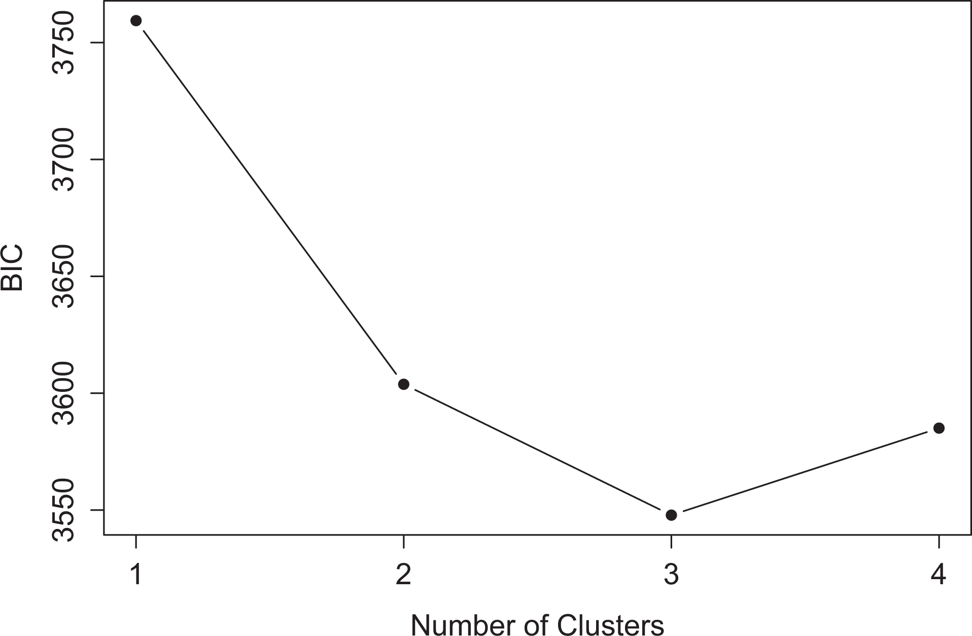
Elbow plot for poLCA models fit on one to four clusters.

2.3.5. MBC for mixed data

The clustMD library (McParland, 2015) presents an elegant MBC approach to grouping sets of data with all types of variables: continuous, binary, ordinal, and nominal. Coding of categorical variables must start at 1 and increase by unit increments. The noncontinuous variables are modeled as categorizations of unseen latent Gaussian variables in the item response theory vein. However, the MBC approach means that within each cluster, latent variables are modeled by their own Gaussians, different to that in other clusters. This results in a finite mixture model of both observed continuous variables and unobserved/latent Gaussian variables. As with the mclust approach, parsimony is achieved by restricting elements of the variance matrices across the clusters. (The models available are “EII,” “VII,” “EEI,” “VEI,” “EVI,” or “VVI” in the same fashion as mclust.)

2.3.6. Simulated data results and code for MBC for mixed data

The first argument of clustMD is the data matrix, which must order the columns with first, the continuous variables, followed by the binary, ordinal, and then nominal variables (except in cases where there are nonesuch). The second argument identifies the number of components to fit, the third says how many continuous variables are in the data set, and the fourth says how many total variables there are in the data. The argument model is a string entry indicating which of the parsimonious models are to be used.

The function clustMD is used on the full set of six variables, which are continuous and discrete. This mixed model is fit for a range of one to four groups and all combinations of the six available variance matrix parameterizations.

# Specify variance matrix parameterizations to be used - here all

> methods = c('EII', 'VII', 'EEI', 'VEI', 'EVI', 'VVI')

# Set the range of the number of clusters

>clust.range = c(1:4)

# Initializing storage of the BIC

> mds.bic = matrix(NA, nrow = length(clust.range), ncol = length(methods))

# In clustMD, the columns of the data matrix must be ordered: continuous, binary,

# ordinal and then nominal variables (except in cases where there are nonesuch)

# CnsIndx is the number of continuous variables

# OrdIndx is the total number of variables

# Looping through the 6 variance parameterizations for 1:4 classes (saving BIC)

> for(m in methods){

+ for(g in clust.range){

+ mds.bic[g, which(methods==m)] = clustMD(X = vars, G = g, CnsIndx = 2, OrdIndx = 6,

+ Nnorms = 100, MaxIter = 500, model = m, scale = FALSE)$BIChat

+ }

# Fitting the model with the highest BIC

> md.min = clustMD(vars, G = 4, CnsIndx = 2, OrdIndx = 6, Nnorms = 100, MaxIter = 500,

+ model = 'EEI', scale = FALSE)

# Assignment of points to their estimated classes is given in md.min$cl

# Produce cross-classification table between true classes and assigned clusters

> table(cl, md.min$cl)

# cl 1 2 3 4

# 1 0 177 0 0

# 2 231 0 4 2

# 3 1 0 79 106

The model with the highest BIC (see Figure 6a) was the four-cluster solution with parameterization EEI. As seen in Figure 6b where observations are colored by their estimated cluster, this model has essentially split the original green group into two clusters and resulted in a misclassification rate of $0.14 \bar{3}$ .

Figure 6.

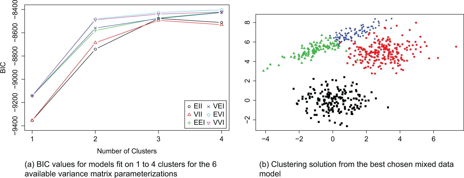
Results for clustMD models.

3. Discussion

As illustrated in Section 2, different clustering methods applied to the same data can produce vastly different results. It is difficult to recommend which method will work in practice since different group/data types will require different methods and it is seldom obvious a priori which is optimal. There is no one cluster method that is best in every situation, unfortunately. Cluster analysis as discussed in this article should be considered an exploratory analysis, and we recommend replicating/validating cluster results on one data set with a later data set of the same type before making any definitive statements.

In general, single linkage hierarchical clustering should really only be used for the identification of outliers because it is rarely useful otherwise. Sometimes the type of cluster solution you want should be driven by substantive reasons, rather than by the data. If one believes a genuine hierarchy of clustering solutions for the data, hierarchical clustering is then preferred. If long, elongated clusters do not make substantive sense (do you want a cluster with wide variability in one variable and not others?), then general MBC models might be avoided in favor of spherical models (like EII and VII or k-means or Ward’s linkage hierarchical clustering).

Although a full survey of the available extensions outside of the basic models/algorithms already introduced is beyond the scope of this article, we offer references to a few popular alternatives and extensions.

3.1. Alternative Methods

An alternative to k-means that does not use the centroid as a measure of the center of the cluster but instead uses an actual central data point is called k-medoids. This is useful when you want real data points as the prototypes for the clusters found. The command for implementing this in the cluster library (Maechler, Rousseeuw, Struyf, Hubert, & Hornik, 2015) is pam (short for partitioning around medoids).

Instead of agglomerative merging, it is also possible to have a divisive version of hierarchical clustering which starts with all observations in one cluster and successively splits clusters in two. This is not generally as popular as the agglomerative version, but the command diana in the cluster package executes this algorithm.

As an alternative to MBC of mixed data, one can define a distance measure on the continuous and categorical variables and apply distance methods such as hierarchical clustering (as discussed previously) if preferred. Hennig and Liao (2013) gives a good example of how to construct such a measure in a principled fashion.

3.2. Extensions

Due to space limitations, this article does not discuss extensions on clustering methodology like clusterwise regression (see the package flexmix, Gruen & Leisch, 2008, for fitting such models as finite mixtures of regression models or some commands in the poLCA library for the same idea for categorical data), or variable selection (see clustvarsel, an add-on package to mclust or Rmixmod, Auder, Lebret, Iovleff, & Langrognet, 2014, for implementation of wrapper methods for variable selection for cluster methods), or combining mixture components to create multicomponent clusters (see the clustCombi command in mclust for an example of this implementation). Also, an example of a package implementing nonparametric clustering, that we mentioned in the introduction but do not review, is pdfCluster (Azzalini & Menardi, 2014).

One of the most up-to-date resources for finding cluster analysis packages on R is the CRAN Task View page on Cluster Analysis and Finite Mixture Models found at http://finzi.psych.upenn.edu/views/Cluster.html. It provides short summaries of the functionalities of all the packages currently known to be available for clustering in R and is updated on a regular basis. Many of the packages mentioned also provide in-depth vignettes that give more detail on their usage. Finally, the R command example is useful for automatically running the example code in help files for package commands to give an idea of how the command is to be used (e.g., example(kmeans)).

Footnotes

Declaration of Conflicting Interests

The author(s) declared no potential conflicts of interest with respect to the research, authorship, and/or publication of this article.

Funding

The author(s) received no financial support for the research, authorship, and/or publication of this article.

References

Anderson

Lee

Dean

(2014). Identifying clusters in Bayesian disease mapping. Biostatistics, 3, 457–469.

Auder

Lebret

Iovleff

Langrognet

(2014). Rmixmod: An interface for MIXMOD (R package Version 2.0.2).

Azzalini

Menardi

(2014). Clustering via nonparametric density estimation: The R package pdfCluster. Journal of Statistical Software, 57, 1–26.

Dean

Nugent

(2013). Clustering student skill set profiles in a unit hypercube using mixtures of multivariate betas. Advances in Data Analysis and Classification, 3, 339–357.

Dempster

A. P.

Laird

N. M.

Rubin

D. B.

(1977). Maximum likelihood from incomplete data via the EM algorithm. Journal of the Royal Statistical Society. Series B (Methodological), 39, 1–38.

Everitt

Landau

Leese

Stahl

(2011). Cluster analysis. Wiley Series in Probability and Statistics. Chichester, England: Wiley.

Flynt

Daepp

M. I.

(2015). Diet-related chronic disease in the northeastern United States: A model-based clustering approach. International Journal of Health Geographics, 14, 25.

Fraley

Raftery

A. E.

(2002). Model-based clustering, discriminant analysis, and density estimation. Journal of the American Statistical Association, 97, 611–631.

Fraley

Raftery

A. E.

Murphy

T. B.

Scrucca

(2012). Mclust version 4 for r: Normal mixture modeling for model-based clustering, classification, and density estimation. Technical Report 597, Department of Statistics, University of Washington.

10.

Gower

J. C.

Ross

G. J. S.

(1969). Minimal spanning tree and single linkage cluster analysis. Journal of the Royal Statistical Society, Series C (Applied Statistics), 18, 54–65.

11.

Gruen

Leisch

(2008). Flexmix version 2: Finite mixtures with concomitant variables and varying and constant parameters. Journal of Statistical Software, 28, 1–35.

12.

Hennig

(2015). fpc: Flexible procedures for clustering (R package Version 2.1-10).

13.

Hennig

Liao

T. F.

(2013). How to find an appropriate clustering for mixed type variables with application to socioeconomic stratification. Journal of the Royal Statistical Society, Series C (Applied Statistics), 62, 309–369.

14.

Lazarsfeld

P. F.

(1950a). Measurement and prediction, volume IV of the American soldier: Studies in social psychology in World War II, chapter the logical and mathematical foundations of latent structure analysis (pp. 362–412). Princeton, NJ: Princeton University Press.

15.

Lazarsfeld

P. F.

(1950b). Measurement and prediction, volume IV of the American soldier: Studies in social psychology in World War II, chapter some latent structures. Princeton, NJ: Princeton University Press.

16.

Lazarsfeld

P. F.

Henry

N. W.

(1968). Latent structure analysis. Boston, MA: Houghton Mifflin.

17.

Linzer

D. A.

Lewis

J. B.

(2011). poLCA: An R package for polytomous variable latent class analysis. Journal of Statistical Software, 42, 1–29.

18.

MacQueen

(1967). Some methods for classification and analysis of multivariate observations. In Le Cam

L. M.

Neyman

(Eds.), Proceedings of the fifth Berkeley symposium on mathematical statistics and probability, volume 1: Statistics (pp. 281–297). Berkeley: University of California Press.

19.

Maechler

Rousseeuw

Struyf

Hubert

Hornik

(2015). Cluster: Cluster analysis basics and extensions (R package Version 2.0.3).

20.

McLachlan

G. J.

Peel

(2000). Finite mixture models. New York, NY: Wiley.

21.

McParland

(2015). clustMD: Model based clustering for mixed data (R package Version 1.1).

22.

R Core Team. (2015). R: A language and environment for statistical computing. Vienna, Austria: R Foundation for Statistical Computing.

23.

Schwarz

G. E.

(1978). Estimating the dimension of a model. Annals of Statistics, 6, 461–464.

24.

Ward

J. H.

(1963). Hierarchical grouping to optimize an objective function. Journal of the American Statistical Association, 58, 236–244.

25.

Wolfe

J. H.

(1963). Object cluster analysis of social areas. Master’s thesis, University of California, Berkeley.