
Abstract
This article describes the analysis of regression-discontinuity designs (RDDs) using the
Keywords
The regression-discontinuity design (RDD) was first considered by Thistlethwaite and Campbell (1960). Despite some initial interest in the method, it never became a very popular design choice (Cook, 2008). There is, however, a current renaissance of the RDD, fueled in part by important theoretical contributions from economics (Angrist & Pischke, 2009; Imbens & Kalyanaraman, 2012). In this literature, the RDD is often considered to be one of the strongest nonrandomized designs with regard to drawing causal conclusions from data. As a result of these advances, there is now also an increased interest in performing RDDs among applied researchers, especially in economics and education (Louie, Rhoads, & Mark, 2016; Melguizo, Bos, Ngo, Mills, & Prather, 2016; Porter, Reardon, Unlu, Bloom, & Cimpian, 2016; Zhang, Hu, Sun, & Pu, 2016).
Introductions to the underlying logic and analysis of the RDD are numerous (Imbens & Lemieux, 2008; Lee & Lemieux, 2010; Schochet et al., 2010; Trochim, 1984); therefore, we will keep our theoretical presentation very short. The RDD is a design that facilitates causal identification of an effect T, on an outcome Y, in the presence of confounding due to unobserved variables. The key feature of RDDs is an assignment variable, X, that (often uniquely) defines treatment assignment T. For example, the treatment could be enrollment in a remedial math class, and the assignment variable is a score on a standardized math test. Here, school administrators assign students to the math class, if and only if, the math score of a particular student is below a certain threshold.
If the assignment variable X deterministically causes the treatment, we refer to this as a sharp RDD. If the relationship between X and T is only probabilistic (meaning that the probability of receiving the treatment does not switch from 0 to 1 at the cutoff of X but to some other values ranging between 0 and 1, e.g., .1 or .9), we refer to this as a fuzzy RDD. The relationship between X and Y is allowed (and expected) to be confounded by unobserved variables. However, even in the presence of unobserved confounding, it is possible to estimate an unbiased causal effect, if the data are analyzed properly using RDD methods. The exact reasons why the RDD can yield unbiased effects have been spelled out by Shadish, Cook, and Campbell (2002) using the language of the generalized causal inference framework by Campbell, or by Imbens and Lemieux (2008) using the language of potential outcomes. We provide here a simple explanation using graphical causal models (Pearl, 2009).
Consider the graphical model in Figure 1, which consists of variables (nodes in the graph) and paths (arrows in the graph). Directed paths indicate causal relationships, and bidirected paths indicate confounding relationships due to unobserved variables. Consider now that we are interested in the causal effect of T on Y. In the graph in Figure 1, the relationship between T and Y is confounded, due to the presence of X and the (countless) unobserved variables that induce an association between X and Y (the bidirected path). However, the graph also informs us that every unobserved variable influences T only through X and that X alone determines T. In some sense, X is a “bottleneck” for all potentially confounding influences between T and Y. As such, conditioning on X is sufficient to deconfound the relationship between T and Y and thus obtain an unbiased causal effect.

Graphical causal model of a regression-discontinuity design.
Another way to understand why the RDD yields results similar to those of a randomized experiment is to consider the fact that individuals who are right below the cutoff of the assignment variable and right above the cutoff of the assignment variable are expected to be very similar to each other (we may also say that they are exchangeable). They only differ on treatment assignment. Consider the hypothetical data shown in Figure 2, in which every individual who scored lower than 0 on the assignment variable X is assigned to the treatment condition, whereas everyone who scored equal or higher than 0 is assigned to the control condition. The individuals who are closely around this cutoff are indeed comparable with respect to X and presumably other variables as well. They only differ with respect to the treatment assignment. As a result, the data in this area that is close to the cutoff resemble a randomized experiment, which allows the identification of a causal treatment effect.
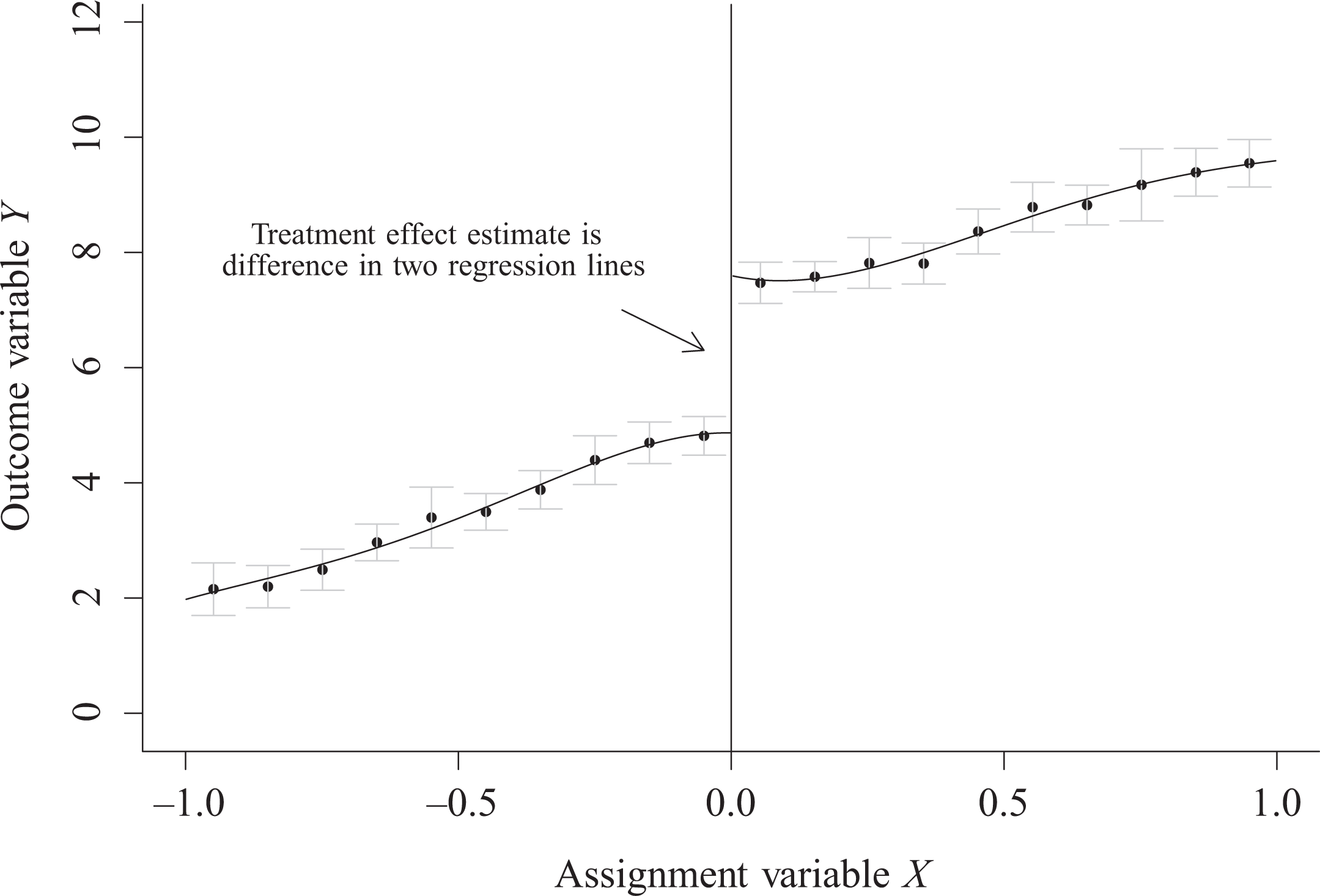
Example plot of data in a regression-discontinuity design, created using the
Conceptual Overview of an RDD Analysis
The statistical analysis of RDDs is described in much detail elsewhere (Imbens & Lemieux, 2008; Lee & Lemieux, 2010; Schochet et al., 2010; Trochim, 1984), and it is not the focus of this article to formally describe these analyses. Nevertheless, it is helpful to at least give a brief overview of the involved analyses, before considering the exact implementation of them in the
We consider a scenario, in which a researcher has identified a variable that acts as an assignment variable in an RDD that allows identification of a causal effect of interest. As a concrete example, a researcher may have identified that a local agency administers an enrichment program at schools, but only to students whose grades are below a certain threshold, for example, a grade point average (GPA) below 2.5. The researcher wants to know whether providing the enrichment has any effect on later learning, and therefore collects data on students’ GPAs, later learning outcomes, and whether they have attended the enrichment program.
Assumption Checks
In a first step, the researcher would have to confirm that the design assumptions of the RDD were not violated. In particular, this means confirming that the treatment assignment mechanism behaved as assumed. For example, there may be concerns that students with slightly higher GPAs were also allowed to participate in the enrichment program, by changing their records slightly. Or maybe parents could petition that their child would be allowed to participate even if the child’s GPA made it ineligible. Those violations could be visible in discontinuities (essentially “bumps”) in the distribution of the assignment variable, here GPA. These discontinuities can be visually inspected or formally tested with a hypothesis test (McCrary, 2008).
Second, one would assume that the treatment effect only occurs at the cutoff of GPA 2.5 and not at other cutoffs. If we would in fact observe treatment effects at other cutoffs, we would feel less confident that the presumed treatment effect is really due to the treatment that was administered differentially at the cutoff. A formal way to explore this is to estimate treatment effects at various other cutoffs and compare them with the effect at the presumed cutoff. This procedure is sometimes referred to as “placebo tests.”
Third, the treatment is believed to have an impact on an outcome variable but not on nonoutcome covariates, especially those collected prior to treatment administration. In fact, if we would observe a treatment effect on a pre-treatment covariate, much doubt would be cast on the validity of the RDD. To formally explore this, researchers are encouraged to replace the actual outcome with each of the covariates and redo the RDD analysis. A desired result would be that no effect at the cutoff is found in any of the pretreatment covariates.
Estimation
Assuming that all assumption checks were successful, a researcher may now estimate the treatment effect. The treatment effect of an RDD is quantified in the difference between regression lines right at the cutoff. In the example at hand, the researcher would have to estimate the jump in the regression line relating GPA to later academic outcomes right at the cutoff of a GPA 2.5, at which the treatment assignment switched. This effect estimation is achieved either through parametric regression models (also known as the global approach) or through semi- or nonparametric methods, which often only consider points close to the cutoff through weighting and employing local linear or local polynomial regression (also known as the local approach). If researchers choose to employ the global, parametric approach, it is often suggested that higher order polynomials should be fitted, although there are opposing viewpoints (Gelman & Imbens, 2014). The parametric models are parameterized in such a fashion that one of the resulting coefficients expresses the discontinuity in the regression line, usually achieved through centering the assignment variable and forming interaction terms. If the local, nonparametric approach is chosen, only data points closely around the cutoff are chosen and a local linear (or local polynomial) regression model is fitted on either side of the cutoff. Usually, these models are fitted using weighted regression, giving higher weights to individuals who are closer to the cutoff. A challenging question is how to choose the bandwidth that determines these weights. The most popular choice is a data-driven bandwidth selection algorithm first suggested by Imbens and Kalyanaraman (2009). In Imbens and Kalyanaraman (2012), this selection algorithm is further modified. More recent developments have added additional choices for the bandwidth selection (Calonico, Cattaneo, & Farrell, 2016; Calonico, Cattaneo, & Titiunik, 2015b). Simulation studies (Calonico, Cattaneo, & Titiunik, 2014) suggest that these novel choices have good frequentist coverage properties. As explained in much detail in Calonico, Cattaneo, and Titiunik (2015b), these new choices for bandwidth selection attempt to correct for bias due to undersmoothing (bias that emerges because the functional form of the regression lines at the cutoff is not well approximated) and correct standard errors due to uncertainty in the bias correction.
In the preceding section, we did not differentiate treatment effect estimation for sharp and fuzzy RDDs. While there are differences in the actual analysis, the general logic of measuring a difference in regression lines at the cutoff applies to both. In the case of a fuzzy RDD, an additional step is performed such that the actual observed treatment assignment is regressed on the assignment variable conditioning on the cutoff. Then, an RDD is performed on the predicted treatment assignment, as opposed to the actual observed treatment assignment. This so-called two-stage least squares procedure is identical to the instrumental variables estimator.
Sensitivity Checks
The choice of the parametric model in the global approach or the choice of bandwidth for the local approach is critical, and different choices will yield different estimates of the treatment effect. Because of this model dependency on these choices, it is often suggested to perform some sensitivity checks and explore other modeling options and in doing so bound the treatment effect. Some packages provide these checks automatically, but in theory, the user could always perform the checks manually by simply changing the particular parametric model, or the specific bandwidth, and then estimate the effect again.
To conclude, these three conceptual steps—assumption checks, estimation, and sensitivity checks—complete the analysis of an RDD. We now turn to the implementation of this analysis in
R Packages
We first provide an overview of all available
rdd
The
Differences Between RDD Packages
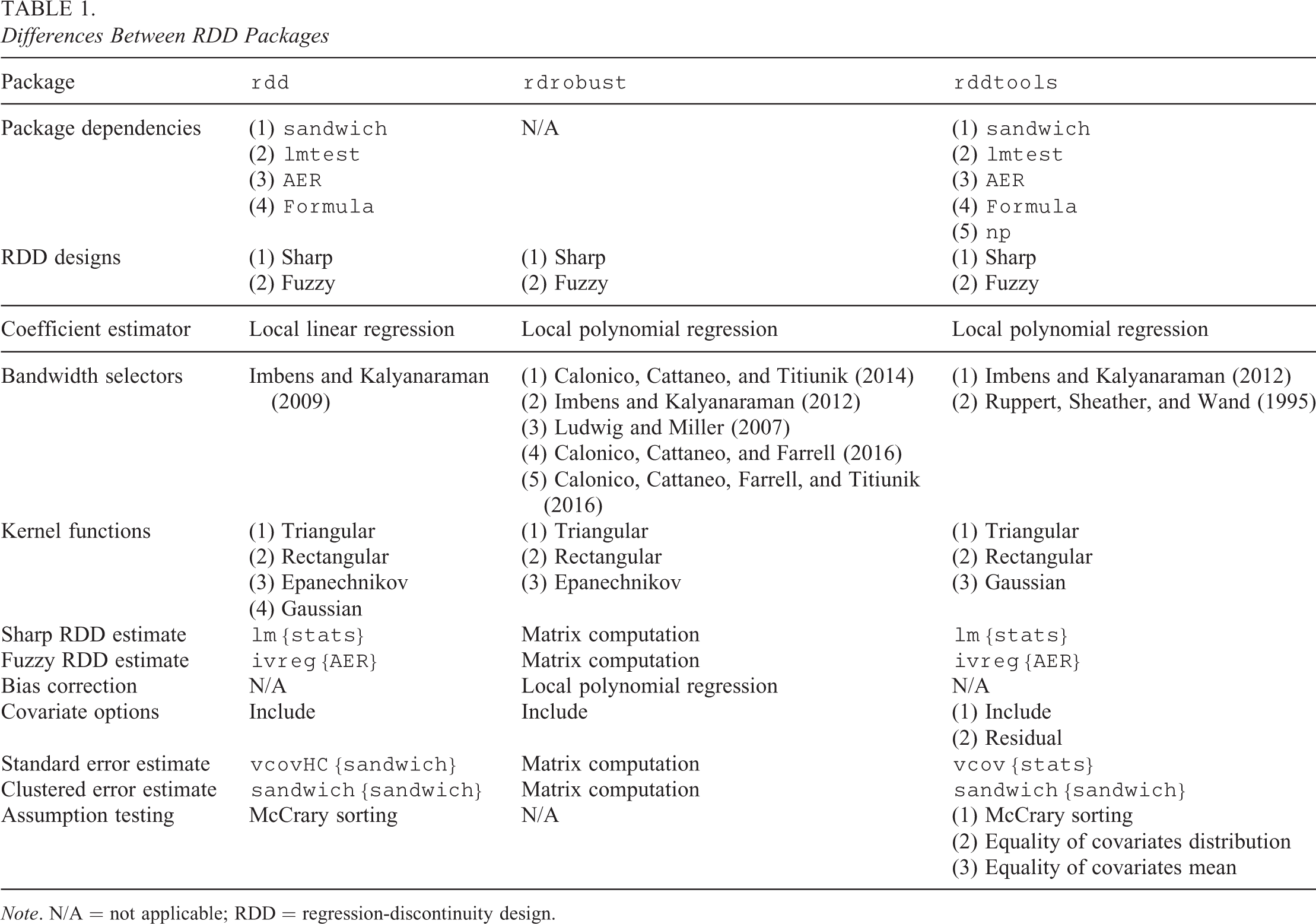
Note. N/A = not applicable; RDD = regression-discontinuity design.
Assumption checks
The
Estimation
The
Sensitivity checks
The
rddtools
The
Assumption checks
The
Estimation
The
Sensitivity checks
The
rdrobust
The
Assumption checks
The
Estimation
Just like all previous packages,
Sensitivity checks
The
Summary of
R
Packages
All three packages are equally easy to use and do not require specialized knowledge of
Finally, for researchers who are less familiar with using packages in
Applied Example
For our applied example, we rely on the published data from the Carolina Abecedarian Project and the Carolina Approach to Responsive Education (Ramey, Gallagher, Campbell, Wasik, & Sparling, 2004), which can be accessed online (http://www.icpsr.umich.edu/icpsrweb/ICPSR/studies/4091). In this randomized controlled trial, young children were assigned to either a control group or to some early childhood intervention, which started at 6 weeks of age and lasted until the third year of elementary school. Children were followed longitudinally for multiple years and were measured on a variety of cognitive measures and academic achievements. The outcome measure that we chose was the Stanford–Binet IQ score at age 2 that was assessed after almost 2 years of treatment. The data set contained 103 children in the control condition and 73 children in the treatment condition. Due to 18 children with missing data on the outcome, only 158 children in total remained. To form a baseline of comparison, we first estimated a treatment effect based on the randomized controlled trial. The mean difference between the two groups was 9.88 IQ points, a highly significant difference, t(156) = 5.46, p = 1.64 × 10⁻⁷, and presumably a very important practical impact.
We then engaged in the following thought experiment: What if the authors of the original study would not have randomly assigned children to conditions, but based on a cutoff on a pretreatment variable? We pretended that treatment was assigned based on such a cutoff. We assumed that treatment would only be administered to mothers whose IQ was below the median of the sample (which in this data set happened to be 85). We took a subset of the data and only retained the treated children whose mothers had an IQ below 85 and the untreated children whose mothers had an IQ of 85 or more. In doing so, we created an RDD out of the randomized controlled trial. This procedure allows us to benchmark our results against the results of the randomized controlled trial. Figure 3a shows a scatterplot of the relationship between mother’s IQ and child’s IQ at 2 years with overlaid locally weighted scatterplot smoothing (LOWESS) smoothers for both treated and untreated children in the original data set. Figure 3b shows the same relationship for the reduced data that mimic an RDD.

Plot of the relationship between assignment variable (mother’s IQ) and outcome (child’s IQ) for (a) the full data and (b) the reduced data. Treated children are shown as black triangles, untreated children as gray dots. Two overlaid smoothers with 95% confidence interval and corresponding colors are shown.
A naive (and biased) estimate of the treatment effect on this subset would be to simply compute the mean difference. Here this turned out to be 4.53 IQ points, a nonsignificant result, t(79) = 1.82, p = .072. We now conduct the RDD analysis using the
Assumptions
We first used the
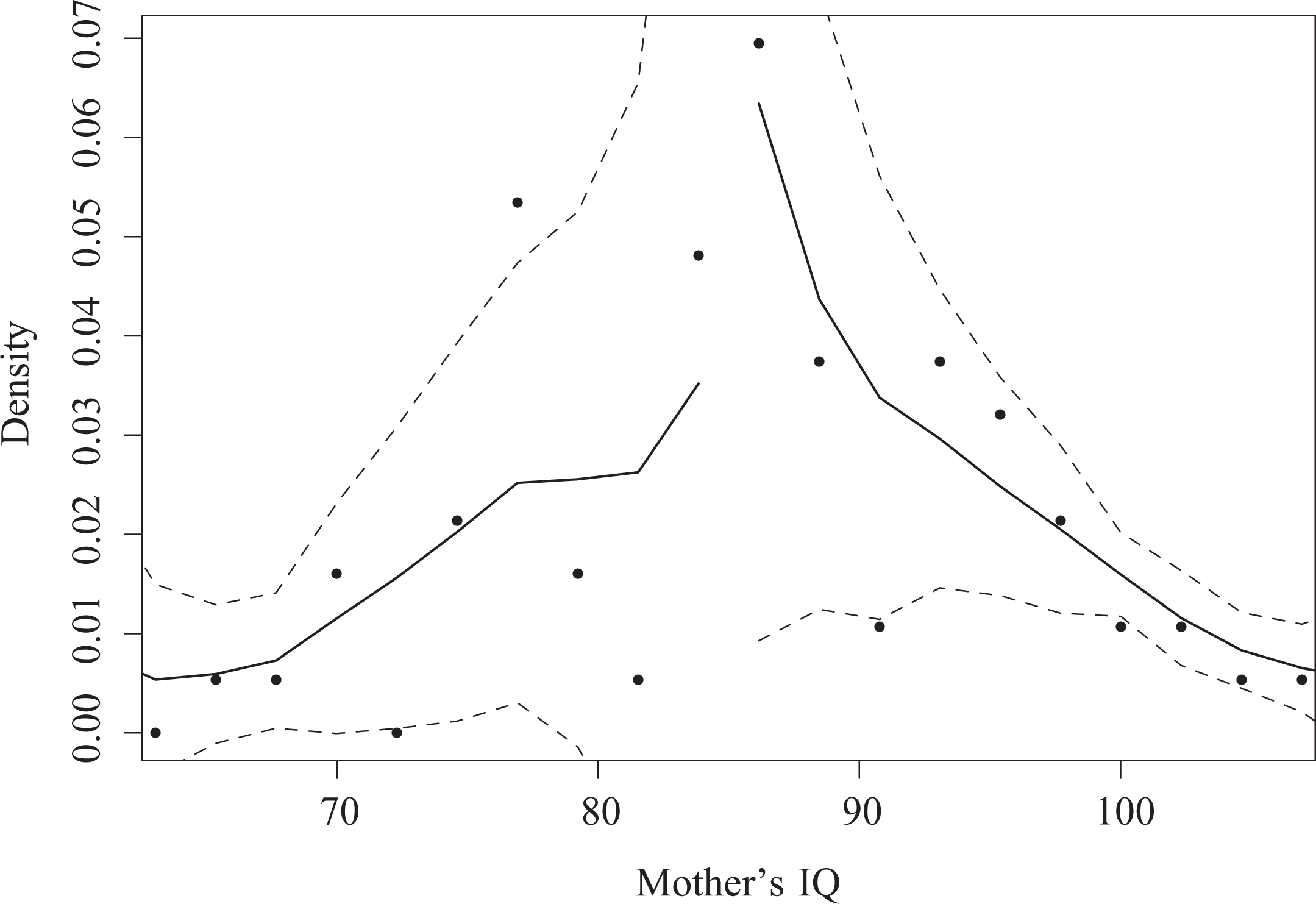
Plot of the density of the assignment variable (mother’s IQ) created using the
A second assumption check is that the treatment effect only occurs at the cutoff. We used the
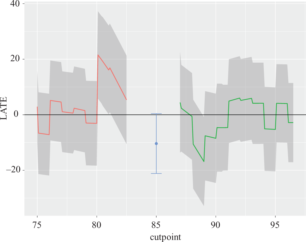
Placebo tests as performed by
In this instance, it appears that some cutoffs also yield similarly sized effects, some even with reversed sign. However, most of the “placebo” cutoffs yield a confidence interval that substantially covers zero, in comparison to the marginal coverage at the actual cutoff. Therefore, the plot suggests some evidence against potential violations in treatment assignment. In real data sets, we might feel inclined to investigate why we might be seeing at least one large effect in the opposite direction at different cutoffs. No other package reports placebo tests.
Finally, we performed a single test of a non-outcome covariate. We chose the Apgar score (a score that identifies how healthy a newborn is). Because it is measured at birth, it is clearly a covariate that was assessed prior to the treatment. An RDD analysis of this non-outcome covariate (using the local approach with default IK bandwidth) found no effect at the cutoff, z(29) = −.08, p = .865. Other non-outcomes could be similarly analyzed to even further increase our confidence in the observed treatment effect.
Estimation
We then proceeded to estimate the treatment effect on IQ at 2 years of age. We first plotted our RDD, using both the

Regression-discontinuity design plot generated in
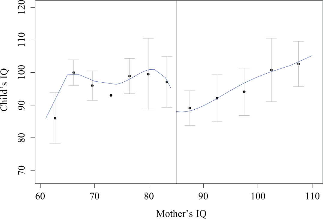
Regression-discontinuity design plot generated in
Both plots show the assignment variable (mother’s IQ) on the horizontal axis and the outcome variable (child’s IQ) on the vertical axis. Both graphs show binned data (bins are formed on the assignment variable, and binned means on the outcome are plotted); however, the binning width is based on different defaults.
2
The plot from the
We then estimated the treatment effect using a wide variety of choices within each of the packages to demonstrate a comprehensive use of them. We have labeled our models M1–M8 and organized our results in Table 2. The table also includes detailed information about bandwidth choices, kernels, types of regression model, sample sizes, and all inferential statistics of the treatment effect. The first model (M1) was estimated using
Estimated Treatment Effects Using Various

Note. RDD assignment is based on mother’s IQ, cut at median (85) with lower scores assigned as treated (i.e., a sharp design). LR = linear regression; IK = Imbens and Kalyanaraman; CCFT = Calonico, Cattaneo, Farrell, and Titiunik; RDD = regression-discontinuity design.
aDefaults to three different estimates. bBias bandwidth and robust p value.
Models M2 through M4 were all estimated using the
Models M5 through M8 were estimated using the
In summary, we can see that treatment effects vary to some extent based on the bandwidth selection. Since different bandwidth selections imply different units that are being considered, it is not surprising that we observed some variability in the estimates. Likewise, we saw that standard errors were generally larger than in the case of the randomized controlled trial (which had a larger sample size). As expected, using narrower bandwidths yielded larger standard errors, and standard errors that were corrected for undersmoothing bias were even larger. At the same time, the general direction and magnitude of the point estimates was consistent with the randomized controlled trial, and generally better than the naive estimate.
Sensitivity checks
Finally, we used the

Sensitivity analysis as performed by
Ideally, we would like to see that the treatment effect remains stable across different choices of bandwidth. As we can see in this plot, the effect remains relatively constant for most choices of bandwidth. With widening bandwidth (toward the right end of the plot), the treatment effect becomes significant (while being of similar magnitude), which is partly due to the increased sample size and the resulting smaller standard error. For very small bandwidths, the estimate becomes highly unstable, which is expected.
Discussion
All packages that we have reported here can be used to analyze an RDD. Many features of the packages are shared and in fact rely on similar underlying dependent
There are, however, features that are currently missing from all of the packages. First, it is impossible to estimate treatment effects from RDDs with multiple assignment variables. Wong, Steiner, and Cook (2013) described situations in which assignment to treatment is not based on a single variable but two (e.g., a remedial classes offered to students who fall below on academic threshold on at least one of the two possible criteria). Wong et al. identify at least four different ways to estimate such effects. Another missing feature is the estimation of statistical power for an RDD. Power considerations are important in RDDs, because statistical power tends to be much lower than in randomized controlled trials (Cappelleri, Darlington, & Trochim, 1994; Goldberger, 1972; Schochet, 2009). Cattaneo, Titiunik, and Vazquez-Bare (2016) have Stata functions and are currently working on putting together an
In summary, there are currently several great packages in
Footnotes
Acknowledgments
The authors would like to thank the editor and reviewers for helpful feedback and the authors of the
Authors’ Note
The opinions expressed are those of the authors and do not represent views of the Institute or the U.S. Department of Education.
Declaration of Conflicting Interests
The author(s) declared no potential conflicts of interest with respect to the research, authorship, and/or publication of this article.
Funding
The author(s) disclosed receipt of the following financial support for the research, authorship, and/or publication of this article: The research reported here was supported by the Institute of Education Sciences, U.S. Department of Education, through Grant R305D150029.
Notes
References
Supplementary Material
Please find the following supplemental material available below.
For Open Access articles published under a Creative Commons License, all supplemental material carries the same license as the article it is associated with.
For non-Open Access articles published, all supplemental material carries a non-exclusive license, and permission requests for re-use of supplemental material or any part of supplemental material shall be sent directly to the copyright owner as specified in the copyright notice associated with the article.