
Abstract
The social relations model (SRM) is a mathematical model that can be used to analyze interpersonal judgment and behavior data. Typically, the SRM is applied to one (i.e., univariate SRM) or two variables (i.e., bivariate SRM), and parameter estimates are obtained by employing an analysis of variance method. Here, we present an extension of the SRM to an arbitrary number of variables and show how the parameters of this multivariate model can be estimated using a maximum likelihood or a restricted maximum likelihood approach. Overall, the two likelihood approaches provide consistent and efficient parameter estimates and can be used to investigate a multitude of interesting research questions.
Keywords
The social relations model (SRM) is a model for group data in which every member of a group has judged all other group members and is also judged by every group member. It is employed in a number of different disciplines including, among others, cognitive science (e.g., Bond, Dorsky, & Kenny, 1992), social and personality psychology (e.g., Kenny, 1994; Küfner, Nestler, & Back, 2012), educational psychology, and developmental psychology. In educational psychology, for example, the SRM was used to examine the performance of pupils in cooperative learning groups (e.g., Horn, Collier, Oxford, Bond, & Dansereau, 1998), whereas developmental psychologists used the SRM to study interdependencies in families (e.g., Ackerman, Kashy, Donellan, & Conger, 2011).
Typically, the SRM is applied to just one variable. For example, groups of individuals judge each other in terms of competence. However, there are a number of research questions, where researchers are interested not only in the analysis of one variable but also in analyzing and relating two or more variables. For example, educational psychologists may be interested not only in analyzing competence judgments but also in the simultaneous analysis of competence judgments, liking judgments, and participating behaviors of pupils. In these cases, an extension of the SRM to multivariate data has to be used. Here, we extend prior research on the estimation of the SRM with likelihood methods (Li, 2006; Li & Loken, 2002; Nestler, 2016; Snijders & Kenny, 1999) and show how the parameters of this multivariate model can be estimated using a maximum likelihood (ML) or a restricted maximum likelihood (REML) approach. Furthermore, we provide an illustrative example and examine the performance of the two likelihood methods in a simulation study.
In the following, we first describe the univariate SRM. We then proceed with a description of the multivariate SRM and the currently used estimation approaches. Thereafter, we explain how the parameters of the model can be estimated using the two likelihood approaches by employing a Fisher scoring algorithm. This is followed by the description of an illustrative empirical example and a simulation study.
The Univariate SRM
Imagine that you are interested in how pupils judge the competence of other pupils. Furthermore, imagine that you have asked different groups of pupils to judge each other in terms of competence (see Table 1 for an excerpt of the resulting data). Such a design, in which every individual of a group judges all other group members in terms of a single variable, is called a univariate round-robin design (Nestler, 2016), and the resulting data are called round-robin data. The most important feature of this design is that each participant serves as an actor who has judged all other group members and a partner who is judged by all other group members. Pupil i has judged all other pupils in her group and i was judged in terms of competence by all other pupils in the group. This results in dyadic data, as two judgments for the same dyad are available: i’s judgment of j and j’s judgment of i.
Data Excerpt of a Round-Robin Study
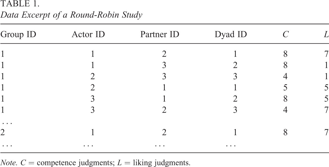
Note. C = competence judgments; L = liking judgments.
The univariate SRM is a mathematical model that can be used to analyze data stemming from the round-robin design. Consider pupil i’s judgment of pupil j. According to the SRM (see Kenny, 1994; Kenny, Kashy, & Cook, 2006, for an overview), i’s judgment consists of four components:

where μ is the overall mean across all judgments, gl is the group effect, α il is the actor effect of individual i in group l, β jl is the partner effect of individual j in group l, and γ ijl is the relationship effect. The group effect is a group-level effect indicating the average level of perceived competence in the group. The actor effect and the partner effect are individual-level effects. The actor effect indicates the extent to which i directs judgments toward others in general. For this example, it reflects how much i judges others as competent on average. The partner effect describes the extent to which a person is the target of a judgment, for example, how much j is judged to be competent by all other group members. The relationship effects are located at the dyadic level: They describe the unique component of the judgment after the actor- and partner-specific effects have been removed. In terms of the example, the relationship effect denotes i’s unique competence perception of j.
When analyzing SRM data, researchers typically focus on the estimation of the variance of the individual-level effects and the dyadic effects. In our example, the actor variance is a measure of how much perceivers differ in their average competence judgments. The target variance describes whether some targets are judged as more competent on average than other targets. The relationship variance describes whether dyads differ in their unique competence perceptions. One also estimates the covariance between the actor effects and the partner effects and the covariance between the relationship effects. The actor–partner covariance measures the extent to which the individual-level effects are correlated. In the competence example, a positive actor–partner covariance would indicate that pupils who judge others as competent on average are also judged to be more competent by other pupils on average. The relationship covariance describes the extent to which the relationship effects of the judgments of the same dyad (i.e.,
The Multivariate SRM
Imagine that you have assessed not only one but two (or even more) round-robin variables. In our example, pupils were not only asked to judge the competence of their fellow pupils but also how much they like them (see Table 1 again for a data excerpt). The multivariate SRM can also be used to analyze this multivariate round-robin data. The multivariate SRM results in far more parameters for estimation because one can estimate not only the univariate variance and covariance parameters just described (e.g., the actor variance of the competence judgments or the partner variance of the liking judgments) but also a number of additional cross-variable covariances.
For the level of the individual, there are four additional cross-variable covariance parameters for each pair of round-robin variables (e.g., liking and competence). The actor–actor covariance represents the association between the actor effects of the first variable and the actor effects of the second variable. In this example, a positive parameter would indicate that the more persons judge others as competent on average, the more they tend to like others on average. The partner–partner covariance describes the relationship between the partner effects of the two variables. A positive parameter in the example indicates that individuals who are judged to be competent on average are also liked more on average. The actor–partner covariance indexes the association between the actor effects on the first variable and the partner effects on the second variable. The parameter would be positive, for example, when persons who tend to perceive others as competent on average are also liked more on average. Finally, the partner–actor covariance measures the association of the partner effects of the first variable with the actor effects of the second variable. In this example, it measures whether being judged to be competent on average goes along with a stronger tendency to like others on average.
On the dyadic level, there are two cross-variable covariance parameters for a pair of two round-robin variables. The intraindividual relationship covariance measures the extent to which the unique effects of i's perceptions of j for the two variables are associated. In this instance, a positive parameter would indicate that i's unique competence perception of j goes along with i's unique liking of j. The interindividual relationship covariance, by contrast, represents the association of i's unique perception of j on one variable with j's unique perception of i on the other variable. Here, a positive parameter measures how much i's unique competence perception of j is related to j's unique liking of i. Finally, on the level of the group, one can estimate the group effect covariance for each pair of round-robin variables. In our example, a positive parameter would indicate that groups with higher average competence perceptions tend to have higher average liking judgments.
Estimation of the Multivariate SRM: A Likelihood Approach
Extending the univariate SRM to multiple variables involves estimating
Here, we suggest utilizing a likelihood approach instead as it will produce standard errors for all model parameters, and it is simple to use in the case of an arbitrary number of round-robin variables. Finally, undefined parameter estimates (e.g., negative variance estimates) are theoretically not possible, and strategies have been developed to avoid them when they occur during estimation (e.g., constrained estimation, see Demidenko, 2004, for an explanation of the different approaches).
We acknowledge that ML approaches have been suggested before in the literature (see e.g., Ackerman et al., 2011; Li & Loken, 2002; Li, 2006; Snijders & Kenny, 1999). Most of these approaches involve reformulating the SRM as an established statistical model and the use of standard software packages to estimate the models’ parameters. However, very often this results in time-consuming data preparation and of model definition that gets more error-prone as more round-robin variables are assessed. Snijders and Kenny (1999), for example, show that the univariate SRM can be transformed into a multilevel model and how established multilevel statistical software can be used to estimate this model. As we show below, the SRM can be considered a crossed random effects model in which the actor and partner effects as well as the relationship effects are correlated. In standard multilevel models, however, crossed random effects are assumed to be uncorrelated. Thus, to estimate the SRM (including all variance and covariance parameters) with multilevel software, a researcher must create a number of dummy variables and impose a number of constraints on the variance–covariance matrix of the model to estimate all SRM variance and covariance parameters. Similarly, developmental psychologists (see, e.g., Ackerman et al., 2011; Branje, van Lieshout, & van Aken, 2005; Buist, Reitz, & Dekovic, 2008) argued that the SRM can be analyzed with multiple-group structural equation models (SEM, see Kenny & Livi, 2009). Here, each judgment of a dyad is defined as the outcome of two latent factors and an error term. The two latent factors represent the actor effect and the partner effect, respectively, whereas the error term denotes the relationship effect. Each judgment is forced to load on these latent variables with a fixed factor loading of 1.0. Furthermore, a number of equality constraints for the variance and covariance parameters have to be imposed, so that they represent the correct univariate or multivariate variance and covariance parameters. We note that the SEM approach cannot be used in case of a single round-robin group.
To overcome the described slow and complex processes of data preparation and equality constraint definition, we suggest embedding the SRM into the mixed-model framework (e.g., Gill & Swartz, 2001; Nestler, 2016). Specifically, we will write the SRM as a crossed random effects model. This allows us to derive the variance–covariance matrix of the model and to use an established Fisher scoring algorithm to estimate the multivariate SRM parameters. We emphasize that the approach outlined here does not require a researcher to specify constraints on the variance–covariance matrix; it is thus much simpler than the multilevel approach or the multiple-group SEM approach. Furthermore, our approach allows the employment of ML or REML estimation for the SRM parameters. This is a more complex process in the multiple-group SEM approach, for example.
In the following, we will first outline the matrix formulation of the multivariate SRM. Thereafter, we will embed the model into the mixed-model framework and then describe the equations that can be used to implement a Fisher scoring algorithm for ML and REML estimation.
Matrix Formulation of the Multivariate SRM
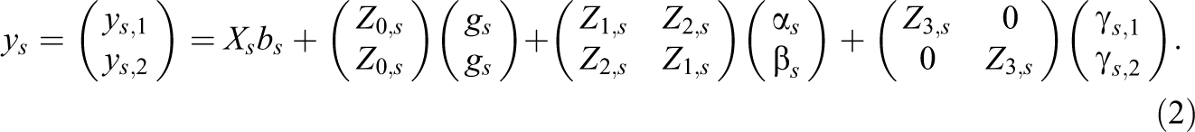
Before outlining the matrix formulation of the multivariate SRM, we start with the matrix formulation of the univariate SRM as defined in Equation 1. In the following, we assume that l round-robin groups had been assessed. In every group, m individuals were asked to fill out k round-robin measures. For each round-robin variable, l ⋅ m ⋅ (m − 1) judgments are then available. We note that the present framework is also applicable to unbalanced data situations (i.e., some group members made less than m judgments). However, to simplify the explanation, we assume a balanced data situation here. According to Gill and Swartz (2001), the vector of round-robin judgments concerning a single round-robin variable s can be written as
Here,
To formulate the multivariate SRM in matrix form, we assume that k round-robin variables have been assessed and that the judgments of each round-robin variable are arranged in accordance with the univariate matrix formulation. Stacking the single vectors above each other gives
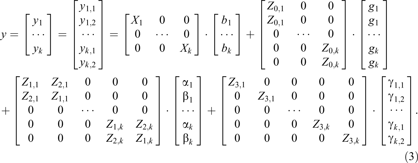
We note that Z 3,s for s ∈ 1, …, k is an identity matrix. When one substitutes ∊ for γ, then Equation 3 can also be written as

where u contains all group effects, actor effects, and partner effects, and Z is a block diagonal matrix containing the univariate design matrices
Covariance Matrix of the Judgment Vector
To this end, we assume that b is a fixed variable and that all round-robin parameters are normally distributed random variables that have an expectation of 0. The variance–covariance matrix of the group effects of the k round-robin variables is

where Il
is an l × l identity matrix and ⊗ is the Kronecker product. Covariance parameters of random effects sharing the same subscript refer to the univariate SRM covariance parameters, and covariance parameters sharing different subscripts refer to cross-variable covariance parameters.
The variance–covariance matrix of the actor and partner effects of the k round-robin variables is

where
The variance–covariance matrix of the relationship effects is
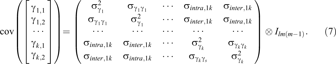
Here,
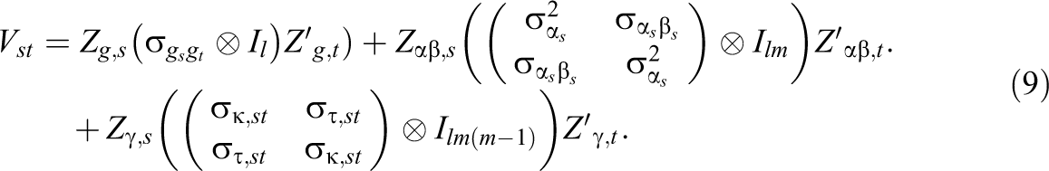
Given these definitions, the covariance matrix of the judgment vector V can be deduced. To this end, we will exploit that V has a block diagonal structure: It contains covariance matrices of the single round-robin measures on the main diagonal and the matrices containing the cross-variable covariance parameters in the off-diagonal elements. The variance–covariance matrix Vs of a single measure s is
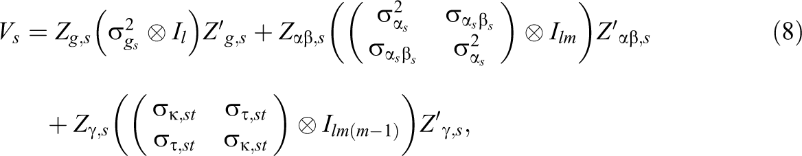
and an off-diagonal matrix block, Vst , containing the cross-variable covariance parameters of measures s and t, is
Here,

When we define a k × k—matrix Gi,j containing a 1 at position (i,j) and 0s otherwise, the covariance matrix V of y then is

ML and REML Estimation
Let

In the case of REML, one uses the restricted log-likelihood function

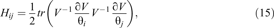
Differentiating these functions with respect to θ yields the following score equation (see McCulloch, Searle, & Neuhaus, 2004, for a proof):

for ML and

for REML. Here,
for ML and

for REML. Finally, to obtain estimates of the elements in b, ML and REML use the ML estimator of

where
In summary, likelihood estimation is based on embedding the SRM in the mixed-model framework. This presentation can overcome the problems that are associated with the earlier approaches that are used to estimate multivariate SRMs. In contrast to the ANOVA approach, for example, standard errors can be derived for both likelihood estimates. Furthermore, the approach suggested here does not require the process of defining equality constraints and can be used when the data of a single round-robin group are available.
Empirical Illustration
Kenny, Albright, Malloy, and Kashy (1994) report a round-robin experiment in which the group members of 29 round-robin groups (consisting of five to six individuals each, overall N = 159) were asked to judge how calm, sociable, likable, careful, relaxed, talkative, and responsible the other group members were. All judgments were assessed on 7-point Likert-type scales (ranging from 0 = not at all to 6 = very much). Here, we use three round-robin judgments, the calm, the relaxed, and the likable judgments, to illustrate the two likelihood methods and to compare their estimates with the estimates of the ANOVA method.
R (R Core Team, 2014) was used for all analysis. A Fisher scoring algorithm was implemented in R to obtain the two likelihood parameter estimates. ANOVA method estimates were computed using TripleR (Schönbrodt, Back, & Schmukle, 2017). As TripleR is able to compute only bivariate SRMs, ANOVA estimates were obtained by specifying three single bivariate SRMs. All R codes as well as the data can be downloaded from the Open Science Framework (https://osf.io/6b3dx/; the data can also be downloaded from http://davidakenny.net/srm/srmdata.htm; it is called FORMAT there).
Prior analysis of the data showed that the group variance parameters were low or negative for each of the single round-robin variables. We therefore decided to leave out the random group effects from the multivariate SRM model and to use a fixed-effects approach to control for the group structure in case of the two likelihood methods instead (Lüdtke et al., 2013; Nestler, 2016). The fixed-effects approach involved the creation of 29 dummy variables that code group membership. These dummy variables were then included as fixed effects in the multivariate SRM model. We emphasize that it is not possible to use the fixed-effects approach in case of the ANOVA method.
Table 2 shows the variance and covariance parameter estimates (and standard errors) obtained with the ML approach, the REML approach, and the ANOVA method. As can be seen, the estimates of the ANOVA method and the REML approach as well as the standard errors were very similar. Differences in the estimates of the variance and the covariance parameters occurred for the single-variable estimates when they were estimated with the ML method. A potential explanation of this finding is that the ML method considers the fixed effects during the variance component estimation (see Verbeke & Molenberghs, 2009).
Parameter Estimates (PE) and Standard Errors (SE) for the Illustrative Example
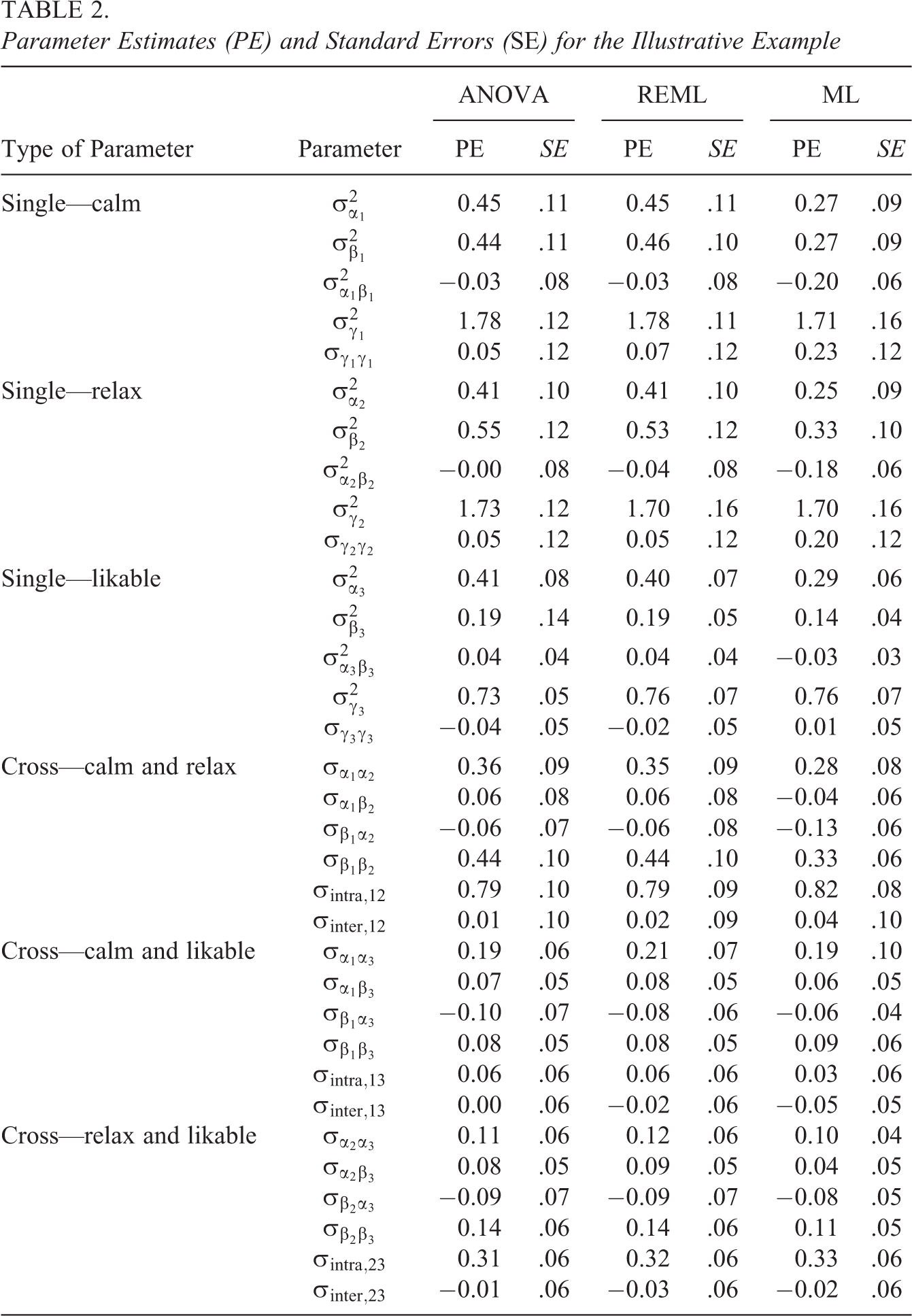
Concerning each of the single-variable estimates, the results of all three estimation methods show that there is considerable perceiver variance for all three measures. This indicates that actors differed in their average judgment of others as calm, relaxed, and likable. Similarly, targets differed in the amount they were judged as calm, relaxed, and likable on average as indicated by the magnitude of the target variance, although this parameter was greater for the calm and relax judgments compared with the likable judgments. Furthermore, the largest variance parameter for all three measures was the relationship variance. We note, however, that in the case of a single indicator per construct, relationship variance contains variation due to the unique perceptions of the dyad members but also measurement error. Finally, the actor–partner covariance and the relationship covariance were low for all measures: The correlation coefficients ranged between −.07 and .14.
With regard to the cross-variable covariance parameters, the results showed that the actor effects of the calm judgments and the actor effects of the relax judgments were highly correlated, r = .83. Participants who judged others as calm on average also judged others as relaxed on average. A similar result was obtained for the target effects: Participants who were judged as calm on average were also judged as relaxed on average, r = .89. These correlations were not as high for the likable judgments, rs ranged between .25 and .43. Finally, the intraindividual relationship covariance for the calm and relax judgments was also high, r = .42. i's unique calm perception of j went along with i's unique relax judgments of j. All other covariance parameters were lower or negligible.
Simulation Study
A small simulation study was done to compare the performance of the two likelihood methods and the ANOVA method in the estimation of the parameters of a bivariate SRM. We examined the performance under different conditions of the number of round-robin groups and the number of round-robin group members.
Population model and simulation conditions
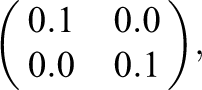
The population parameters were similar to the parameters found in the illustrative example. The variance–covariance matrix of the group effects was set to
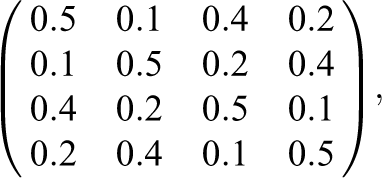
the variance–covariance matrix for the individual-level effects was set to
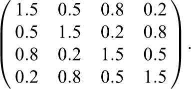
and the variance–covariance matrix for the dyad-level effects was set to
We manipulated the number of round-robin groups and the number of round-robin group members. The number of groups was either l = 10 or l = 20, and a round-robin group contained either m = 5 or m = 10 round-robin group members. The R package version 1.0.6 mvtnorm (Genz et al., 2017) was used to generate the population and to draw 500 samples from the population for each of the four simulation conditions.
Dependent measures
The relative bias (RB) of the parameter estimates, the root mean square error (RMSE), and the coverage rate (CR) were used to evaluate the performance of the three estimation approaches (Lüdtke et al., 2013). The RB was computed by taking the average of the estimates of a parameter in a simulation condition, taking the difference between this average and the true parameter, and dividing the difference by the true parameter (i.e.,
Results
Tables 3 through 5 present the results of the simulation study. For each parameter group (e.g., single-measure variance estimates), we averaged the resulting RB, RMSE, or CR for each parameter belonging to the group (e.g., RB of actor variance and RB of partner variance) to economically present our findings. As can be seen in Table 3, all three estimators yielded acceptable parameter estimates in all simulation conditions with the two likelihood methods having slightly smaller average RBs for the single-variable covariance parameters and the cross-variable covariance parameters when the number of round-robin groups and the number of round-robin group members were small. For the variance parameters, the RBs for the three estimation methods were very similar in all of the simulation conditions. Largely, identical results were obtained for the RMSE. It was slightly lower for the two likelihood methods in case of the covariance parameters when the number of round-robin groups as well as the group size was small and they were very similar across the three methods in case of the variance parameters. The CRs of the two likelihood methods were closer to nominal values for most parameters compared to the ANOVA method in conditions were the group size was n = 5. When the group size was large, n = 10, CRs for the three estimators were almost identical and close to nominal values. Altogether, these results support the usefulness of the likelihood estimators to model multivariate SRM data. They are also consistent with earlier research, showing that the higher the number of round-robin group members (irrespective of the number of round-robin groups), the more accurate and the more efficient are the SRM parameter estimates (e.g., Lüdtke et al., 2013; Nestler, 2016).
Average Relative Bias in Percent of Single-Variable Social Relations Model Parameters and Cross-Variable Parameters Depending on the Estimator, the Number of Group Members, and the Number of Groups

Note. ANOVA = analysis of variance; ML = maximum likelihood; REML = restricted maximum likelihood approach.
Root Mean Square Error of Single-Variable Social Relations Model Parameters and Cross-Variable Parameters Depending on the Estimator, the Number of Group Members, and the Number of Groups
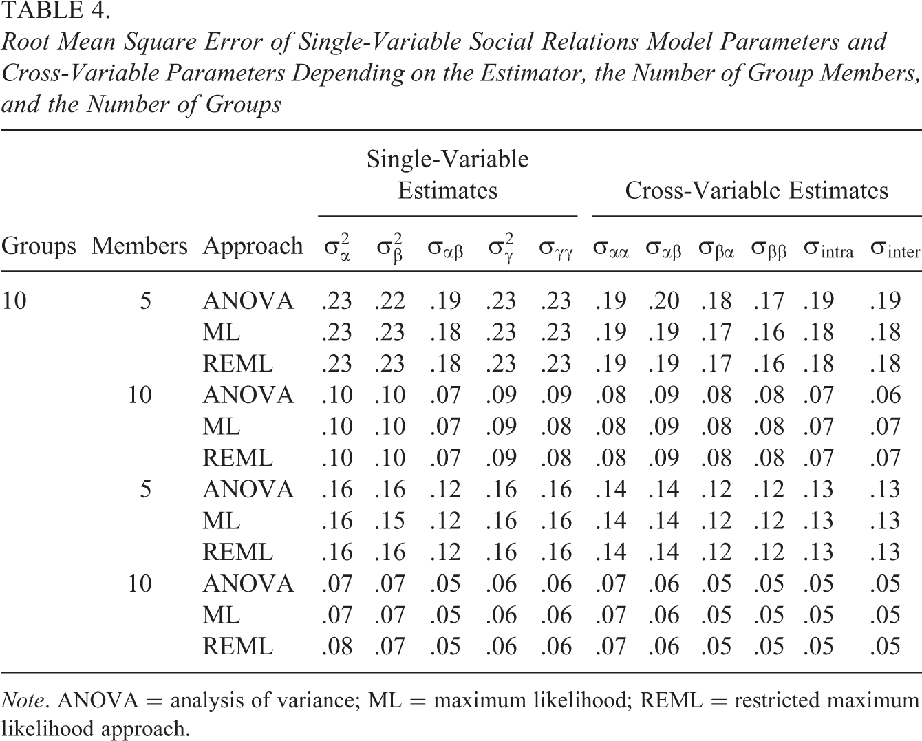
Note. ANOVA = analysis of variance; ML = maximum likelihood; REML = restricted maximum likelihood approach.
Coverage Rates of Social Relations Model Parameters and Cross-Variable Parameters Depending on the Estimator, the Number of Group Members, and the Number of Groups
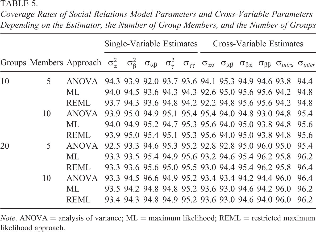
Note. ANOVA = analysis of variance; ML = maximum likelihood; REML = restricted maximum likelihood approach.
Discussion
The aim of the present article was to introduce an ML estimator and an REML estimator for the parameters of a multivariate SRM. The basis for deriving the two likelihood estimation methods was to embed the multivariate SRM into the framework of (linear) mixed models. This presentation has a number of advantages in comparison with the earlier approaches used to analyze multivariate round-robin data: First, both approaches can be used in case of an arbitrary number of k round-robin variables, a single round-robin group, and without running through a tedious process of defining parameter equality constraints (as in the case of a multiple-group SEM or a multilevel approach). Second, standard errors can be simply derived, and third, an established significance test for the covariance components is available. Finally, although we did not show this here, the influence of explanatory variables for the SRM-specific effects can be easily investigated (see Gill & Swartz, 2001). Overall, therefore, these arguments and the findings of the simulation study suggest the use of the two likelihood approaches instead of the ANOVA approach.
The model and methods suggested here offer some interesting analysis options for applied research as they allow the relating of the SRM components of different round-robin measures to each other. This may be interesting in the case of educational psychology, for example, where competence judgments concerning different disciplines (e.g., math, language, and art) could be simultaneously analyzed or where the correspondence between the SRM components in competence and interpersonal variables such as liking can be investigated. Furthermore, estimation of the multivariate SRM is also important from a statistical perspective, as the multivariate SRM is a saturated model. Hence, the fit of this model can be used as a benchmark to evaluate the fit of other models. Nestler, Geukes, Hutteman, and Back (in press), for example, suggest the model be utilized to evaluate the fit of a growth model that was selected to analyze longitudinal SRM data.
The present approach could also be used for further methodological research. One issue that we deem important is to extend the present approach to multiple indicators of a round-robin construct. For example, a researcher has assessed liking as well as competence with three round-robin indicators and not just one indicator. The algorithm presented here allows the researcher to estimate such a multiple indicator–multivariate SRM with the restriction that the factor loadings of the indicators are one. As this assumption is unrealistic in applied contexts, we believe that it is in interesting task for future research to establish a more realistic mixed-model approach (see Rabe-Hesketh & Skrondal, 2004, for such a possible extension). Alternatively, a multiple-group SEM approach might be used, at least when more than one round-robin group is available. However, the model definition for the respective SEM model has yet to be defined.
Another task for future research is to increase the practicability of the estimation algorithm used for the two likelihood methods. Here, we used a Fisher scoring approach that involves the inversion of the variance–covariance matrix V. As V has a very complex structure (see Equation 10), we employed a standard procedure in R to compute the inverse of V. However, when V has a large dimension, this procedure results in long computation times. An alternative approach may be to use a profile-likelihood approach for parameter estimation (e.g., Pawitan, 2001). The R package xxM implements such an approach to estimate the parameters of univariate SRMs with multiple indicators (see Mehta, 2013). Alternatively, one may use a Bayesian estimation approach (see below).
In our simulation study, the two likelihood methods performed equally well with regard to parameter bias, RMSE, and CR. Hence, another interesting task for future research would be to investigate the conditions in which the performance of the two likelihood methods will differ. Earlier simulation research, for example, showed that REML outperforms ML the greater the number of fixed effects included in the model (see also the illustrative example). It would be interesting to examine whether this finding replicates in the case of multivariate SRMs. Another objective for future research would be to compare the two likelihood methods to a Bayesian approach, for example, where these is a small number of round-robin group members. However, until now the Bayesian approach has been implemented for univariate SRMs only (see Lüdtke et al., 2013). It would be prudent to expand this research to the multivariate case in the first place.
In sum, the present article showed how the parameters of a multivariate SRM can be estimated with an ML approach and an REML approach. The illustrative example and the results of a small simulation study showed that the two estimators provide consistent and efficient parameter estimates and that the model can be used to examine a number of interesting research questions.
Footnotes
Author’s Note
This article is dedicated to Irmgard Laufer.
Acknowledgment
I am grateful to Sarah Humberg for very helpful comments on an earlier version of the manuscript.
Declaration of Conflicting Interests
The author(s) declared no potential conflicts of interest with respect to the research, authorship, and/or publication of this article.
Funding
The author(s) received no financial support for the research, authorship, and/or publication of this article.