
Abstract
Widespread availability of rich educational databases facilitates the use of conditioning strategies to estimate causal effects with nonexperimental data. With dozens, hundreds, or more potential predictors, variable selection can be useful for practical reasons related to communicating results and for statistical reasons related to improving the efficiency of estimators. Background knowledge should take precedence in deciding which variables to retain. However, with many potential predictors, theory may be weak, such that functional form relationships are likely to be unknown. In this article, I propose a nonparametric method for data-driven variable selection based on permutation testing with conditional random forest variable importance. The algorithm automatically handles nonlinear relationships and interactions in its naive implementation. Through a series of Monte Carlo simulation studies and a case study with Early Childhood Longitudinal Study–K data, I find that the method performs well across a variety of scenarios where other methods fail.
Keywords
1. Introduction
Widespread availability of high-quality educational databases such as the Early Childhood Longitudinal Study (ECLS-K; Tourangeau, Nord, Lé, Pollack, & Atkins-Burnett, 2006) has made it easier for educational researchers to search for answers to causal research questions with nonrandomized data through conditioning strategies. To identify an average causal effect with observational data through a conditioning strategy, such as regression estimation or propensity score analysis, one must assume that the potential outcomes are independent of the assignment mechanism, conditional on the observed pretreatment variables,
From a practical perspective, a researcher using a large database may wish to winnow down the set of predictors from the dozens, hundreds, or thousands available to a more manageable number to (a) facilitate interpretation and communication of results, 1 (b) allow parametric models to be stably fit, or (c) allow nonparametric algorithms to converge in a reasonable amount of time. From a statistical perspective, the indiscriminate inclusion of conditioning variables that are not associated with the potential outcomes will decrease the efficiency of causal effect estimators, even if ignorability is satisfied (Hahn, 1996, 2004). Substantive knowledge should play a prominent role in guiding which variables should be retained for conditioning, with an eye toward selecting multiple variables from heterogeneous domains (Steiner, Cook, Li, & Clark, 2015). However, especially when the number of candidate variables is large and/or the theory is weak, data-driven approaches may serve as a useful complement to theory-based variable selection.
In this article, I develop a computationally feasible algorithm for nonparametric conditional independence testing that is particularly useful for variable selection in the context of estimating causal effects by conditioning. The algorithm, implemented in R package
2. Theoretical Framework
Let

To estimate an average treatment effect with a conditioning strategy, one or both of
It has been shown both analytically (Battacharya & Vogt, 2007) and through simulation (Austin, Grootendorst, & Anderseon, 2007; Brookhart et al., 2006) that conditioning on treatment-only predictors (i.e., instrumental variables [IVs]) can decrease the efficiency of propensity score-based estimators, while conditioning on outcome-only predictors can increase efficiency. Furthermore, conditioning on an IV or a collider variable can amplify bias (Battacharya & Vogt, 2007; Pearl, 2010; Steiner & Kim, 2016; Wooldridge, 2009). Although de Luna et al. (2011) proposed a number of target subsets for variable selection, I focus on the subset they refer to as

where
If ignorability holds with
As an example, consider the graphical models for the potential outcomes,

Directed acyclic graphs for potential outcomes Y 0 and Y 1.
3. Random Forests and Variable Importance
The
3.1. Regression Trees
A regression tree is an algorithmic tool invented by Breiman, Friedman, Olshen, and Stone (1984), which models the relationship between a continuous outcome variable (

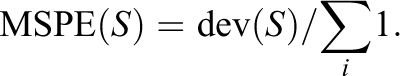
The adequacy of a regression tree fit may be measured by the deviance, defined for tree

At each iteration, the tree-fitting algorithm considers every possible split on every variable, and the single split that results in the largest decrease in deviance is selected. If left unchecked, regression trees will continue to split until each terminal node contains only one unit, yielding a perfect fit to the data. A typical approach to prevent overfitting is to fit a complex tree and then “prune” it by dropping nodes according to a regularized solution based on adding a term to the deviance that penalizes additional nodes (see, e.g., Hastie, Tibshirani, & Friedman, 2009, or Venables & Ripley, 2002, for details). The value of the penalty term coefficient is typically chosen by cross-validation (see Appendix A in the online version of the journal for an example in which regression trees are applied to ECLS-K data).
3.2. Random Forests and Variable Importance
A single regression tree yields a rather noisy fit to the data. That is, minor changes to the data can result in drastic changes to the predicted values for certain units. Bagging, short for bootstrap aggregating, helps to reduce the variability of tree-based predictions by averaging over a collection of fits produced on bootstrap samples of the data. A random forest (RF) is a collection of
Breiman (2001) introduced the permutation measure of variable importance. For each predictor
Let
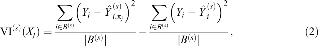
where

The importance method described in Equations (2) and (3) will be referred to as traditional RF permutation importance. A problematic feature of the traditional permutation scheme is that variables may attain a high level of importance either for their relationship with the outcome
3.3. Conditional Permutation Importance
Strobl, Boulesteix, Kneib, Augustin, and Zeileis (2008) proposed conditional permutation importance to disentangle marginal and conditional relations. For each regression tree in the random forest and for a given predictor variable,
With more than a handful of predictors, sparsity due to the “curse of dimensionality” renders the exact approach implausible. In place of exact conditioning, one could condition on any balancing score (cf. Rosenbaum & Rubin, 1983) for the target predictor. For example, if the target predictor (i.e., the one to be permuted) is dichotomous, it may be permuted within strata based on the propensity score estimated by regressing the target predictor on the remaining predictors. For continuous or multicategory variables, generalized versions of the propensity score could be used (e.g., Fong, Hazlett, & Imai, 2018). The approach suggested by Strobl et al. (2008) is to permute within subgroups based on the random forest regression tree splits. This latter approach has the benefit of being fully nonparametric.
4. Nonparametric Conditional Independence Testing
A test of conditional independence, as opposed to one that fails to distinguish between marginal and conditional association, is particularly important for variable selection in causal inference applications. Consider the example depicted in Figure 2, where
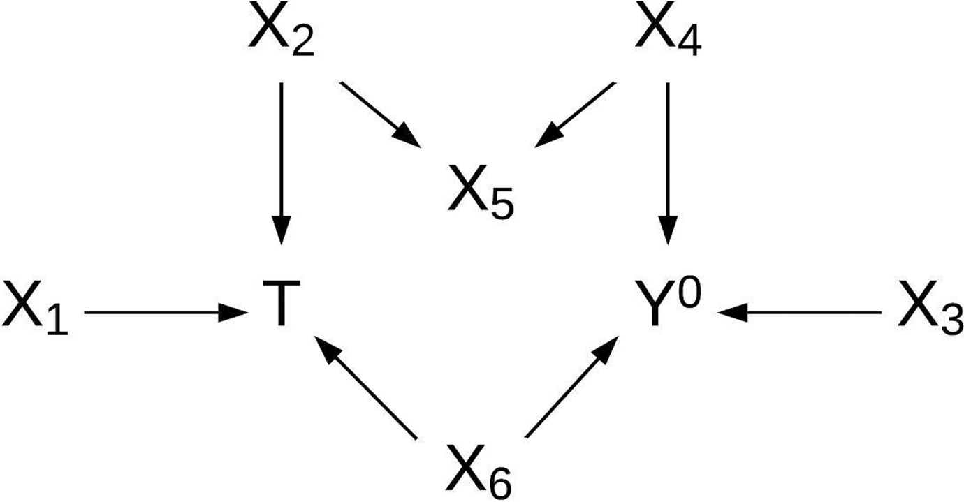
If tests of marginal, rather than conditional, independence are used to determine X 0 with this directed acyclic graph, X 1 and X 5 are incorrectly retained.
4.1. Permutation Testing With RF Permutation Importance
Permutation testing provides a useful framework for nonparametrically testing individual variables based on RF importance measures. Rodenburg et al. (2008) used permutation of traditional RF permutation importance for variable selection, and Altmann, Toloşi, Sander, and Lengauer (2010) summarized the approach, which can be described in four steps.
The permutation approach operationalized in Steps 1 through 4 does not provide a test of conditional dependence for each predictor variable. There are two potential solutions to correct the procedure so that it provides tests of conditional independence between predictors and outcome, as desired. The first, proposed by Hapfelmeir and Ulm (2013), is to modify Steps 2 and 3 as follows, where
This modification requires that
I use this latter approach and build up conditional RF permutation importance as follows: Fit a random forest to the un-permuted data with n
tree trees and compute OOB MSPE. For each tree in the random forest, For Let The overall conditional RF importance for
The calculation of conditional RF importance requires significantly more computational time than the calculation of traditional RF importance. To reduce overall runtime, permutation testing with conditional RF importance is implemented only after first dropping predictors based on permutation testing with traditional RF importance. In this way, predictors that have no marginal association with the potential outcomes are dropped quickly, thereby reducing the dimension of the space over which conditional RF importance is run.
5. Simulation Studies
To my knowledge, the only other nonparametric approaches that have been studied for conditional independence testing within the
5.1. Variable Selection and Effect Estimation
Simulation studies were planned for four DGPs, each based on 100 replications, to probe the performance of the conditional RF importance permutation approach (RFC) relative to three other methods for high-dimensional variable selection: traditional RF importance under permutation (RFT), GBNs run in package
First, propensity score analysis was run with propensity scores estimated by generalized boosted regression models via package
For variable selection, performance was measured by the proportion of replications for which variables in the target set,
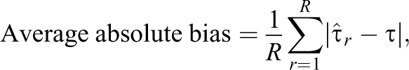
where
5.2. Data Generation
The DGPs for
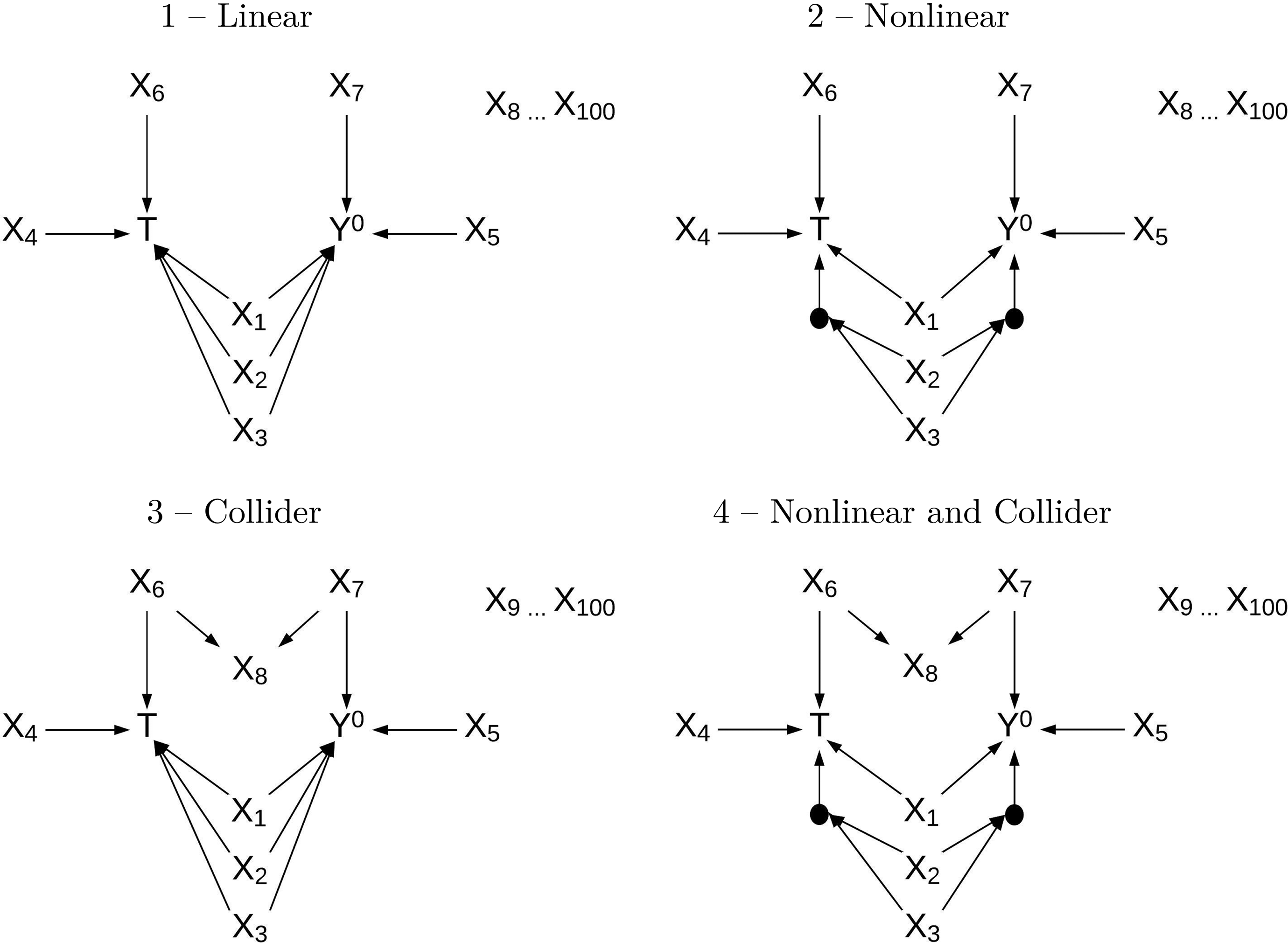
Data generating processes for Y 0 for the four simulation studies. Data generation for Y 1 is identical with the exception of a constant treatment effect.
The nonlinear DGP was identical with the exception that variables
Motivating considerations for the four DGPs are related to expected differences in performance across the methods with respect to variable selection and estimation accuracy and precision. Considerations for variable selection: All methods are expected to perform well when the DGP is linear. Methods based on RF importance should outperform GBNs and CSH in correctly identifying variables involved in nonlinear relationships with the potential outcomes. GBNs use mutual information based on Gaussian log likelihoods for conditional independence testing, so there is an implicit assumption that relationships between variables are linear. The CSH algorithm is based on the discrete version of mutual information, which does not assume linearity. However, because continuous variables must be discretized, information loss will likely result in less sensitivity to detect relationships that will be especially noticeable for small to moderate sample sizes. RFT, which is the only method of the four that fails to distinguish marginal from conditional independence, will fail to eliminate collider variables because they are marginally associated with the potential outcomes.
Considerations for estimation precision and accuracy: IVs and noise variables decrease precision of estimation when conditioned on; thus, all methods are expected to perform more poorly with respect to finite sample bias and efficiency when all 100 predictors are included, relative to when only the target set Conditioning on an IV or a collider variable has the potential to amplify bias; thus, large biases are expected in cases where the incorrect retention of an instrument or collider co-occurs with the incorrect omission of key confounding variables.
5.3. Results: Variable Selection
Variable selection results are shown in Figure 4. The bars represent the proportion of 100 replications that included each variable from
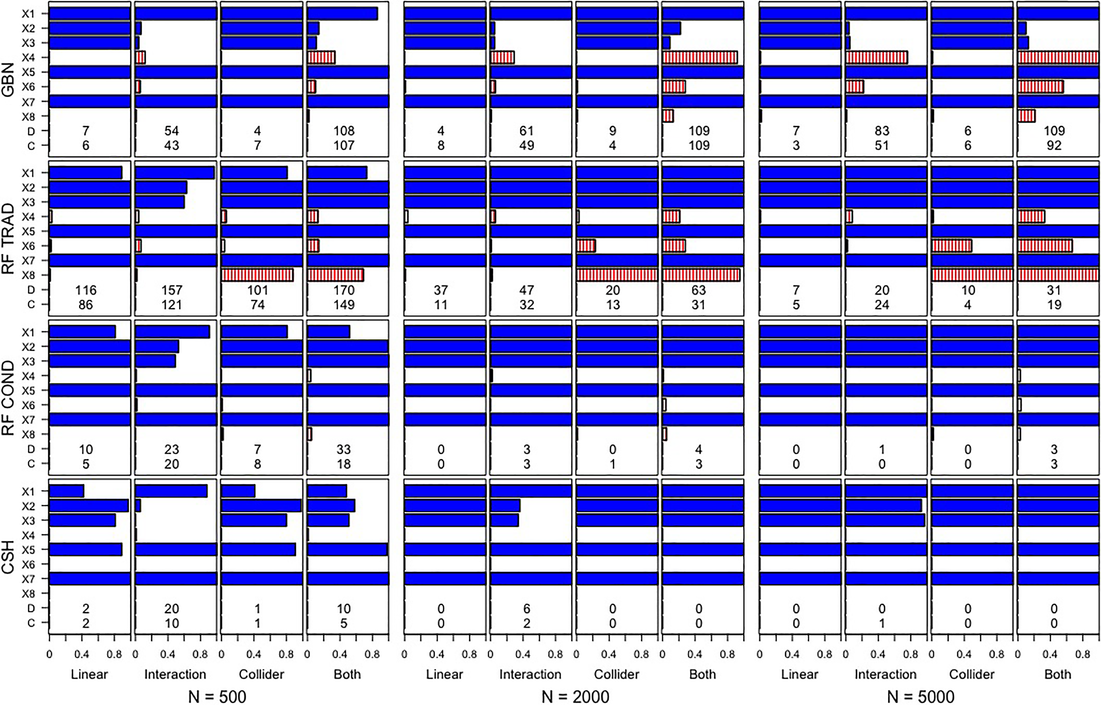
Bars represent Monte Carlo simulation study results on the proportion of 100 replications each variable was retained. Solid bars denote variables that were correctly retained (because they are in X Y ); striped bars denote variables that were incorrectly retained. For each cell, rows labeled D and C give the number of dichotomous and continuous noise variables incorrectly retained, respectively. GBN = Gaussian Bayesian networks; RF TRAD = traditional RF permutation importance under permutation; RF COND = conditional RF permutation importance under permutation; CSH = discrete Bayesian networks.
The overall patterns of results are largely as expected. First, note that GBN performs remarkably well when relationships are linear (either with or without a collider variable) and very poorly when relationships are nonlinear. For the nonlinear DGPs, IVs
The RFC method performed well across all scenarios. For the moderate and large sample size conditions, with
5.4. Results: Estimation
In addition to variables selected by GBN, RFT, RFC, and CSH, the cases of no variable selection (ALL) and correct selection of the target set

Each point represents the simulation-based average absolute bias for a given sample size, variable selection method, and estimation method. Variable selection methods: ALL = no variable selection; GBN = Gaussian Bayesian networks; RFT = traditional RF permutation importance under permutation; RFC = conditional RF permutation importance under permutation; CSH = discrete Bayesian networks; XY = correct selection of the variables in X Y .

Each point represents the simulation standard deviation for a given sample size, variable selection method, and estimation method. ALL = no variable selection; GBN = Gaussian Bayesian networks; RFT = traditional RF permutation importance under permutation; RFC = conditional RF permutation importance under permutation; CSH = discrete Bayesian networks; XY = correct selection of the variables in X Y .
In every cell of the design and across all estimation methods, the absolute bias based on conditioning on all 100 predictors (ALL) was larger than the bias due to conditioning only on the target set,
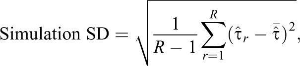
The variability of estimators after variable selection, as measured by simulation SD, contributed relatively little to the RMSE; nevertheless, there were some trends with respect to variability. After variable selection with CSH, nonparametric estimators (i.e., BART, TMLE with BART, and propensity score analysis with GBM) were associated with larger variances. As an example, consider the interaction DGP at N = 5,000. For that cell of the design, 91 of the 100 replications led to estimates between 0.4 and 0.6 (the true value was 0.5), but the remaining 9 estimates were larger than 1.0. In those 9 cases, the CSH procedure had resulted in the incorrect omission of
6. Case Study
In this section, variable selection methods are applied to ECLS-K data to estimate the average causal effect of exposure to special education services on math achievement in fifth grade. The data set, which is described in greater detail in Keller and Tipton (2016), includes variables motivated by Morgan, Frisco, Farkas, and Hibel (2010) who examined the effect of student exposure to special education services on later social and academic outcomes. There are 429 exposed cases and 6,933 comparison cases; the outcome variable and 34 potential predictor variables are summarized in Table A1 in the online version of the journal. Note that these analyses are illustrative; resultant estimates should not be interpreted as robust estimates of the causal effect.
6.1. Results: Variable Selection
Variable selection results are shown in Table 1. Of 34 potential predictors, 12 were retained by GBN, 10 by RFT, 8 by RFC, and 5 by CSH. The five variables selected by CSH were also selected by all other methods. Because these data were not simulated, the true value of the treatment effect is not known. Nevertheless, patterns in the variable selection results correspond with expectations based on theory and simulation results. For example, kindergarten reading score (RIRT) was dropped by all methods except RFT. Recall that RFT is the only method of the four that fails to discriminate between conditional and marginal dependence. The marginal linear relationship between RIRT and kindergarten math score (MIRT) is quite strong, with an estimated Pearson correlation of .71. It is plausible that the impact of RIRT on the outcome, fifth-grade math score, although marginally very strong, was conditionally weak after accounting for MIRT, which would explain why it was dropped by the other algorithms. Another example involves P1FIRKDG (an indicator for first time in kindergarten) and P1AGEENT (child’s age when starting kindergarten); both were selected by the RF procedures but not by GBN nor by CSH. Based on exploratory linear regression modeling, P1FIRKDG and P1AGEENT were found to be involved in highly significant and strong two-way interactions. The forest-based methods may have picked up on these variables because of their strong nonlinear relationships with the outcome.
Subset of ECLS-K Variables Retained by at Least One Variable Selection Method
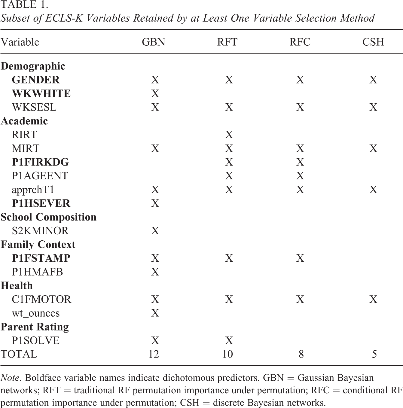
Note. Boldface variable names indicate dichotomous predictors. GBN = Gaussian Bayesian networks; RFT = traditional RF permutation importance under permutation; RFC = conditional RF permutation importance under permutation; CSH = discrete Bayesian networks.
6.2. Results: Estimation
Average causal effect estimates and 95% confidence intervals are displayed in Figure 7. For GBM and CBPS, 95% confidence intervals are based on sandwich standard errors from package

ECLS-K case study results including average treatment effect estimates (points with cross-hairs) and 95% confidence intervals for the effect of special education services on math achievement in fifth grade. For effect estimation: GBM = propensity score analysis via generalized boosted modeling; CPBS = propensity score analysis via covariate balancing propensity score; TMLE = targeted maximum likelihood; BART = Bayesian additive regression trees. For variable selection: ALL = no variable selection; GBN = Gaussian Bayesian networks; RFT = permutation testing with traditional RF permutation importance; RFC = permutation testing with conditional RF permutation importance; CSH = discrete Bayesian networks; ECLS-K Early = Childhood Longitudinal Study.
Adjusting for all 34 covariates drastically and significantly reduced the estimated average effect to between −5.4 and −1.8, depending on the estimation method, with three of the four 95% confidence intervals excluding zero and, thus, still suggesting a significant negative impact of exposure to special education services on fifth-grade math achievement. Conditioning only on variables selected by GBN gave estimates between −5.0 and −3.6, also with three of the four intervals excluding zero. Conditioning on variables selected by CSH yielded estimates between −6.4 and −3.8, with all intervals excluding zero. The use of RFT lead to estimates between −2.4 and 0.1, with only one interval that excluded zero. Estimates based on RFC were between −3.8 and −1.6 with two of the four intervals excluding zero.
There are no randomized experimental results to use as benchmarks for comparison because of obvious ethical issues. Without recourse to the true causal effect, it is not possible to say which methods were most unbiased. Nevertheless, it is interesting to note that the two RF-based methods tended to produce estimates closer to zero than any of the other methods including conditioning on all 34 available predictors.
7. Discussion
By using conditional RF importance in a permutation testing approach, one gets the best of both worlds: (a) a nonparametric variable selection algorithm that automatically handles nonlinear relationships and (b) one that tests the null hypothesis of conditional independence that is typically desired for causal applications. RF permutation methods were compared with GBNs and discrete Bayesian networks (CSH) through simulation and in a case study. Unlike GBN, which may fail to detect nonlinear relationships no matter the sample size, CSH is model free and has ideal properties in the limit. What the simulation results underscore, however, is that for small to moderate sample sizes, RF-based algorithms can be more powerful, especially for detecting nonlinear relationships.
A general limitation with any variable selection method is related to the potential to drop weak confounding variables due to lack of sensitivity. This could be problematic in a situation in which there are many very weak confounders that, in aggregate, reduce a nontrivial amount of bias but individually are too weak to be detected. The simulations show that sensitivity increases as sample size increases, as expected. Nevertheless, future work that more specifically addresses sample size and effect size considerations would be useful.
There are two limitations associated specifically with RF permutation methods for variable selection. First, RFT and RFC take more time to run than GBN or CSH because permutation approaches are computationally expensive. Second, as is typically the case with nonparametric methods, if parametric and functional form assumptions are tenable, methods such as GBN that capitalize on those assumptions will have slightly better finite-sample properties. This second point is not a strong limitation, however, because data-driven variable selection, especially with high-dimensional data, is typically used precisely because there is no strong theory regarding how variables are related. Furthermore, the consequences of incorrectly making strong functional form assumptions can be dire, as seen in the biases associated with GBN in nonlinear scenarios.
As expected, RFC correctly eliminated collider variables and IVs that were incorrectly retained by RFT. The implications for bias, however, were generally modest, with relatively small gains in accuracy for RFC over RFT. From a causal perspective, the inclusion of a collider variable (like
With respect to the simulation SDs, shown in Figure 6, the simulation SDs appear to be tied to the variable selection results via the bias; higher variability occurs in tandem with higher bias and poorer variable selection accuracy. This raises questions about the need to account for variability due to the variable selection procedure in confidence intervals and standard errors. The most straightforward methods to do so involve resampling, which, unfortunately, compounds computational time.
Note that RFC is an explicit method for variable selection. That is, the RFC procedure is designed be used as a preprocessing step to select important variables for further analyses. This is in contrast to methods that select variables implicity by upweighting important variables and downweighting unimportant ones on the fly. Some examples of methods that do implicit variable selection are penalized versions of regression such as ridge, lasso, and elastic net (Hastie et al., 2009), and all methods based on regression trees, which, as described in Appendix A in the online version of the journal, only make use of variables that maximize prediction when splitting. BART and GBM are both based on regression trees and, therefore, do variable selection implicitly by only splitting on important variables. Nevertheless, the use of RFT and RFC for variable selection always led to less bias than using the full set of variables with BART and GBM for the simulated data sets examined herein. As is the case with any simulation study, however, it is not appropriate to make strong generalizations to data scenarios that are very different.
Expert substantive knowledge and results from prior literature should take precedence in guiding the selection of important conditioning variables in an attempt to satisfy the ignorability assumption. However, there are bound to be variables, a large majority in some cases, for which the theory is weak. It is precisely for variables for which the theory is weak that questions about conditional independence and functional form relationships are likely to be unanswered. Simulation results discussed herein confirm that dropping IVs, colliders, and spurious noise variables prior to causal effect estimation improved finite sample behavior. The RFC algorithm performed well in both an absolute sense and relative to other methods for data-driven variable selection across a variety of conditions. Importantly, no tuning is required; RFC handles nonlinear relationships and interactions in its naive implementation.
Supplemental Material
Supplemental Material, DS_10.3102_1076998619872001 - Variable Selection for Causal Effect Estimation: Nonparametric Conditional Independence Testing With Random Forests
Supplemental Material, DS_10.3102_1076998619872001 for Variable Selection for Causal Effect Estimation: Nonparametric Conditional Independence Testing With Random Forests by Bryan Keller in Journal of Educational and Behavioral Statistics
Footnotes
Acknowledgments
I thank Xavier de Luna, Jenny Häggström, and Peter Steiner for helpful discussion on an earlier draft of this article.
Declaration of Conflicting Interests
The author(s) declared no potential conflicts of interest with respect to the research, authorship, and/or publication of this article.
Funding
The author(s) received no financial support for the research, authorship, and/or publication of this article.
Notes
References
Supplementary Material
Please find the following supplemental material available below.
For Open Access articles published under a Creative Commons License, all supplemental material carries the same license as the article it is associated with.
For non-Open Access articles published, all supplemental material carries a non-exclusive license, and permission requests for re-use of supplemental material or any part of supplemental material shall be sent directly to the copyright owner as specified in the copyright notice associated with the article.