
Abstract
With the widespread use of computers in modern assessment, online calibration has become increasingly popular as a way of replenishing an item pool. The present study discusses online calibration strategies for a joint model of responses and response times. The study proposes likelihood inference methods for item paramter estimation and evaluates their performance along with optimal sampling procedures. An extensive simulation study indicates that the proposed online calibration strategies perform well with relatively small samples (e.g., 500∼800 examinees). The analysis of estimated parameters suggests that response time information can be used to improve the recovery of the response model parameters. Among a number of sampling methods investigated, A-optimal sampling was found most advantageous when the item parameters were weakly correlated. When the parameters were strongly correlated, D-optimal sampling tended to achieve the most accurate parameter recovery. The study provides guidelines for deciding sampling design under a specific goal of online calibration given the characteristics of field-testing items.
Keywords
1. Introduction
Many testing programs nowadays make use of large item pools to create multiple parallel test forms or to continuously administer tests over a targeted population. For example, computerized adaptive testing (CAT) requires an extensive item pool to accommodate a variety of content areas and cognitive attributes. When an item pool is used continuously over a span of time, however, some items become obsolete, overexposed, or dysfunctional. These items need to be replaced by new items in a timely manner in order to preserve the quality of the item pool and of the prospective tests.
There have been broadly two approaches for replenishing an item pool. The conventional method is to embed new items in operational assessment and calibrate them together after field-testing is completed. This process is followed by a linking step that places the estimated parameter values on the scale of operational item parameters. The alternative method is online calibration, which calibrates items in real time during operational assessment. Online calibration is particularly favored when an assessment is performed using computers. With the aid of computers, it can achieve higher efficiency in replenishing an item pool as well as greater flexibility in designing a field-testing plan.
The current literature on online calibration is mostly centered on estimation methods (e.g., Ban, Hanson, Wang, Yi, & Harris, 2001; Ban, Hanson, Yi, & Harris, 2002; Segall, 2003) or sampling procedures (e.g., Berger, 1991, 1992, 1994; Buyske, 2005; Chang & Lu, 2010; Jones & Jin, 1994; Ren, van der Linden, & Diao, 2017; Stocking, 1988; van der Linden, 1988; van der Linden & Ren, 2014). More recently presented studies have considered contemporary measurement models such as multidimensional item response models and cognitive diagnostic models (e.g., P. Chen, 2017; P. Chen & Wang, 2016; P. Chen, Wang, Xin, & Chang, 2017; P. Chen, Xin, Wang, & Chang, 2012; Zheng, 2016).
Notice that the existing studies drew mainly on response data and paid no attention to time data that can be readily accessed in any computerized tests. Prior research suggests that response times can contain useful information about examinees’ cognitive processes and item characteristics (e.g., Klein Entink, Kuhn, Hornke, & Fox, 2009). Furthermore, they can help improve the precision of estimation of the response model parameters (van der Linden, Klein Entink, & Fox, 2010). Not only can they provide collateral information for analyzing response data, response times have also become increasingly popular in today’s testing and used in various sectors of psychometric applications. For instance, response time information has been used in assembling tests (van der Linden, 2011), selecting items in CAT (Fan, Wang, Chang, & Douglas, 2012; van der Linden, 2008), detecting aberrant response behaviors (Fox & Marianti, 2017; Marianti, Fox, Avetisyan, Veldkamp, & Tijmstra, 2014; van der Linden & Guo, 2008; van der Linden & van Krimpen-Stoop, 2003), controlling test administration time (van der Linden, 2009; van der Linden, Scrams, & Schnipke, 1999), to name a few. Clearly, it is of critical importance to procure accurate parameter estimates of the response-time models in these applications in order to make informed decisions and appropriate inferences.
The purpose of this article is to present and evaluate online calibration strategies for a joint model of responses and response times. The procedures are developed within the hierarchical framework (van der Linden, 2007) that has been widely used in the literature and in practice. In this study, we propose efficient estimators for the hierarchical framework that can be applied to online calibration settings. Note that there exist estimation routines developed for the hierarchical framework (e.g., Fox, Klein Entink, & van der Linden, 2007; Klein Entink, Fox, & van der Linden, 2009; van der Linden, 2006, 2007). These procedures, however, are based on Markov chain Monte Carlo algorithm and are hardly viable in online calibration due to computational intensity. The procedures developed in this study, by contrast, are grounded on likelihood inference and can be applied to computationally demanding situations such as online calibration and large-scale data analysis.
The present approach is in the similar vein with Glas and van der Linden’s (2010) approach, which applied marginal likelihood inference to evaluate abnormality in items (e.g., differential item functioning, local dependence). While the preceding study calibrated items under restrained conditions, the current study estimates all item parameters freely and examines the performance of the estimators under varying design factors. Specifically, the study considers two estimators to make likelihood inference within the hierarchical framework. The first draws inference from marginal likelihood of item parameters. The second makes inference from a posterior probability distribution, incorporating prior information about the item parameters. The study implements the two procedures using expectation–maximization (EM) algorithm (Dempster, Laird, & Rubin, 1977) based on explicit mathematical expressions. In addition to the proposal of the estimators, the study suggests and evaluates several optimal sampling strategies in the interest of calibration efficiency.
Throughout the study, we adopt CAT as a primary testing mode to implement online calibration. CAT tailors administration of items to an individual examinee and thus accomplishes greater efficiency in estimating the examinee’s proficiency level. In addition, since CAT assigns items one after another, response time data tend to be less perturbed by examinees’ deliberate test-taking strategies such as glimpses, item review, and response revision or detention. Note that the employment of CAT as a main testing platform merely adds complexity in estimation of the person parameters and does not impair generalizability of the online calibration methods. The procedures presented here can be generalized to other types of tests (e.g., linear test, multistage testing) so long as an item pool is continuously replenished with new sets of items.
In what follows, we present a brief description of the hierarchical framework and introduce assumptions needed for implementing the online calibration. The inference methods are then discussed along with optimal sampling strategies. The subsequent sections present a simulation study demonstrating the performance of the suggested online calibration procedures. Finally, the article concludes with a discussion of the findings and limitations of the current study, and some future directions.
2. Hierarchical Framework and Assumptions
The present section outlines the hierarchical framework and introduces assumptions to set the stage for online calibration. The hierarchical framework consists of two levels. The first level defines measurement models for each source of observable data. The second level relates the first-level parameters by modeling their joint relations. In this study, we consider the three-parameter logistic (3PL) model (Birnbaum, 1968) and the lognormal model (van der Linden, 2006) for modeling the response and response time data, respectively.
2.1. Hierarchical Framework
The 3PL model defines an item response function as

where
The lognormal model assumes that the response time for examinee i on item j,

where

These properties are used recurrently when deriving the estimators.
The second level of the hierarchical framework presents the population and item domains to model the joint relations among the first-level parameters. The population domain assumes that examinee’s trait parameters are independent samples from a bivariate normal distribution,

with a mean vector

with a mean vector
The item domain cannot be used in its current form because some of the item parameters are bounded (i.e.,

where

The hyperparameters of α—i.e.,
2.2. Assumptions
The item parameters of the hierarchical framework are estimated under several assumptions. The first set of assumptions concerns the identification of the model parameters. Specifically, two constraints are introduced to the population domain for identifying the model parameters:
In addition to the assumptions made for identifiability, the study makes other assumptions to perform item calibration. First, the study assumes that items are independent to each other and examinees are independent of another. The independence of items in particular allows one to calibrate items one at a time and simplifies the calculation of standard errors. Second, the study assumes three forms of conditional independence to derive item parameter estimators: (1) independence of responses given θ, (2) independence of response times given τ, and (3) independence between responses and response times given θ and τ. For evaluating the tenability of these assumptions, see, for example, Bolsinova, De Boeck, and Tijmstra (2018), W.-H. Chen and Thissen (1997), Glas and Suárez-Falcón (2003), Houts and Edwards (2013), Liu and Maydeu-Olivares (2012), van der Linden and Glas (2010), and Yen (1984). Lastly, it is assumed that the hyperparameters of the population and item domains are known a priori or at least estimated with enough precision in advance. The prior knowledge about the model parameters has been commonly assumed in psychometric applications and is essential for appropriately implementing the EM algorithm. For a potential negative impact of improper priors on the joint estimation of the response and response time models, see Kang (2016).
3. Marginal Likelihood Inference on Item Parameters
The study considers the marginal likelihood approach (e.g., Bock & Aitkin, 1981; Mislevy & Stocking, 1989) to make inference about the item parameters. Within the hierarchical framework, the marginal inference about the item parameters can be achieved in two ways. The first is to marginalize complete-data likelihood with respect to the latent trait parameters by utilizing prior information from the population domain. This approach is in line with the standard marginal likelihood inference and thus is called marginal maximum likelihood (MML) estimation. The other approach makes use of information from both the population and item domains and thus draws inference from a marginalized posterior probability distribution of the item parameters, giving the name of marginal maximum a posteriori (MMAP) estimation. In brief, the difference between the two estimation methods is in the extent to which item calibration utilizes information from the second level of the hierarchical framework.
3.1. MML Estimation
Let

where
Now let

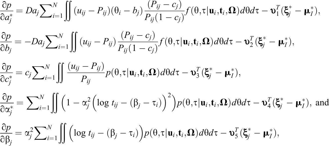
The MML estimator of

where

The above derivatives cannot be calculated yet because of dependence on the unknown quantities resulting from the latent variables (e.g.,
3.2. MMAP Estimation
The MMAP estimator draws inference about the item parameters from a posterior probability distribution. Let

where

The first term in the right-hand side of Equation 8 is the log of the marginal likelihood, which is given in Equation 6. Hence, one only needs to address the additional term corresponding to the prior density.
Assuming the multivariate normal prior for the transformed item parameters in Equation 5, the MMAP estimator of

where
with
4. Optimal Sampling Design
The other critical element to consider in online calibration is sampling design, which prescribes how to collect a calibration sample for an item being field tested. For maximizing information about the parameters of an item, it is ideal to select an optimal sample from a complete pool of test takers. In practice, however, it is difficult to obtain such a static examinee pool because many operational tests are administered continuously or at time intervals. A more viable approach is to select an item from a preconstructed item pool and administer the selected item when an examinee reaches a seeding location for field-testing. This strategy leads to a procedure akin to the operational item selection. That is, as an examinee enters a field-testing stage, all items in the field-testing item pool are evaluated based on their current parameter values and the item that the incumbent examinee can provide with the most optimal properties is selected for administration.
Prior studies have considered three approaches to assign a field-testing item: (1) random selection (e.g., Ban et al., 2001, 2002; P. Chen, 2017; P. Chen & Wang, 2016; P. Chen et al., 2012), (2) examinee-centered selection (e.g., P. Chen et al., 2012, 2017; Zheng, 2016), and (3) item-centered selection (e.g., Chang & Lu, 2010; Ren et al., 2017; van der Linden & Ren, 2014). The random sampling selects an item randomly from a field-testing item pool when an examinee joins the field-testing. The examinee-centered design selects an item following the operational item selection rule, which in most cases, is designed to maximize information about the examinee’s trait level. The third approach, item-centered design, selects an item that the given examinee can provide with the maximum information among the prospective items. Note that, in the random and examinee-centered schemes, the calibration samples can contain little information about the field-tested items as they are not optimized for item calibration. In view of this, the current study employs the item-centered design in the interest of maximum item information and sampling efficiency.
In the joint model of a response and response time, item information retained by an examinee is calculated as

where

Some key features of the item information matrix can be summarized as follows. First, the null submatrices in the off-diagonal blocks indicate that the item parameters from the response and response time models are conditionally independent given the person parameters. That is, the response time model parameters provide no information about the response model parameters once the examinee’s trait parameters have been taken into account. Second, the bottom-right submatrix indicates that information about the response time parameters depends only on
Given the above item information matrix, a number of optimality criteria are applied to choose the most desirable item for a given examinee. The first criterion is D-optimality, which is designed to maximize the determinant of the item information matrix. For estimating the item parameters within the joint modeling framework, the D-optimal sample is obtained as:

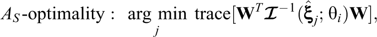
The calibration sample obtained according to the D-optimal criterion will then minimize the volume of a confidence ellipsoid (i.e., generalized variance) of the parameter estimates of the field-tested item. The other criterion considered is A-optimality, which is designed to maximize the trace of the information matrix. In the present context of the joint model, the A-optimal criterion selects an item that minimizes the trace of the inverse of the information matrix:

The calibration sample selected according to the above criterion will minimize average variance of the parameter estimates. For both the optimality criteria, the inverse of the prior covariance matrix (
Observe that the above sampling methods attempt to maximize information about all five item parameters in the joint model. Alternatively, one can optimize the sampling for a subset of the item parameters. For example, if the primary objective of online calibration is to obtain precise estimates of the response model parameters, it would be more desirable to select samples that can provide the most information about the targeted parameters, while using response times as collateral information. In such case, one can adjust the selection criteria to obtain samples that are optimized for the intended parameters. For the D- and A-optimal sampling designs, centering on a subset of parameters leads to

and
respectively, where
Note that, for all the criteria discussed above, the optimality statistics are calculated approximately by replacing the true proficiency parameters with the estimated values. Doing so can induce measurement error when selecting the calibration samples. A practical way of minimizing measurement error is to assign field-testing items at the end of a test, so that the optimality criteria can be evaluated based on the estimates that are sufficiently close to the true proficiency parameter values. The simulation study presented below corroborates that the optimality statistics calculated this way results in only slight loss of sampling efficiency and can still attain nearly optimal samples.
5. Simulation Study
The study performed extensive simulations to evaluate the effectiveness of the proposed online calibration strategies. The simulations were in particular designed to address three questions: (1) overall performance of the suggested online calibration methods, (2) relative performance of joint calibration to regular response model calibration, and (3) an optimal sampling strategy given a particular focus of online calibration.
5.1. Simulation Design
Below presents specific conditions and design variables considered in the simulation study.
Examinee generation: The study assumed a population of 40,000 test takers for administering CAT. The examinees’ trait parameters were randomly sampled from a bivariate normal distribution with zero means and unit variances. The correlation between the proficiency and speed dimensions was set as
Item generation: The operational and field-testing item pools were created with the fixed sizes of 300 and 15, respectively. The parameter values of both the item types were drawn from a multivariate normal distribution with a mean,
Operational CAT administration: The operational CAT was simulated with a total of 30 items. During CAT, items were selected adaptively according to the maximum information criterion. The item selection based on the maximum information rule tends to result in a skewed distribution in item usage. To prevent overexposure of items, the study imposed a constraint on the maximum number of item assignment such that each item can be assigned no more than 800 examinees. The examinee’s trait parameters were estimated via expected a posteriori throughout.
Online calibration: Online calibration of field-testing items was carried out as follows. Each test taker received three field-testing items during operational CAT. The seeding locations of the pilot items were randomly decided in the later stage of testing (i.e., between the 24th and 33rd items) to regulate measurement error. For each prospective item, starting parameter values, which were obtained from a random sample of 300 examinees, were assigned before the outset of online calibration. These parameter values were used to initiate the sampling in the beginning of online calibration. In practice, one can obtain initial parameter values using content experts’ crude approximations or by conducting preparatory online calibration with small samples. As an item sets off the field-testing process, the item was administered to 100 examinees according to the specified sampling strategy. The item parameter values were not updated during this period because the sample was too small to attain stable parameter estimates. Once the item was assigned to the minimum sample of 100 examinees, the parameter values were successively estimated and updated after every batch of 10 additional observations. The adaptive online calibration process continued until the item was assigned to the maximum sample of 800 examinees.
Item parameter estimation: The study employed MMAP as a primary estimation method for calibrating the items. Our preliminary study suggested that the MML estimator tends to have a convergence problem when the calibration samples are selected adaptively. It was surmised that this result is due to little chance of guessing in adaptive sampling. When the lower-asymptote parameters were fixed to a known constant (e.g., the reciprocal of the number of the response options), the MML estimator showed improved convergence rate, but the overall successful convergence rate was still relatively lower than that of the MMAP estimator.
1
Given the findings from the preliminary study, the subsequent simulations were conducted, applying the MMAP as a primary estimator. Note that, although the MML estimator was not used for adaptive online calibration, it can still be of utility in other situations such as linear calibration settings or when prior information is not available.
Sampling design: For every field-testing item, calibration samples were obtained sequentially according to the optimality criterion described in Section 4. The first two criteria select samples that are optimized for all five item parameters; the last two criteria select samples optimized for the response model parameters. To compare the performance of the sampling methods under different scenarios, the study additionally performed online calibration of the response model. The sampling methods evaluated within each calibration model are: random, D-optimal, and A-optimal sampling for the response model calibration; and random, D- and
Replication: The design factors were carefully crossed to contrast the performance of the different online calibration scenarios. In total, 24 simulation conditions were examined—two calibration models, different sampling designs (random, D-,
5.2. Evaluation
The study considered a number of criteria to evaluate the performance of the online calibration procedures. First, relative efficiency statistic (Berger, 1991, 1994) was employed to examine the impact of measurement error on sampling efficiency:
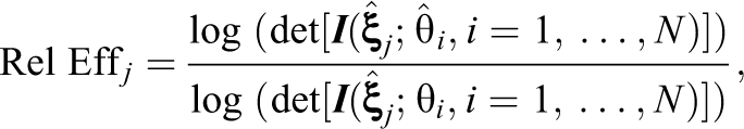
where
The precision of the estimated parameter values was evaluated via bias, root mean squared error (RMSE), correlation, and standard error. The bias and RMSE were calculated respectively as

where J is the number of the field-tested items,
For every evaluation criterion, the study summarizes the results within the specified online calibration scenario. Because each online calibration strategy produced a unique set of field-testing items calibrated, the summary statistics are not necessary based on the same set of field-tested items. As such, the results below should be considered as outcomes that would have been observed under each online calibration scenario when the same item pools were submitted for online calibration—rather than the outcomes based on the same set of field-tested items.
6. Results
6.1. Computation
The computational efficiency of the suggested online calibration methods is briefly reported here. On the whole, the procedures demonstrated high computational efficiency throughout the simulation. On a desktop computer with 3.4 GHz processor and 8GB of memory, calibrating an item under the joint model took .851 seconds on average until it reached to the maximum sample size. Calibration under the response model took .017 seconds under the same conditions. The difference in computing times across the different sampling methods was minimal because of the small number of field-testing items considered.
6.2. Relative Efficiency
Figure 1 presents boxplots of the relative efficiency statistics observed for each sampling design. The plots suggest that the sampling procedures generally maintained high efficiency in selecting the calibration samples despite the measurement error. The relative efficiency statistics were close to one and remained constant across the different calibration scenarios. Although the sampling methods seemed to slightly lose efficiency due to measurement error, the overall magnitude of the loss was in general insignificant. Figure 1 also reveals a consistent pattern with regard to the calibration models. The joint model steadily demonstrated higher sampling efficiency and showed smaller variation compared to the response model. This tendency seems to indicate that the use of response times in online calibration can alleviate the loss of sampling efficiency caused by measurement error and leads to more efficient and stable sampling. In particular, the improvement in the sampling efficiency further escalated when the joint model was calibrated based on the optimal samples. Among the different sampling methods considered, the A-optimal procedures generally showed the highest sampling efficiency, followed by the D-optimal and random sampling methods.

Relative efficiency of sampling designs.
6.3. Bias
Table 1 presents biases of the response model parameter estimates observed at the fixed calibration points,
Bias of the Item Parameter Estimates for the Response Model
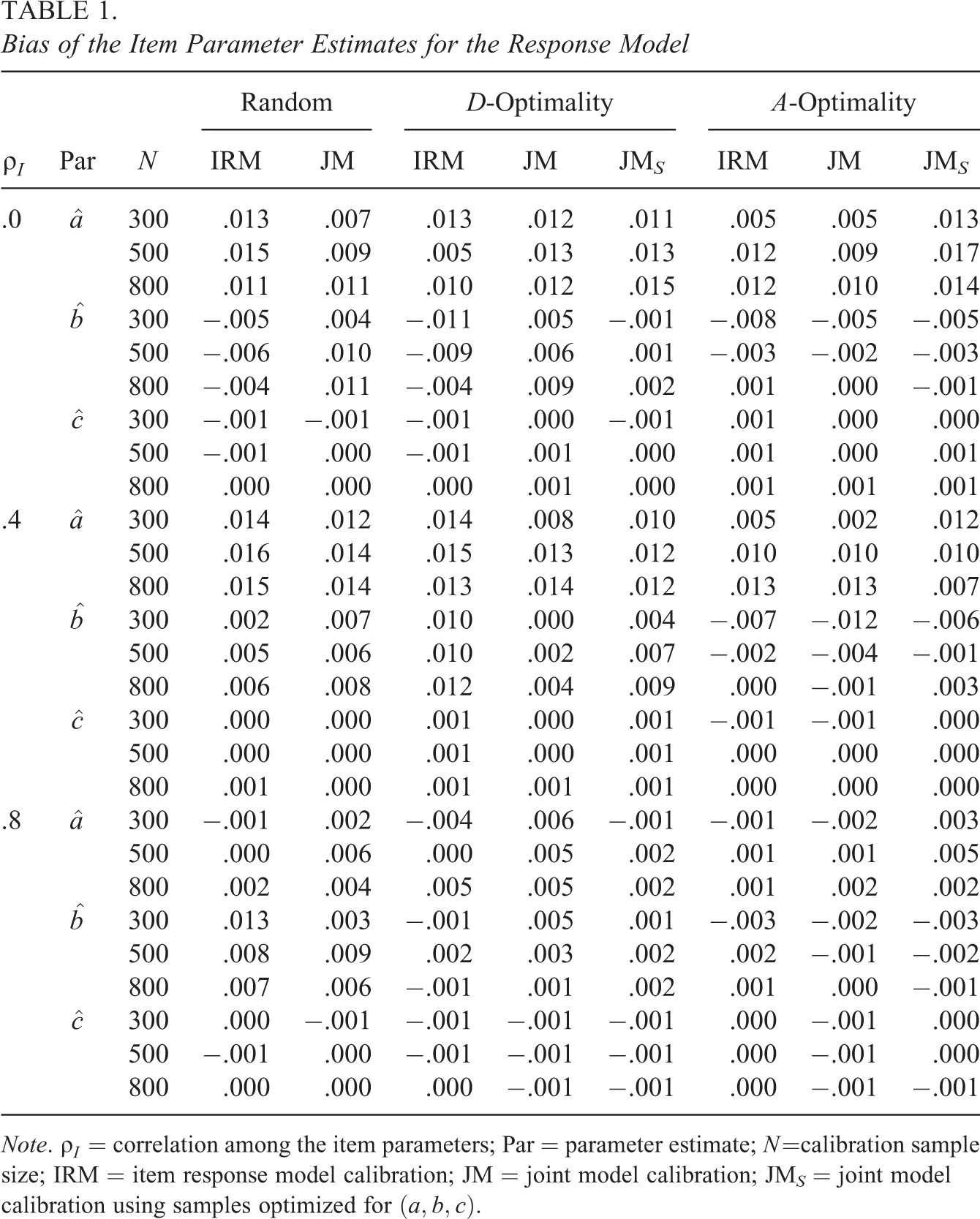
Note.
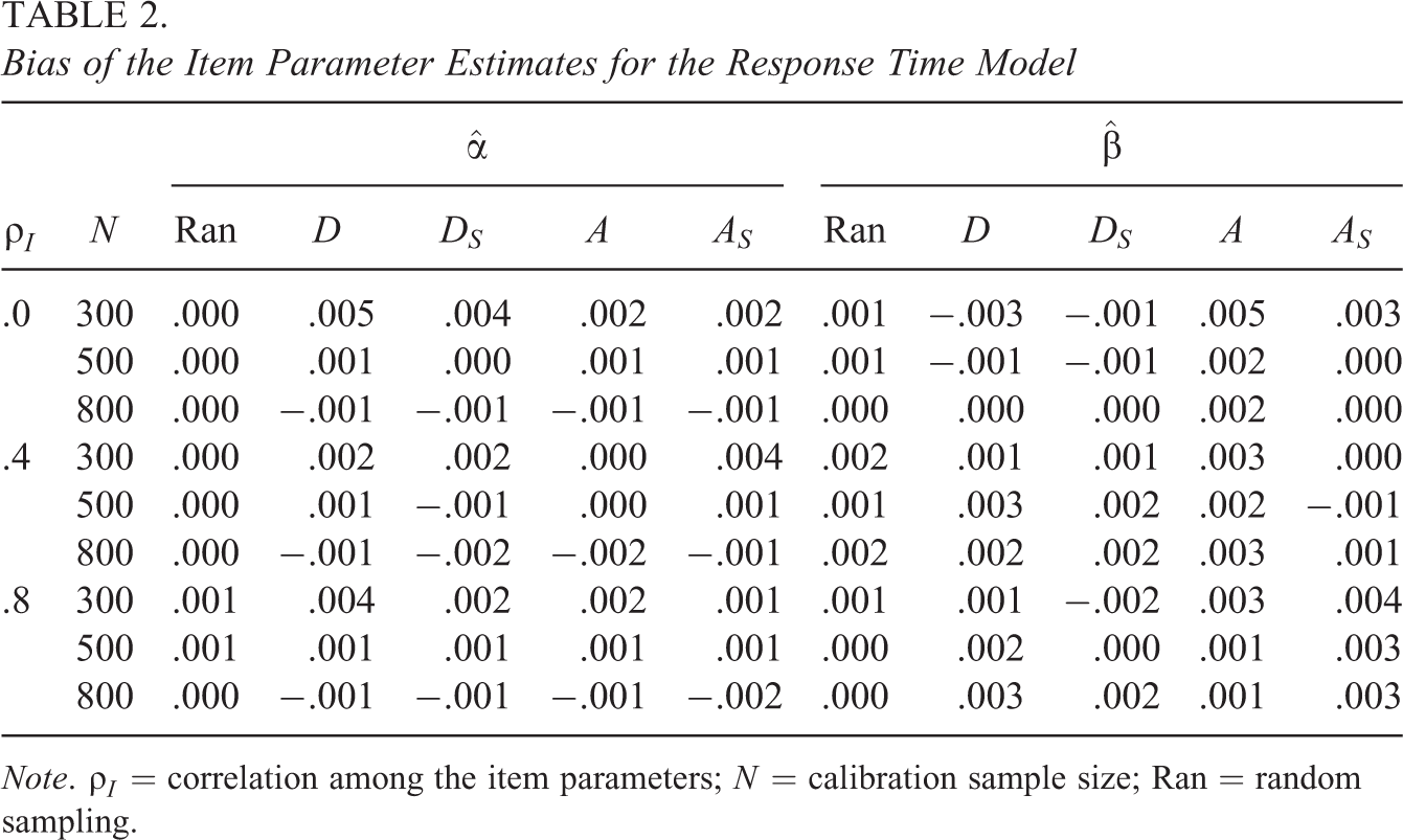
Table 2 presents biases of the response time model parameter estimates. The observed statistics were again very close to zero, implying that the parameter estimates were essentially unbiased. The largest bias observed was .005, and the values appropriately decreased as N increased. Among the sampling methods, random sampling led to the smallest bias though the difference with the other designs appeared minimal.
Bias of the Item Parameter Estimates for the Response Time Model
Note.
6.4. RMSE
Tables 3 and 4 provide average RMSEs of the item parameter estimates for the response and response time models, respectively. As with the previous, the results are summarized for the fixed calibration points. More detailed reports are presented as figures in Appendix C in the online version of the journal. The tables suggest that the online calibration performed reasonably well in recovering the true item parameter values. The RMSEs were constantly small across the varying simulation conditions and decreased appropriately as the calibration progressed. In particular, the item parameter estimates showed fast convergence to the generating parameters in the very early stage of online calibration. For example, when
One of the inquiries made in this study was the relative performance of joint calibration to standard response model calibration. A comparison of the two models in Table 3 suggests that they tend to perform comparably when the item parameters are uncorrelated. When the parameters were correlated, joint calibration showed distinct improvement in estimation of the response model parameters. In particular, when
RMSEs of the Item Parameter Estimates for the Response Model

Note.
The other research question posed in this study was the performance of sampling design given a specific focus of online calibration. For evaluation, the study considered two situations: when the primary interest of online calibration is (1) in estimating all five item parameters accurately and (2) in estimating the response model parameters only. For the former, three sampling methods (random, D-, and A-optimality) were evaluated within the joint model. For the latter, all eight sampling methods were evaluated under both the response and joint models to gauge the benefit of utilizing response times in online calibration. In each scenario, multiple factors (e.g., item parameter type,
The results from Tables 3 and 4 suggest that, when all the item parameters are intended for estimation and the item parameters are weakly or moderately correlated, joint calibration with A-optimal sampling would lead to the most stable parameter recovery. A-optimality was especially found effective in minimizing the RMSE of
RMSEs of the Item Parameter Estimates for the Response Time Model

Note.
To decide an optimal sampling scheme in the second scenario, careful deliberation was again exercised. The results from Table 3 suggest that when online calibration was aimed at the response model parameters and the parameters had zero correlation, joint calibration with
Notice that the above evaluation steadily preferred the joint calibration over the response model calibration despite the fact that the online calibration was aimed at the response model parameters. The gain in the estimation precision accomplished by the joint calibration was especially greater when the items were calibrated using the optimal samples or when the item parameters were correlated to a stronger degree. When the item parameters were weakly related, centering the sampling design on the targeted parameter set seemed to minimize the calibration error for the intended item parameters. When the item parameters had strong correlation, it was more advantageous to optimize the sampling for all the item parameters rather than aiming for the subset of the parameters.
6.5. Correlation
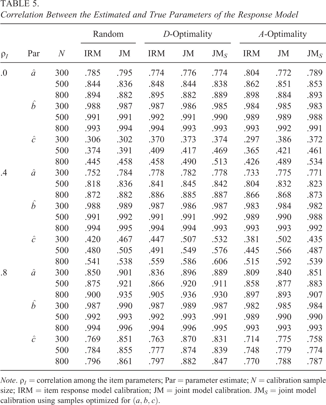
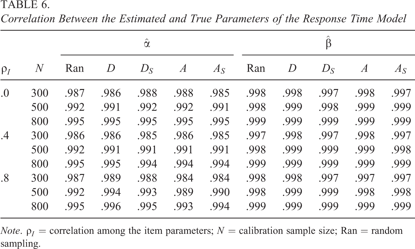
Tables 5 and 6 present average correlations between the estimated and generated item parameters for the response and response time models, respectively. We note that, although the results were summarized using the average of the statistics, the correlations tended to display left-tailed distributions. 3 We thus advise prudence in interpreting the results as they may not represent typical outcomes due to the presence of extreme values. For more detailed representation of the results, see the online Appendix C.
Correlation Between the Estimated and True Parameters of the Response Model
Note.
Correlation Between the Estimated and True Parameters of the Response Time Model
Note.
The tables suggest that the estimated item parameter values overall had stable linear relationships with the generating parameters. The correlations remained reasonably large across the different situations and increased appropriately as N or
The preference for the sampilng method varied depending on the objective of online calibration and correlation among the item parameters. The results from the tables suggest that, when all the item parameters are intended for estimation and the parameters are uncorrelated, joint calibration with A-optimal sampling would lead to the most stable performance. When the item parameters had nonzero correlation, calibrating items jointly based on the D-optimal samples was most preferred. It is pertinent to note that, in the above evaluations, the random sampling tended to yield the highest correlations in
When the focus of online calibration was on the response model parameters and the parameters were uncorrelated, joint calibration based on optimal samples showed little advantage in improving the correlation between the true and estimated parameter values. When the item parameters were correlated to some extent, however, joint calibration tended to yield higher correlation outcomes. When
6.6. Standard Error
Tables 7 and 8 report standard errors of the estimated item parameters for the response and response time models, respectively. Again, it is to be noted that, although the results were summarized using the average of the statistics, the observed standard errors tended to show right-tailed distributions. 4 We therefore advise to exercise caution when interpreting and comparing the results. See the online Appendix C for more detailed representation of the results. The results from the tables suggest that online calibration performed reasonably well, resulting in small standard errors. The two modeling schemes showed no systematic differences in the standard errors. On the whole, the most influential factor seemed to be the calibration sample size. As N increased, the standard errors became appropriately smaller, indicating more stable estimation of the parameters.
Standard Errors of the Item Parameter Estimates for the Response Model

Note. The item parameter estimates were on the transformed scale.
Standard Errors of the Item Parameter Estimates for the Response Time Model

Note.
Table 7 reveals some distinct patterns relating to the sampling design. Among the three sampling methods, the A-optimal procedures steadily produced the smallest standard errors. For example, when
7. Discussion
The nature of speededness in operational tests and free access to response time data in computerized tests have inspired much research on the response times in educational and psychological assessments. In this study, we investigate online calibration strategies for the joint model of responses and response times. The study presented likelihood-based estimators for estimating the parameters of the joint model and evaluated their performance in conjunction with the optimal sampling procedures. Extensive experiments based on simulation suggested that the studied online calibration methods can adequately recover the true item parameters using small samples (N = 500 ∼ 800). Across the evaluated simulation conditions, the estimated parameter values showed small biases and RMSEs, and high correlations with the generating parameters. As expected, increasing N or
One of the questions addressed in this study was whether, if so how much, calibrating items within the joint framework can help improve the estimation of the response model parameters. The results from the current study suggest that joint calibration can lead to more accurate parameter recovery if the item parameters are correlated between the two measurement models. The gain in the estimation accuracy was particularly conspicuous in estimation of c- and a-parameters and tended to escalate as
The other aspect investigated in this study was the performance of the sampling methods given a particular objective of online calibration. A number of sampling procedures were examined to investigate this question: (1) random, D-optimal, and A-optimal sampling under the response model calibration and (2) random, D- and
When the primary focus of online calibration was on a subset of item parameters, centering the sampling design on the targeted parameters within the joint framework was found the most effective approach. The current study in particular contemplated a situation where online calibration was aimed at the response model parameters. The results from the simulation study suggest that when the item parameters are unrelated (i.e.,
It is important to stress that, if the item parameters are strongly correlated, the effect of centering tends to wither, and it is more preferable to use samples that are optimized for all item parameters even though online calibration is aimed at a subset of item parameters. Throughout, we found that when the item parameters are strongly correlated, calibrating items jointly with D-optimal samples tends to produce the most accurate parameter recovery without regard to whether the online calibration is aimed at the entire or subset of the item parameters. This tendency may be partly explained by the fact that D-optimality utilizes information from both the respective and joint relations of the item parameters by maximizing the determinant of the item information matrix. A-optimality, on the other hand, uses information only on the individual item parameters by taking the trace of the inverse information matrix.
As final remarks, we note that the current study assumed known hyperparameters when estimating the item parameters. A future study may extend this setting by considering the hyperparameters as free parameters. It is also worth mentioning that the present study implemented online calibration under the assumption that the pilot items adequately fit the joint model. As indicated by several studies (e.g., Kang, 2017; Klein Entink, van der Linden, & Fox, 2009; Ranger & Kuhn, 2012; Wang, Fan, Chang, & Douglas, 2013), the shape of response time distributions can vary to a large extent across items even within a single test. With this in view, we recommend taking a tryout step prior to online calibration to ensure that probationary items adequately fit the presumed measurement models. This can be achieved in practice by fitting the model with small random samples before the online calibration. Associated with the present concern, it appears promising to study sequential monitoring procedures that evaluate the quality of items over the course of operational assessment. In practice, some items may become compromised when they are used repeated times. The statistical quality control procedure based on online calibration technique can be useful in this event as it can identify items as soon as they become compromised or function differently.
Supplemental Material
Supplemental Material, JEBS879080_Appendix_C - Online Calibration of a Joint Model of Item Responses and Response Times in Computerized Adaptive Testing
Supplemental Material, JEBS879080_Appendix_C for Online Calibration of a Joint Model of Item Responses and Response Times in Computerized Adaptive Testing by Hyeon-Ah Kang, Yi Zheng and Hua-Hua Chang in Journal of Educational and Behavioral Statistics
Footnotes
Appendix A. MML Estimation with EM Algorithm
The EM algorithm adopts an iterative procedure to find maximum likelihood estimates of parameters in the presence of unobserved latent variables. The E-step of the algorithm evaluates expectation of complete-data log-likelihood using provisional estimates of structural parameters. In the context of the joint model, the parameters of an item are considered structural parameters, and individuals’ trait parameters are considered incidental parameters. Suppose we are interested in estimating the parameters of a field-tested item j. For notational simplicity, we suppress the subscript j in the following equations and assume that inference is being made on the parameters of the item j,
where i (
The study evaluates the integrals in (A.1) using the Gauss-Hermite quadrature. Let Xk
(
where
For evaluating (A.1), some expected values are needed to remove dependence on the unobservable variables. In this study, we obtain expected values associated with the incidental parameters as follows:
These quantities are called artificial data because they are created artificially during the estimation. The values of the artificial data still depend on the unknown item parameters (e.g.,
In the M-step, a better approximation to the true parameter is obtained as
where
where
The iterative algorithm continues until changes in the successive approximations become sufficiently small. The present study uses .001 as a stopping criterion for both the EM cycles and Fisher scoring iterations.
Appendix B. MMAP Estimation with EM Algorithm
The EM algorithm in the MMAP estimation is implemented analogously with the MML estimation. Several modifications are however needed to adjust the transformation of the item parameters as well as to incorporate the prior density. Let
where
Let
otherwise,
Declaration of Conflicting Interests
The author(s) declared no potential conflicts of interest with respect to the research, authorship, and/or publication of this article.
Funding
The author(s) disclosed receipt of the following financial support for the research and/or authorship of this article: This study received funding from Campus Research Board (grand ID RB15138).
Notes
References
Supplementary Material
Please find the following supplemental material available below.
For Open Access articles published under a Creative Commons License, all supplemental material carries the same license as the article it is associated with.
For non-Open Access articles published, all supplemental material carries a non-exclusive license, and permission requests for re-use of supplemental material or any part of supplemental material shall be sent directly to the copyright owner as specified in the copyright notice associated with the article.