Optimal Sample Allocation Under Unequal Costs in Cluster-Randomized Trials

Abstract

Conventional optimal design frameworks consider a narrow range of sampling cost structures that thereby constrict their capacity to identify the most powerful and efficient designs. We relax several constraints of previous optimal design frameworks by allowing for variable sampling costs in cluster-randomized trials. The proposed framework introduces additional design considerations and has the potential to identify designs with more statistical power, even when some parameters are constrained due to immutable practical concerns. The results also suggest that the gains in efficiency introduced through the expanded framework are fairly robust to misspecifications of the expanded cost structure and concomitant design parameters (e.g., intraclass correlation coefficient). The proposed framework is implemented in the R package odr.

Keywords

educational reform evaluation experimental design hierarchical linear modeling program evaluation

The statistical power to detect treatment effects in cluster-randomized trials is, in part, governed by how the total sample size is allocated across levels of the hierarchy and treatment conditions (Bloom, 2005; Hedges & Borenstein, 2014; Kelcey et al., 2016; Liu, 2003; Spybrook et al., 2016). For instance, holding constant the total sample size, designs can achieve different levels of statistical power under different sampling plans (Hedges & Borenstein, 2014; Liu, 2003; Raudenbush, 1997). Equally, holding constant the total sample size, designs with different sampling plans may require different total costs because the costs of sampling a unit are not always equal across levels (Hedges & Borenstein, 2014; Raudenbush, 1997) and treatment conditions (Cochran, 1963; Liu, 2003; Nam, 1973).

As a result, an important first step in the design of such studies is to consider theoretical guidelines for sample allocation. Such guidelines have been typically derived from the conventional optimal design framework (e.g., Raudenbush, 1997). The conventional framework seeks to identify the sample allocation that produces the greatest statistical power to detect a treatment effect given a fixed budget by leveraging information regarding the marginal costs of sampling additional clusters and individuals (Hedges & Borenstein, 2014; Liu, 2003; Raudenbush, 1997). Implicit in this framework is the assumption that the costs of sampling additional control and treatment units are invariable.

However, prior theoretical and empirical work in the context of cluster-randomized trials suggests that the marginal costs potentially vary across treatment conditions and sampling levels. The potential for differences in costs of sampling a unit across levels in cluster-randomized trials has been recognized and modeled in previous literature (e.g., Hedges & Borenstein, 2014; Raudenbush, 1997). For example, in a classroom-randomized trial in which classrooms are the primary unit of randomization (e.g., Mosteller, 1995), recruiting one additional classroom is much harder, also more expensive, than sampling one additional student from an already sampled classroom.

The costs of sampling potentially vary between treatment conditions as well (Cochran, 1963; Liu, 2003; Nam, 1973). The marginal cost of sampling a unit in the control condition (C) includes the expenditures used to recruit and measure such a unit (e.g., business travels and work time of data collectors, incentive paid to the unit). The marginal cost of sampling a unit in the treatment condition (C^T) usually includes the same marginal cost of sampling a control unit (C) plus the marginal fees associated with the delivery and implementation of interventions to this unit (C^I; e.g., specialized training to become an intervention provider, work time of an intervention provider), or $C^{T} = C + C^{I}$ . Thus, we have $C^{T} / C = 1 + C^{I} / C$ . That is, the cost ratio of sampling between treatment condition ( $C^{T} / C$ ) is potentially dependent on how expensive interventions are relative to the cost of sampling a control unit ( $C^{I} / C)$ or how cheap sampling a control unit is relative to the marginal cost of interventions.

There are notable examples of studies in which expenses varied across treatment conditions. Take for example the study reported by Springer et al. (2011) regarding a cluster-randomized evaluation of whether incentives in teacher performance improve student outcomes. In this study, teachers in the experimental group were eligible to receive a bonus payment of up to US$15,000 per year based on their students’ performance on tests. In contrast, teachers in the control condition carried on with business as usual. As a result, the costs of sampling each additional teacher in the experimental group typically exceed the cost associated with sampling an additional control teacher.

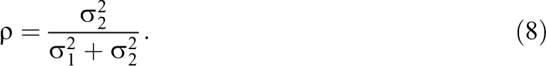
A similar example of differences in costs unfolded in the Tennessee class size experiment (Mosteller, 1995). This experiment evaluated the effects of student–teacher ratios on student achievements (Mosteller, 1995). Students and teachers were randomly assigned to one of three treatment conditions: regular classrooms of 22 to 25 students (the control condition), small classrooms of 13 to 17 students, and regular classrooms of 22 to 25 students assisted by a paid and trained teacher aide. In this setting, classrooms staffed with an aide are likely to incur additional costs as are smaller classrooms.

Examples of differential sampling costs among treatment conditions are not limited to classrooms and schooling. This type of cost disparity often arises in health care. For example, many community health interventions include public education messaging and activities or the general promotion of novel policies (e.g., Glynn et al., 1995) and incorporate costly trainings for health care providers (e.g., Hiscock et al., 2008). In many of these instances, the nature of an intervention and its deployment incurs marginal costs above and beyond those realized in the control condition. A study of 4-year smoking cessation community intervention includes activities of public education, training of health care providers, and promotion of policies to restrict the sale and use of tobacco (Glynn et al., 1995); another intervention is a three-session training program co-led by well child providers and a parenting expert (Hiscock et al., 2008). Some additional examples of costly interventions are 10 days of training and travels to professional development conferences (Greenleaf et al., 2011); 10 two-day on-site training sessions (Jacob et al., 2015); 4-day professional trainings with 1 day per month (Jayanthi et al., 2017).

Although sampling costs plausibly vary across treatment conditions, empirical research suggests that such cost differences are predominantly found at the cluster level where the interventions are implemented (e.g., Liu, 2003; Mosteller, 1995; Springer et al., 2011). The differences in sampling costs at the individual level, if there are any, will be relatively small comparing with the sampling costs at the cluster level.

Even the cost of sampling a unit potentially varies across levels of the design and treatment conditions, the budget functions in previous optimal design frameworks do not fully consider these variations in the cost structures of sampling, and the optimal design parameters chosen to maximize the statistical power in these frameworks are also limited. For example, in the optimal design framework developed by Raudenbush (1997) for two-level cluster-randomized trials, the budget function only considers the cost variation across levels and assumes the cost of sampling one additional individual or cluster in the experimental group is equal to that in the control group. Along with the between-treatment equal cost assumption in the budget function, the Raudenbush (1997) framework optimizes the sampling ratio across levels but not between treatment conditions. Alternatively, Liu (2003) developed a framework that allows cost variation between treatment conditions. Yet, the Liu (2003) framework does not model cost variation across levels and thus optimizes the sampling ratio between treatment conditions but not across levels.

More generally, the perspectives presented in previous frameworks (e.g., Connelly, 2003; Liu, 2003; Raudenbush, 1997; Turner et al., 2004) only partially consider the potential sampling costs of a cluster-randomized trial and optimize the sample ratio either across levels or between treatment conditions. Each of these previous frameworks present a type of constrained optimization—that is, they optimize only one of the sampling ratios across levels and between treatment conditions and constrain the another one. As a result, each of these frameworks potentially returns suboptimal sampling schemes when sampling costs vary across levels of the design and treatment conditions.

In this study, we develop an optimal sampling framework that considers the potential for variation in costs across treatment conditions and levels of the hierarchy. We consider the design of two- and three-level cluster-randomized trials and organize our study as follows. We begin with a review of the literature regarding previous optimal design frameworks. We follow with the development of a more flexible optimal design framework that relaxes the typical parameter and cost constraints for two-level cluster-randomized designs and derives optimal sample allocation across levels and treatment conditions from multiple perspectives. We then extend this framework to three-level cluster-randomized trials. We follow by detailing the relative design precision and efficiency between different sample allocations and subsequently use it to compare the results between the proposed and previous frameworks. In turn, we investigate the robustness of the proposed optimal sample scheme to the misspecification of design parameter values and cost structures. We end with a discussion.

Literature Review

For single-level experiments in which individuals are assigned at random to experimental and control groups, prior literature has developed strategies to maximize statistical power under a fixed budget by minimizing the variance of a treatment effect (Cochran, 1963; Nam, 1973). The historical framework begins with a sample size for the experimental group (n^T) and the control group (n^C) and assumes that the costs of sampling an individual in the experimental and control groups are n^T and n^C. In turn, the total cost or budget function of the study can be described as $m = c^{T} n^{T} + c n$ . Under this conventional framework, sampling is optimized in terms of power when the sampling ratio between treatment conditions under the budget function is

n^{T} / n^{C} = \sqrt{c / c^{T}} .

Once the optimal ratio is identified, the total sample size is a straightforward function of the available budget (through the budget function) or power (through a power formula). Equation 1 shows that the more expensive sampling an individual in the treatment condition is, the smaller the proportion of individuals that should be assigned to the treatment condition. If there is no difference in the cost of sampling between treatment conditions ( $c = c^{T}$ ), the best sampling strategy is to assign an equal number of individuals to each treatment condition. Thus, a balanced design is the best one in terms of statistical power under a fixed budget if, and only if, there is no difference in the costs of sampling an additional individual between treatment conditions.

Compared to single-level experiments that only need to identify the optimal sampling ratio between treatment conditions, cluster-randomized trials need to additionally identify optimal sampling ratio across levels. Literature on the optimal sample size allocation for two-level cluster-randomized trials has separately addressed these two facets of optimal ratio in different frameworks but has not developed expressions to optimize them simultaneously in a single framework.

For example, Raudenbush (1997) developed an optimal design framework for two-level cluster-randomized trials in which there are a total number of J clusters and n individuals in each cluster. The budget function in the framework is $m = J (C_{1} n + C_{2})$ , where C₁ and C₂ are the respective costs of sampling an additional individual and cluster regardless of which treatment condition the unit is assigned to. Given this budget function, the optimal sampling ratio across levels that produces the maximum power under the fixed budget by minimizing the variance of the treatment effect can be identified as

n = \sqrt{\frac{(1 - ρ) (1 - R_{1}^{2})}{ρ (1 - R_{2}^{2})}} \sqrt{\frac{C_{2}}{C_{1}}},

where $ρ$ is the unconditional intraclass correlation coefficient in a population, $R_{1}^{2}$ and $R_{2}^{2}$ are the proportions of outcome variance explained by covariates at the individual and cluster levels, respectively. The cluster-level sample size J is then identified under a budget m or a power formula once the optimal n in Equation 2 is given.

An implicit assumption of the conventional optimal design framework (Raudenbush, 1997) is that the cost of sampling a unit in the treatment condition is equal to that of a unit in the control condition, and only balanced designs with an equal number of clusters in each treatment condition are considered. As a result, the Raudenbush (1997) framework presents a type of constrained optimal design framework in which sample allocations are constrained to designs with an equal sample size and equal sampling costs between treatment conditions. However, such constraints are potentially incongruous with other frameworks that recognize the potential for unequal sampling costs between treatment conditions (Cochran, 1963; Liu, 2003; Nam, 1973) and potentially restrictive in practice (e.g., Greenleaf et al., 2011; Jacob et al., 2015; Mosteller, 1995; Springer et al., 2011) because they limit researchers abilities to identify the sample size allocation that produces the greatest statistical power under a fixed budget.

Liu (2003) relaxed the between-treatment equal cost assumption and the constraint of balanced designs in the Raudenbush (1997) framework and shifted the optimal design in multilevel experiments back to the optimal sample size ratio between treatment conditions in single-level experiments. However, by allowing sampling costs to vary between treatment conditions and considering unbalanced designs, the Liu (2003) framework omitted the optimization of sample size ratio across levels. More specifically, under this framework, a unitary total cost for sampling an additional cluster and its individuals is considered but that total cost is allowed to differ by treatment condition.

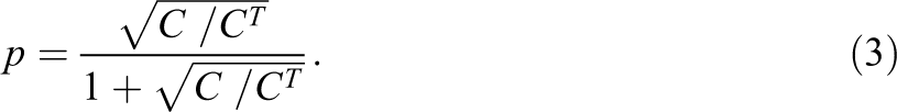
For instance, presume that the combined cost of sampling an additional cluster together with its individuals in the treatment and control groups are C^T and C, respectively. The budget function is $m = (1 - p) J C + p J C^{T}$ with p as the proportion of clusters to be assigned to the treatment condition and J as the number of total clusters.

Under this scenario, Liu (2003) derived the optimal sampling ratio between treatment conditions as $\sqrt{C / C^{T}}$ $(i . e ., (p J) / [(1 - p) J] = \sqrt{C / C^{T}})$ , which has the same expression of Equation 1 for the single-level experiments. Thus, the optimal proportion of clusters to be assigned to the treatment condition is

p = \frac{\sqrt{C / C^{T}}}{1 + \sqrt{C / C^{T}}} .

Although the work by Liu (2003) widened the scope and flexibility of cost structures and is consistent with earlier literature (Cochran, 1963; Nam, 1973), it did not model the cost variation across levels and retained constraints on the sample allocation across levels. Thus, the resulting framework presents a type of constrained optimal design, which often results in suboptimal sample allocation.

The Raudenbush (1997) framework has also been extended to three-level cluster-randomized trials with the same between-treatment equal cost assumption and the balanced-design constraint (Hedges & Borenstein, 2014; Konstantopoulos, 2009, 2011; Moerbeek et al., 2000). Suppose K is the total number of level-three clusters, n and J are the sample sizes per level-two and level-three unit, respectively. The budget function is $m = K (n J C_{1} + J C_{2} + C_{3})$ , where C₁, C₂, and C₃ are the respective costs of sampling one additional level-one, level-two, and level-three unit.

Given the above budget function, the optimal sample allocation across levels in a three-level cluster-randomized trial (Hedges & Borenstein, 2014; Konstantopoulos, 2009, 2011; Moerbeek et al., 2000) as

n = \sqrt{\frac{(1 - ρ_{2} - ρ_{3}) (1 - R_{1}^{2})}{ρ_{2} (1 - R_{2}^{2})}} \sqrt{\frac{C_{2}}{C_{1}}},

and

J = \sqrt{\frac{ρ_{2} (1 - R_{2}^{2})}{ρ_{3} (1 - R_{3}^{2})}} \sqrt{\frac{C_{3}}{C_{2}}},

where $ρ_{2}$ and $ρ_{3}$ are the respective unconditional intraclass correlation coefficient at the level two and level three, and $R_{1}^{2}$ , $R_{2}^{2}$ , $R_{3}^{2}$ are the respective proportions of variance at the level one, level two, and level three explained by covariates. These solutions can be reached in such a way that a three-level cluster-randomized trial is viewed as two-level cluster-randomized trials by omitting level-one or level-three units and then repeating the solution reported under the Raudenbush (1997) framework.

More specifically, by omitting the top-level units, a three-level cluster-randomized trial conceptually reduces to a two-level cluster-randomized trial with an (pseudo) intraclass correlation coefficient of $ρ_{2} / (1 - ρ_{3})$ . By substituting $ρ_{2} / (1 - ρ_{3})$ as the ρ value into Equation 3, we can have the optimal n expression in Equation 4. Likewise, we can have J expression in Equation 5 by omitting the level-one units in a three-level cluster-randomized trial.

Optimal Sample Allocation in Two-Level Cluster-Randomized Trials

We first develop our framework within the context of two-level cluster-randomized trials. We begin with an assumption that sets the individual-level sample sizes to be equal between treatment conditions (i.e., $n = n^{C} = n^{T}$ ). Under the random assignment of clusters, such an assumption simplifies presentation, calculations, and implementation with sacrificing nugatory gains in efficiency. However, we provide the optimal sample allocation solutions without such a constraint in Appendix A.

Models

Assuming a cluster-randomized design, we let the number of sampled individuals in each cluster be n, the number of total sampled clusters be J, and the proportion of clusters to be assigned to the treatment condition be p with $p J$ as an integer. We can estimate the treatment effect through multilevel linear models or ordinary least squares (Raudenbush & Bryk, 2002). Multilevel linear models and ordinary least squares will provide identical treatment effect estimations when the individual-level sample size in the same treatment condition does not vary across clusters. See Hedges and Hedberg (2007) and Hoover (2002) for the method of pooling the variance between treatment conditions when sample sizes are not equal between treatment conditions at the cluster level.

We present the analytic models in the format of multilevel linear models, and the individual-level model is

Y_{i j} = β_{0 j} + β_{I}^{'} X_{i j} + ∊_{i j} ∊_{i j} \sim N (0, σ_{1 |}^{2}),

where $Y_{i j}$ is the continuous outcome of individual i ( $i = 1, 2, \dots, n$ ) in cluster j ( $j = 1, 2, \dots, J$ ), $β_{0 j}$ is the conditional mean score of cluster j, $β_{I} = {(β_{I 1}, \dots, β_{I r})}^{'}$ is an r-length vector of individual-level regression coefficients, $X_{i j}$ is an r-length vector of individual-level covariate values for individual i in cluster j that may vary within and across groups or only within groups, and $∊_{i j}$ is the individual-level error term with a conditional variance $σ_{1 |}^{2}$ .

Similarly, the cluster-level model is

β_{0 j} = γ_{00} + δ T_{j} + γ_{G}^{'} Z_{j} + u_{0 j} u_{0 j} \sim N (0, σ_{2 |}^{2}),

where $γ_{00}$ is the conditional mean across all clusters and individuals, T_j is the treatment indicator with $T_{j} = 1$ for clusters in the treatment group, otherwise $T_{j} = 0$ with $δ$ as the treatment effect. $γ_{G} = {(γ_{G 1}, \dots, γ_{G q})}^{'}$ is a q-length vector of cluster-level regression coefficients, Z_j is a q-length vector of cluster-level covariate values for cluster j, which could include variables measured directly at the cluster level and/or cluster means of individual-level covariates, and $u_{0 j}$ is the random effect of cluster j with a conditional variance $σ_{2 |}^{2}$ . With unconditional variances at the individual and cluster levels as $σ_{1}^{2}$ and $σ_{2}^{2}$ , the intraclass correlation coefficient is

ρ = \frac{σ_{2}^{2}}{σ_{1}^{2} + σ_{2}^{2}} .

If we standardize the outcome to have a variance of one in a population, the treatment effect ( $δ$ ) is placed on a standardized mean difference scale and has a variance of

σ_{δ}^{2} = \frac{ρ (1 - R_{2}^{2}) + (1 - ρ) (1 - R_{1}^{2}) / n}{p (1 - p) J} .

When the null hypothesis is false (i.e., $δ \neq 0$ ), the statistical power follows a noncentral t-distribution (Hedges & Hedberg, 2007; Liu, 2003) with the noncentrality parameter as

λ = \frac{δ}{\sqrt{σ_{δ}^{2}}} = \frac{δ \sqrt{p (1 - p) n J}}{\sqrt{ρ (1 - R_{2}^{2}) n + (1 - ρ) (1 - R_{1}^{2})}} .

The statistical power at the significance level $α$ for the two-tailed test (Donner & Klar, 2000; Hedges & Hedberg, 2007; Hoover, 2002; Rutterford et al., 2015) is

P = 1 - H [c (α / 2, J - q - 2), J - q - 2, λ] + H [- c (α / 2, J - q - 2), J - q - 2, λ],

where $c (α / 2, v)$ is the two-tailed critical value in a t-distribution with v degrees of freedom and the significance level $α$ , and $H (x, v, λ)$ is the cumulative distribution function of the noncentral t-distribution with v degrees of freedom and a noncentrality parameter $λ$ . Similarly, the statistical power at the significance level α for the one-tailed test (Donner & Klar, 2000; Hedges & Hedberg, 2007; Hoover, 2002; Rutterford et al., 2015) is

P = 1 - H [c (α, J - q - 2), J - q - 2, λ] .

Method

The intersection of the optimal design frameworks presented by Raudenbush (1997) and others (Cochran, 1963; Liu, 2003; Nam, 1973), with the cost structures often observed in multilevel studies (e.g., Tennessee class size experiment; Mosteller, 1995), suggests another prospect—the budget function should let the cost of sampling vary across both levels of the hierarchy and treatment conditions. For this reason, we integrate these frameworks to develop a more flexible framework with potentially more realistic cost structures. In this extended framework, we first assign c₁ as the cost of enrolling each additional individual within a cluster in the control condition and $c_{1}^{T}$ as the cost of enrolling each additional individual within a cluster in the treatment condition. Similarly, we use c₂ as the cost of sampling each additional cluster in the control condition and $c_{2}^{T}$ for an experimental cluster.

Thus, the budget function is $m = (1 - p) J (c_{1} n + c_{2}) + p J (c_{1}^{T} n + c_{2}^{T})$ . Rearranging the budget function, we have

J = \frac{m}{(1 - p) (c_{1} n + c_{2}) + p (c_{1}^{T} n + c_{2}^{T})} .

Substituting J in Equation 13 to Equation 9, we can rewrite the variance of the treatment effect as

σ_{δ}^{2} = \frac{[ρ (1 - R_{2}^{2}) n + (1 - ρ) (1 - R_{1}^{2})] [(1 - p) (c_{1} n + c_{2}) + p (c_{1}^{T} n + c_{2}^{T})]}{p (1 - p) n m} .

Optimal Sample Allocation

We can derive optimal sample size allocation from several different but linked perspectives, including minimizing the variance of the treatment effect under a fixed budget, minimizing the budget requested to achieve a fixed variance of the treatment effect, and maximizing the noncentrality parameter $λ$ under a fixed budget. We will have identical results from these different perspectives. Consistent with prior frameworks, we can identify an optimal design that achieves the greatest statistical power under a fixed budget by minimizing the error variance of the treatment effect. To minimize the error variance in Equation 14, we derive its first-order derivatives with respect to p and n and set these derivatives equal to zero, yielding

p = \frac{\sqrt{(c_{1} n + c_{2}) / (c_{1}^{T} n + c_{2}^{T})}}{1 + \sqrt{(c_{1} n + c_{2}) / (c_{1}^{T} n + c_{2}^{T})}},

n = \frac{\sqrt{(1 - ρ) (1 - R_{1}^{2})}}{\sqrt{ρ (1 - R_{2}^{2})}} \sqrt{\frac{(1 - p) c_{2} + p c_{2}^{T}}{(1 - p) c_{1} + p c_{1}^{T}}} .

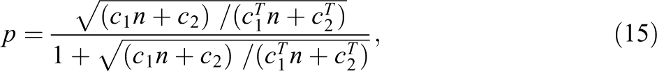
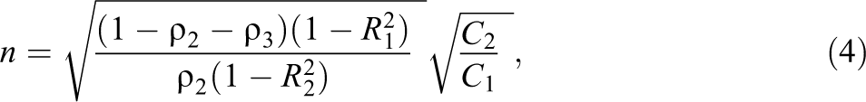
The above expressions can be used to identify the optimal sampling ratio across levels and treatment conditions. There are no simple closed form solutions to the roots of p and n in Equations 15 and 16. We can numerically solve the roots by (1) initiating random values for n (e.g., sample one integer of $n \in (2, 100))$ and calculating an initial value of p using Equation 15; (2) updating the value of n in Equation 16 using the updated p; (3) updating the value of p in Equation 15 using the updated n; (5) Steps 2 and 3 form one iteration. Repeat Steps 2 and 3 until each parameter converges to a specified tolerance level (e.g., $1 / 10^{10}$ ). The resulting converged values of p and n in the final iteration capture the sampling plan that jointly optimizes over these parameters. We implement these solutions in the R package odr (Shen & Kelcey, 2020).

Similar to the results of prior frameworks, the results indicate that the optimal p and optimal n are not a function of total budget m but rather are driven by the relative cost structure of sampling. Only the total number of clusters J is impacted by the total budget through Equation 13. The optimal p is driven by the control/treatment cost ratio of sampling a cluster and its individuals $(i.e., (c_{1} n + c_{2}) / (c_{1}^{T} n + c_{2}^{T}))$ , which is also influenced by the number of individuals sampled in each cluster (n). From Equation 15, we can see that a balanced design with $p = .5$ is the optimal one if, and only if, the costs of sampling a cluster and its individuals in each treatment condition are equal $(i.e., c_{1} n + c_{2} = c_{1}^{T} n + c_{2}^{T})$ . Otherwise, the more expensive sampling a cluster and its individuals in the treatment condition is, the smaller the optimal p. That is, investigators should assign a smaller proportion of clusters to the experimental group when the cost of sampling in the treatment condition is more expensive than that in control.

The optimal n in Equation 16 is driven by two factors. The first factor is the square root of conditional variance ratio between levels $(i.e., \sqrt{σ_{1 |}^{2}} / \sqrt{σ_{2 |}^{2}} = \sqrt{(1 - ρ) (1 - R_{1}^{2})} / \sqrt{ρ (1 - R_{2}^{2})})$ . This indicates that the larger the conditional cluster/individual variance ratio is, the smaller the resulting optimal n. It is intuitive that researchers need more clusters to identify the treatment effect with a larger conditional intraclass correlation coefficient because a larger proportion of variation at the group level requires more clusters to achieve a same level of statistical power or design precision (Hedges & Hedberg, 2007). The terms $(1 - p) c_{2} + p c_{2}^{T}$ and $(1 - p) c_{1} + p c_{1}^{T}$ can be viewed as the weighted costs of sampling one additional cluster and individual, respectively.

The second factor is the square root of the weighted sampling cost ratio between levels, with the proportion of clusters assigned to the experimental group as the weight $(i.e., \sqrt{(1 - p) c_{2} + p c_{2}^{T}} / \sqrt{(1 - p) c_{1} + p c_{1}^{T}})$ . The larger the weighted cluster/individual cost ratio (CICR) is, the bigger the optimal n. Put differently, when the weighted costs of sampling a cluster is more expensive than sampling an individual, researchers should sample fewer clusters in favor of more individuals per cluster.

Constrained Optimal Sample Allocation and Relations to Previous Frameworks

There are practical considerations that may limit the use of optimal sample allocation (Hedges & Borenstein, 2014). For example, many classrooms have an upper limit of about 20 to 30 students, and this may constitute a common constraint in classroom-based designs. We probe several such constraints in p and n in order to (a) delineate the conditions under which the proposed framework reduces to previous frameworks and (b) outline the flexibility of the proposed framework.

Constrained p

Suppose the constrained proportion of clusters to be assigned to the treatment condition is p₀ (i.e., $p = p_{0}$ ). If we minimize the variance of the treatment effect in Equation 14 with respect to n, the constrained optimal individual-level sample size has the exact same expression with Equation 16. Thus, the constrained optimal individual-level sample size can be obtained from Equation 16 along with $p = p_{0}$ . If we let $p = .5$ , $C_{1} = (1 - p) c_{1} + p c_{1}^{T}$ , and $C_{2} = (1 - p) c_{2} + p c_{2}^{T}$ , the constrained optimal individual-level sample size in Equation 16 will reduce to Equation 2, the optimal sample size expression under the Raudenbush (1997) framework.

Constrained n

Suppose the constrained individual-level sample size is n₀ (i.e., $n = n_{0}$ ), minimizing the variance of the treatment effect in Equation 14 with respect to p the constrained optimal proportion has the exact same expression with Equation 15. Thus, the constrained optimal proportion can be obtained from Equation 15 along with $n = n_{0}$ . If we let $C = c_{1} n_{0} + c_{2}$ and $C^{T} = c_{1}^{T} n_{0} + c_{2}^{T}$ , the constrained optimal proportion in Equation 15 will reduce to Equation 3, the optimal p expression under the Liu (2003) framework.

Optimal Sample Allocation in Three-Level Cluster-Randomized Trials

Similar to those for two-level cluster-randomized trials, the potential gains in design efficiency and/or statistical power in three-level cluster-randomized trials can mostly be achieved by optimizing sampling ratios between treatment conditions and among levels. We subsequently present the optimal sample allocation with the constraint of equal sample sizes at the individual and subcluster levels (i.e., $n = n^{C} = n^{T}$ and $J = J^{C} = J^{T}$ ). We provide the optimal sample allocation solutions without such a constraint in Appendix B.

Models

Suppose a three-level cluster sampling design has a total number of K clusters (level-three units) with $p K$ clusters assigned to the treatment condition; each cluster has J subclusters (level-two units) of size n. Let $Y_{i j k}$ be the continuous outcome of unit i in subcluster j in cluster k with $i = 1, \dots, n$ , $j = 1, \dots, J$ , and $k = 1, \dots, K$ . Let $X_{i j k}$ , $Z_{j k}$ , W _k be the vectors of covariates at the level one, level two, level three with corresponding regression coefficient vectors of $β_{I}$ , $β_{J}$ , $β_{K}$ and lengths of r, s, q, respectively. Similar to models for two-level cluster-randomized trials, the covariates could be variables measured at the same level or aggregated values of variables measured at a lower level.

When the sample size per (sub-)cluster does not vary across (sub-)clusters within each treatment condition, we can estimate the treatment effect using ordinary least squares or multilevel linear models (Raudenbush & Bryk, 2002). Under the multilevel formulation, the level-one model is

Y_{i j k} = β_{0 j k} + β_{I}^{'} X_{i j k} + ∊_{i j k} ∊_{i j k} \sim N (0, σ_{1 |}^{2}),

where $β_{0 j k}$ is the conditional mean score of subcluster j in cluster k, and $∊_{i j k}$ is the individual-level error term with a conditional variance $σ_{1 |}^{2}$ . Similarly, the level-two or sub-cluster-level model is

β_{0 j k} = γ_{00 k} + β_{J}^{'} Z_{j k} + u_{0 j k} u_{0 j k} \sim N (0, σ_{2 |}^{2}),

where $γ_{00 k}$ is the conditional mean score of cluster k, and $u_{0 j k}$ is the random effect of subcluster j in cluster k with a conditional variance $σ_{2 |}^{2}$ . The level-three or cluster-level model is

γ_{00 k} = π_{000} + δ T_{k} + β_{K}^{'} W_{k} + u_{00 k} u_{00 k} \sim N (0, σ_{3 |}^{2}),

where $π_{000}$ is the conditional mean across all clusters, subclusters, and individuals, T_k is the treatment indicator with $T_{k} = 1$ for clusters in the experimental group and otherwise $T_{k} = 0$ with $δ$ as the treatment effect, $u_{00 k}$ is the random effect of cluster k with a conditional variance $σ_{3 |}^{2}$ .

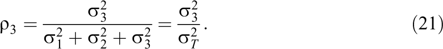
Let the unconditional variances at the individual-, sub-cluster-, and cluster-level be $σ_{1}^{2}$ , $σ_{2}^{2}$ , and $σ_{3}^{2}$ , respectively. The total unadjusted variance is $σ_{T}^{2} = σ_{1}^{2} + σ_{2}^{2} + σ_{3}^{2}$ . The intraclass correlation coefficient at the level two is

ρ_{2} = \frac{σ_{2}^{2}}{σ_{1}^{2} + σ_{2}^{2} + σ_{3}^{2}} = \frac{σ_{2}^{2}}{σ_{T}^{2}} .

The intraclass correlation coefficient at the level three is

ρ_{3} = \frac{σ_{3}^{2}}{σ_{1}^{2} + σ_{2}^{2} + σ_{3}^{2}} = \frac{σ_{3}^{2}}{σ_{T}^{2}} .

If we standardize the outcome to have a variance of one, the treatment effect ( $δ$ ) is placed on a standardized mean difference scale and has a variance of

σ_{δ}^{2} = \frac{n J ρ_{3} (1 - R_{3}^{2}) + n ρ_{2} (1 - R_{2}^{2}) + (1 - ρ_{2} - ρ_{3}) (1 - R_{1}^{2})}{p (1 - p) n J K},

where $R_{3}^{2}$ , $R_{2}^{2}$ , and $R_{1}^{2}$ are the proportions of outcome variance explained by covariates at the cluster, subcluster, and individual levels, respectively.

When the null hypothesis is false (i.e., $δ \neq 0$ ), the statistical power follows a noncentral t distribution with the noncentrality parameter as

λ = \frac{δ}{\sqrt{σ_{δ}^{2}}} = \frac{δ \sqrt{p (1 - p) n J K}}{\sqrt{n J ρ_{3} (1 - R_{3}^{2}) + n ρ_{2} (1 - R_{2}^{2}) + (1 - ρ_{2} - ρ_{3}) (1 - R_{1}^{2})}} .

Statistical power for three-level cluster-randomized trials can be obtained by inserting the above noncentrality parameter into Equation 11 for the two-tailed test or Equation 12 for the one-tailed test with substituting J as K in the degree of freedom expression.

Optimal Sample Allocation

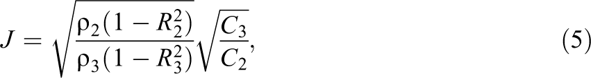
Suppose the respective costs of enrolling each additional level-one, level-two, and level-three unit in the control condition are c₁, c₂, and c₃, and the costs of enrolling each additional level-one, level-two, and level-three unit in the treatment condition are $c_{1}^{T}$ , $c_{2}^{T}$ , and $c_{3}^{T}$ , respectively. Thus, the budget function is $m = (1 - p) K (c_{1} n J + c_{2} J + c_{3}) + p K (c_{1}^{T} n J + c_{2}^{T} J + c_{3}^{T})$ . Rearranging the budget function, we have

K = \frac{m}{(1 - p) (c_{1} n J + c_{2} J + c_{3}) + p (c_{1}^{T} n J + c_{2}^{T} J + c_{3}^{T})} .

Substituting K in Equation 24 to Equation 22, we have the variance of the treatment effect as

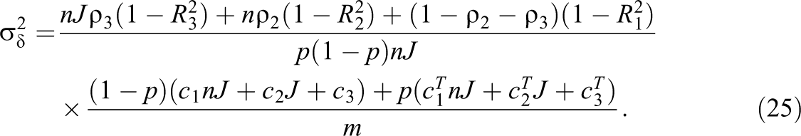
σ_{δ}^{2} = \frac{n J ρ_{3} (1 - R_{3}^{2}) + n ρ_{2} (1 - R_{2}^{2}) + (1 - ρ_{2} - ρ_{3}) (1 - R_{1}^{2})}{p (1 - p) n J} \frac{(1 - p) (c_{1} n J + c_{2} J + c_{3}) + p (c_{1}^{T} n J + c_{2}^{T} J + c_{3}^{T})}{m} .

Following similar methods of minimizing the error variance of the treatment effect, the optimal sampling plan for each parameter can then be delineated as

p = \frac{\sqrt{(c_{3} + c_{2} J + c_{1} n J) / (c_{3}^{T} + c_{2}^{T} J + c_{1}^{T} n J)}}{1 + \sqrt{(c_{3} + c_{2} J + c_{1} n J) / (c_{3}^{T} + c_{2}^{T} J + c_{1}^{T} n J)}},

n = \sqrt{\frac{(1 - ρ_{2} - ρ_{3}) (1 - R_{1}^{2})}{ρ_{3} (1 - R_{3}^{2}) J + ρ_{2} (1 - R_{2}^{2})}} \sqrt{\frac{(1 - p) (c_{3} + c_{2} J) + p (c_{3}^{T} + c_{2}^{T} J)}{(1 - p) c_{1} J + p c_{1}^{T} J}},

J = \sqrt{\frac{n ρ_{2} (1 - R_{2}^{2}) + (1 - ρ_{2} - ρ_{3}) (1 - R_{1}^{2})}{n ρ_{3} (1 - R_{3}^{2})}} \sqrt{\frac{(1 - p) c_{3} + p c_{3}^{T}}{(1 - p) (c_{2} + c_{1} n) + p (c_{2}^{T} + c_{1}^{T} n)}} .

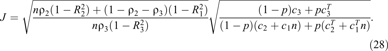
Each of the expressions in Equations 26 through 28 identifies the optimal sampling plan when one of the parameters is malleable. When all three of these parameters are freed, there are no simple closed-form solutions. However, we can solve the multivariate partial derivatives numerically. We implement these solutions in the R package odr (Shen & Kelcey, 2020).

Implications

The optimal design parameters in Equations 26 through 28 provide a more flexible framework for identifying optimal sample allocations across levels and treatment conditions. These optimal design parameters are driven by cost structure and design parameters in a similar but extended fashion with those in two-level cluster-randomized trials. These equations can also be used to improve the precision of cluster-randomized trials with additional constraints. For any given constraint, one just needs to use the relevant constraint to substitute the corresponding optimal design parameter expressions and solve the remaining equations. For example, researchers may constrain the level-one sample size per level-two unit as 20 (i.e., $n = 20$ ), the constrained optimal sample allocation would be solved by using $n = 20$ to substitute Equation 27 and solving the roots of p and J from Equations 26 and 28.

Again, we can see that a balanced design with $p = .5$ is the optimal one if and only if the costs of sampling a cluster and its subsequent subunits in each treatment condition are equal (i.e., $c_{3} + c_{2} J + c_{1} n J = c_{3}^{T} + c_{2}^{T} J + c_{1}^{T} n J$ ). When we additionally let $p = .5$ , $C_{1} = (1 - p) c_{1} + p c_{1}^{T}$ , $C_{2} = (1 - p) c_{2} + p c_{2}^{T}$ , and $C_{3} = (1 - p) c_{3} + p c_{3}^{T}$ , the above optimal sample allocation expressed in Equations 27 and 28 reduces to solutions in previous frameworks but with different formulations (Hedges & Borenstein, 2014; Konstantopoulos, 2009, 2011).

Relative Precision (RP) and Relative Cost Efficiency (RCE)

There are many practical reasons that may constrain the use of the optimal sampling allocation guidelines derived above. From a practical standpoint, for instance, the number of clusters available to researchers in a particular study may be below the number suggested by the formulas. In response, researchers may intentionally expend resources by sampling additional individuals within clusters in an attempt to compensate for this constraint. Similarly, from a design standpoint, we may eventually find that the parameter values used to plan a study differ from the observed values. Here, we suffer from a type of design misspecification because the proposed optimal sampling plan (based on predicted values) may prove to be suboptimal once data have been collected. When the optimal sample allocation is not a viable option or was incorrectly identified, we can identify the specific loss of statistical precision and efficiency an alternative design presents relative to the true optimal design (based on true values). Such statistical precision and efficiency analyses help provide a sense of what constitutes efficient designs and can assist researchers in identifying designs with the most statistical precision and efficiency among the many constrained designs that may be viable.

Our analysis of statistical precision and design efficiency considers two complementary planning perspectives. In the first perspective, we consider the statistical precision as measured through the relative variance of studies in which the sampling plan is malleable, but the budget and remaining parameters are constrained to preset values. In this setting, we compare the variances of the treatment effect estimator under a suboptimal sampling plan with that of an optimal sampling plan. Conceptually, this assessment of relative statistical precision captures the increased sampling variance incurred by using suboptimal sample allocations. To facilitate interpretations using a common metric, we subsequently frame this analysis in terms of the minimum detectable effect size (MDES; Bloom, 1995) because the MDES is a design parameter that researchers often use in planning studies.

In the second perspective, we consider the relative efficiency of designs in terms of study cost such that the total budget is now free, but the effect size, statistical power, and other parameters are fixed. Under this approach, we detail the total additional cost a study under suboptimal sampling would require to achieve an error variance comparable to a study that used optimal sampling. Conceptually, this evaluation quantifies the increased resources required to carry out suboptimal designs.

For the first perspective, the RP is

RP = \frac{σ_{δ^{o}}^{2}}{σ_{δ}^{2}},

where $σ_{δ^{o}}^{2}$ is the smallest possible variance of the treatment effect a type of trial can achieve under a fixed budget, and $σ_{δ}^{2}$ is the variance of the treatment effect an alternative and suboptimal design can achieve under the same budget.

For the second perspective, we can define RCE as

RCE = \frac{m^{o}}{m},

where m^o is the smallest budget to achieve a desired level of variance of the treatment effect (or statistical power) under the optimal sample allocation, and m is the budget to achieve the same level of design precision under an alternative and suboptimal design.

Using information from Equation 14, both perspectives share a more general relative precision and efficiency (RPE) expression for a suboptimal design relative to the optimal design for two-level cluster-randomized trails as

RPE = \frac{[ρ (1 - R_{2}^{2}) n^{o} + (1 - ρ) (1 - R_{1}^{2})] [(1 - p^{o}) (c_{1} n^{o} + c_{2}) + p^{o} (c_{1}^{T} n^{o} + c_{2}^{T})] p (1 - p) n}{[ρ (1 - R_{2}^{2}) n + (1 - ρ) (1 - R_{1}^{2})] [(1 - p) (c_{1} n + c_{2}) + p (c_{1}^{T} n + c_{2}^{T})] p^{o} (1 - p^{o}) n^{o}},

where p^o and n^o represent the optimal design parameter values or the roots of p and n in Equations 15 and 16, and n and p represent the alternative parameter values identified under a different framework or a study actually carried out. The values of RPE range from 0 to 1, with the RPE approaching 1 when a suboptimal design achieves a precision level near the optimal design benchmark. Comparing with the optimal design benchmark, the percentage of increased variance/budget by a study is $(1 - RPE) / RPE \times 100 %$ . RPE values of at least .90 are generally considered good, and an RPE between .80 and .90 is considered acceptable (Hedges & Borenstein, 2014; Korendijk et al., 2010).

Unlike power, effect size, or sample sizes, the variance of the treatment effect is not the simplest design parameter researchers usually face. To systematically improve statistical precision for designs, it is important to transfer such a measure to the ultimate parameter researchers can directly consider. We can further transfer the measure under the first perspective. Let the statistical power and the budget be fixed between the optimal and suboptimal designs and further compare the relative values of MDES between two designs. Under this perspective, the statistical power and thus the noncentrality parameter $λ$ are equal between optimal and suboptimal designs.

Thus, we have $λ = λ^{o}$ or $δ / \sqrt{σ_{δ}^{2}} = δ^{o} / \sqrt{σ_{δ^{o}}^{2}}$ with the additional subscripts to denote parameters in the optimal design. Rearranging this equation, we have

δ^{o} = δ \sqrt{RPE},

where $δ^{o}$ and $δ$ are the respective MDES in the optimal and suboptimal designs under a same budget to maintain the same level of statistical power. Equation 32 quantifies the relative statistical precision, measured by MDES, between an optimal and suboptimal design; thus, it can be used to improve statistical precision by carefully choosing the best available optimal sample allocation and MDES. A design with an RPE of .90 can detect about a 5% smaller effect if it uses the optimal design ( $\sqrt{0.90} \approx 0.95$ ). A design with an RPE of .80 can detect about a 11% smaller effect if the optimal design is used ( $\sqrt{0.80} \approx 0.89$ ). Additionally, given specific design parameters, researchers can directly compute the relative statistical power of a suboptimal and optimal design by using statistical power formulas (Equation 11 or 12).

Similarly, the RPE for a suboptimal design relative to the optimal design for three-level cluster-randomized trails is

RPE = \frac{n^{o} J^{o} ρ_{3} (1 - R_{3}^{2}) + n^{o} ρ_{2} (1 - R_{2}^{2}) + (1 - ρ_{2} - ρ_{3}) (1 - R_{1}^{2})}{n J ρ_{3} (1 - R_{3}^{2}) + n ρ_{2} (1 - R_{2}^{2}) + (1 - ρ_{2} - ρ_{3}) (1 - R_{1}^{2})},

\frac{[(1 - p^{o}) (c_{1} n^{o} J^{o} + c_{2} J^{o} + c_{3}) + p^{o} (c_{1}^{T} n^{o} J^{o} + c_{2}^{T} J^{o} + c_{3}^{T})] p (1 - p) n J}{[(1 - p) (c_{1} n J + c_{2} J + c_{3}) + p (c_{1}^{T} n J + c_{2}^{T} J + c_{3}^{T})] p^{o} (1 - p^{o}) n^{o} J^{o}},

where p^o, n^o, and J^o represent the solved values for optimal design parameters expressed in Equations 26 –28, respectively. p, n, and J represent the actual values a three-level design carried out or identified under a different framework.

A Comparison With Previous Frameworks

In the derivation section, we have shown that previous optimal design frameworks for two-level cluster-randomized trials (Liu, 2003; Raudenbush, 1997) are special cases of our proposed framework. The optimal design parameters for two-level cluster-randomized trials are n and p in our proposed framework. They are n and the constraint of $p = .5$ in the Raudenbush (1997) framework, p and a predetermined value of n in the Liu (2003) $framework$ . Both previous frameworks can be viewed as constrained optimal designs in our proposed framework. Thus, we can directly assess the RPE values of designs identified by previous frameworks comparing with the benchmark designs identified under our proposed framework. Since the conclusion for three-level cluster-randomized trials is the same for two-level cluster-randomized trials, next we only present the results for two-level cluster-randomized trials.

For the cost structures, we considered both equal and unequal costs between treatment conditions and set the cost of sampling one additional individual in the control condition as one (i.e., $c_{1} = 1$ ). For the equal costs between treatment conditions, we considered CICRs as 3, 10, and 30 to reflect potential differences in the costs of sampling a cluster and an individual within a cluster (e.g., Raudenbush, 1997) and presented them in the first three rows of the left panel in Table 1. We considered two scenarios for the unequal costs between treatment conditions. The first scenario fixes the CICR in the control condition as 10 and considers a cluster-level treatment to control cost ratio of 3 (e.g., efficacy studies of interventions; Greenleaf et al., 2011; Jacob et al., 2015), 10 (e.g., teacher pay for performance; Springer et al., 2011), and 30 (e.g., Tennessee class size experiment; Mosteller, 1995). These cost structures are presented in rows 4 through 6 of the left panel in Table 1. The second scenario considers the CICR in the control condition as 3 or 10 and varies the treatment/control cost ratio (TCCR) as those of first scenario (3, 10, 30) but at both the cluster and individual levels. These cost structures are presented in rows 7 through 12 of the left panel in Table 1.

Table 1.

Comparison of Proposed Framework With Previous Frameworks for Two-Level Cluster-Randomized Trials

Cost Structures	$ρ$	Proposed			Raudenbush				Liu
Cost Structures	$ρ$	p	n	J	n	J	RPE	Pr	p	J	RPE	Pr
$c_{1}^{T} = 1$ , $c_{2} = c_{2}^{T} = 3$	.15	.50	6	172	6	172	1.0	.80	.50	94	.72	.65
$c_{1}^{T} = 1$ , $c_{2} = c_{2}^{T} = 3$	.25	.50	4	247	4	247	1.0	.80	.50	130	.59	.56
$c_{1}^{T} = 1$ , $c_{2} = c_{2}^{T} = 10$	.15	.50	11	121	11	121	1.0	.80	.50	94	.91	.76
$c_{1}^{T} = 1$ , $c_{2} = c_{2}^{T} = 10$	.25	.50	8	174	8	174	1.0	.80	.50	130	.81	.71
$c_{1}^{T} = 1$ , $c_{2} = c_{2}^{T} = 30$	.15	.50	18	98	18	98	1.0	.80	.50	94	1.0	.80
$c_{1}^{T} = 1$ , $c_{2} = c_{2}^{T} = 30$	.25	.50	13	145	13	145	1.0	.80	.50	130	.97	.79
$c_{1}^{T} = 1$ , $c_{2} = 10$ , $c_{2}^{T} = 30$	.15	.43	14	111	15	105	.98	.79	.44	96	.98	.79
$c_{1}^{T} = 1$ , $c_{2} = 10$ , $c_{2}^{T} = 30$	.25	.42	10	163	11	154	.97	.79	.44	131	.91	.76
$c_{1}^{T} = 1$ , $c_{2} = 10$ , $c_{2}^{T} = 100$	.15	.34	21	103	25	88	.91	.76	.33	106	1.0	.80
$c_{1}^{T} = 1$ , $c_{2} = 10$ , $c_{2}^{T} = 100$	.25	.32	15	160	18	133	.89	.75	.33	146	.99	.79
$c_{1}^{T} = 1$ , $c_{2} = 10$ , $c_{2}^{T} = 300$	.15	.26	31	106	42	77	.83	.72	.23	132	.97	.79
$c_{1}^{T} = 1$ , $c_{2} = 10$ , $c_{2}^{T} = 300$	.25	.24	22	173	30	120	.80	.70	.23	182	1.0	.80
$c_{1}^{T} = 3$ , $c_{2} = 3$ , $c_{2}^{T} = 9$	.15	.37	6	184	6	172	.93	.77	.37	101	.72	.66
$c_{1}^{T} = 3$ , $c_{2} = 3$ , $c_{2}^{T} = 9$	.25	.37	4	265	4	247	.93	.77	.37	139	.59	.57
$c_{1}^{T} = 10$ , $c_{2} = 3$ , $c_{2}^{T} = 30$	.15	.24	6	235	6	172	.79	.70	.24	128	.72	.66
$c_{1}^{T} = 10$ , $c_{2} = 3$ , $c_{2}^{T} = 30$	.25	.24	4	338	4	247	.79	.70	.24	177	.59	.57
$c_{1}^{T} = 30$ , $c_{2} = 3$ , $c_{2}^{T} = 90$	.15	.15	6	335	6	172	.68	.63	.15	183	.72	.66
$c_{1}^{T} = 30$ , $c_{2} = 3$ , $c_{2}^{T} = 90$	.25	.15	4	483	4	247	.68	.63	.15	252	.59	.57
$c_{1}^{T} = 3$ , $c_{2} = 10$ , $c_{2}^{T} = 30$	.15	.37	11	130	11	121	.93	.77	.37	101	.91	.76
$c_{1}^{T} = 3$ , $c_{2} = 10$ , $c_{2}^{T} = 30$	.25	.37	8	186	8	174	.93	.77	.37	139	.81	.71
$c_{1}^{T} = 10$ , $c_{2} = 10$ , $c_{2}^{T} = 100$	.15	.24	11	166	11	121	.79	.70	.24	128	.91	.76
$c_{1}^{T} = 10$ , $c_{2} = 10$ , $c_{2}^{T} = 100$	.25	.24	8	237	8	174	.79	.70	.24	177	.81	.71
$c_{1}^{T} = 30$ , $c_{2} = 10$ , $c_{2}^{T} = 300$	.15	.15	11	236	11	121	.68	.63	.15	183	.91	.76
$c_{1}^{T} = 30$ , $c_{2} = 10$ , $c_{2}^{T} = 300$	.25	.15	8	339	8	174	.68	.63	.15	252	.81	.71

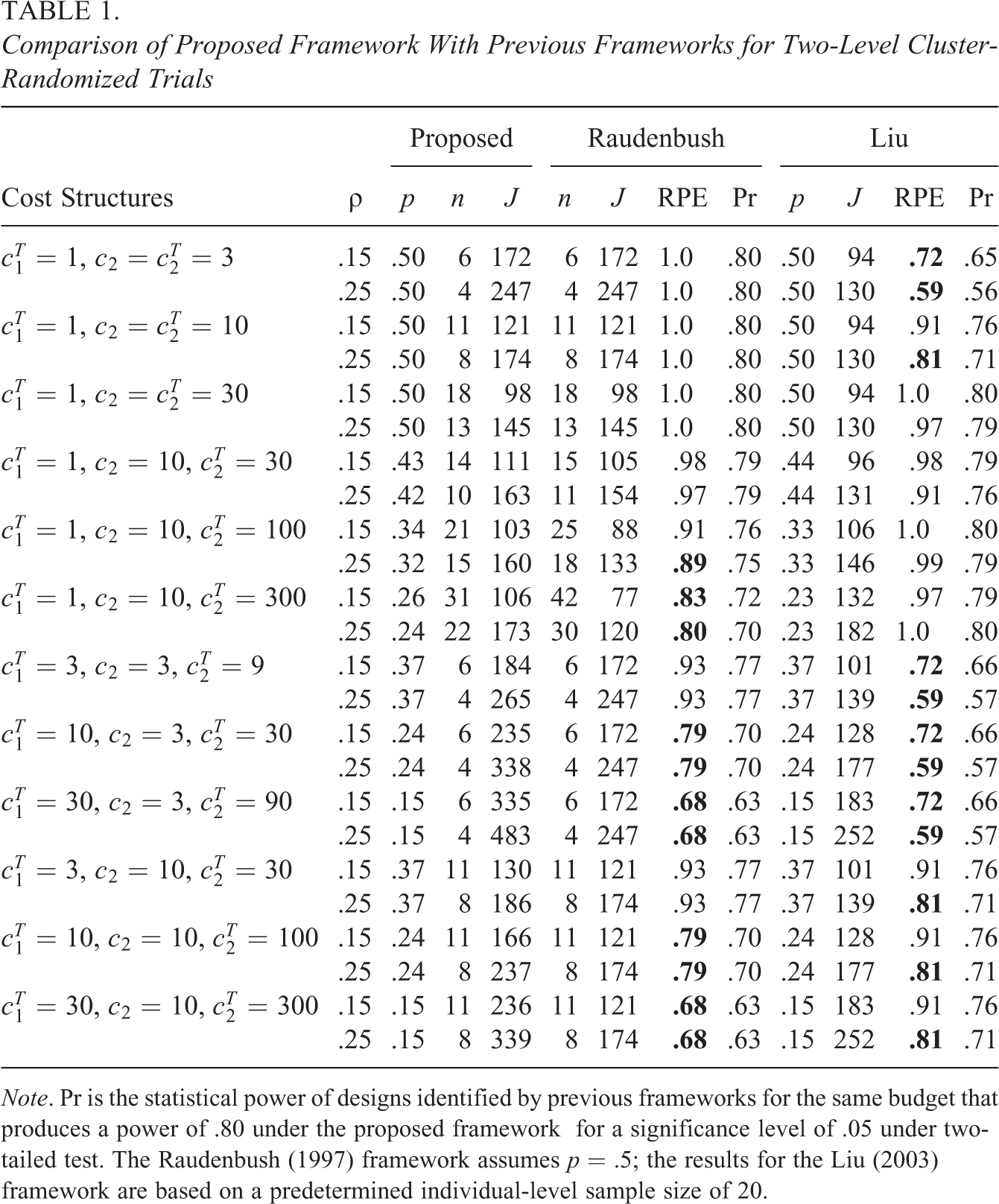
Note. Pr is the statistical power of designs identified by previous frameworks for the same budget that produces a power of .80 under the proposed framework for a significance level of .05 under two-tailed test. The Raudenbush (1997) framework assumes p = .5; the results for the Liu (2003) framework are based on a predetermined individual-level sample size of 20.

For the intraclass correlation coefficient, we considered values of 0.15 and 0.25 (e.g., Hedges & Hedberg, 2007). For the R squared values or the proportions of outcome variance explained by covariates, we considered three types of design. The first type of design has no covariate adjustment (i.e., $R_{1}^{2} = R_{2}^{2} = 0$ ). The second type of design has a half of cluster-level outcome variance explained by a cluster-level covariate (i.e., $R_{1}^{2} = 0$ , $R_{2}^{2} = 0.5$ , and $q = 1$ ). The third type of design has covariates explained a half of outcome variances at both the cluster and individual levels (i.e., $R_{1}^{2} = R_{2}^{2} = 0.5$ , and $q = 1$ ).

For simplicity, we used $n = 20$ as the predetermined individual-level sample size in the framework by Liu (2003). In the computation, we rounded the values of n to integers and the values of p and RPE to two decimal places. The results for designs with a cluster-level covariate are presented in Table 1. For the other two types of design (i.e., designs without a covariate and designs with covariates at both levels), the conclusions are similar with those in Table 1 and are not repeatedly presented.

Across all values of cost structures and design parameters, there are 11 of 24 designs identified under the Raudenbush (1997) framework have RPE values below the good level of .90 (see bold RPE values in Table 1). From a relative precision perspective, designs identified under the Raudenbush (1997) framework achieve lower statistical power under the same budgets requested by the proposed framework. The statistical power drops to .70 when the treatment/control sampling cost ratio is 10, and .63 for a cost ratio of 30 (Table 1). Half (12 of 24) of the designs identified under the Liu (2003) framework have RPE values below the good level of .90 (see the bold values in Table 1).

For designs identified under previous frameworks, the RPE values and the relative statistical power are directly influenced by how far the constrained values depart from the optimal values in our proposed framework. For example, when the costs of sampling are equal between treatment conditions (e.g., first three cost structures in Table 1), the constrained p under the Raudenbush (1997) framework is equal to the optimal $p = .5$ in our framework; thus, the Raudenbush framework can identify identical designs with RPE values of one. When the constrained $p = .5$ departs far away from the optimal values, designs identified under the Raudenbush framework have much lower RPE values and statistical power (e.g., the last cost structure in Table 1).

We can see similar patterns for the Liu (2003) framework in Table 1; when the predetermined $n = 20$ is close to the optimal values under the proposed framework, the RPE values for designs under the Liu (2003) framework are close to one (e.g., the third to sixth cost structures in Table 1). When the predetermined individual-level sample sizes are far from the optimal values, we have much lower RPE values and statistical power (e.g., the first cost structures in Table 1). Collectively, the results comparing with previous frameworks show that the proposed framework can be used to significantly improve design precision and efficiency, especially when the cost of sampling a treatment unit is multiple times that for a control unit.

To illustrate the difference in the required total sample size under different optimal design framework, further suppose researchers plan to implement the cluster-randomized trials to detect a standardized effect of 0.2 (Spybrook et al., 2016). We reported the total number of clusters (J) needed to have a power level of 0.8 for the effect size of 0.2 in Table 1. The results show that we can sample more clusters under the proposed framework than those under the Raudenbush (1997) framework but with less budget required to achieve a power of 0.8 (e.g., see J and RPE values for the forth to last cost structures in Table 1).

Comparing with the Raudenbush (1997) framework, the proposed framework gains efficiency mainly through sampling less clusters in the experimental group but much more clusters in the control group. This mechanism results in the opposite directions in the change of the optimal proportions p and the number of total clusters J. For example, comparing results in the first and last three cost structures in Table 1, we can clearly see that the more expensive sampling in treatment is, the smaller the optimal p and the larger the number of total clusters J. This mechanism of opposite directions in the change of p and J ensures that we still have enough clusters (e.g., classrooms) in the treatment condition.

For example, in the last cost structure where sampling a treatment cluster (e.g., regular class assisted by a teacher aide; Mosteller, 1995) costs 30 times that of sampling a cluster in control (e.g., a regular class), with $ρ = .25$ we need to sample 87 clusters in each treatment condition under the Raudenbush (1997) framework. However, under the proposed framework we have an optimal p of .15 and J of 339. The number of total clusters to be sampled is about twice the number in the balanced design (174). Under the proposed framework, there will be 51 clusters in the treatment condition, 36 clusters less than the balanced design, and 288 clusters in the control condition, 201 clusters more than the balanced design. Yet, the balanced design will require a 47% larger budget than the proposed framework to achieve comparable power.

Given the same requested budget by previous framework to detect an effect of 0.20 with a power of 0.8, we can detect a smaller effect under the proposed framework, and the MDES under proposed framework can be calculated based on these RPE values. Taking the same example mentioned above with an RPE of .68, we can detect an effect of 0.16 under the proposed framework with the same budget, which is 20% smaller than 0.20. The optimal sample allocation can improve design precision than that under the previous framework, and a smaller MDES can account for the overestimate of an effect size due to sampling error and other factors. In conclusion, we have shown that the proposed framework can be used to recover more gains in statistical precision and efficiency that have gone unconsidered in previous frameworks.

Design Sensitivity

To further probe the loss of efficiency resulting from constrained designs and the sensitivity of optimal designs to misspecifications of parameter values at the planning stage, we examined the extent to which proposed designs are robust to incorrect initial values of the cost structure and the design parameter values. Similarly, we only present the results for two-level cluster-randomized trials, as the conclusion is the same for three-level experiments.

In our analyses, we first calculated the true optimal design parameter values (n^o and p^o) based on the true values and then computed the optimal design parameter values (n and p) under misspecified initial values. Using Equation 31, we then computed the RPE value designs achieved. For the comparison, we used the same cost structures and design parameter values that have been used in the previous section. We rounded the values of n to integers and the values of p and RPE to two decimal places in the computation. We presented the result for designs with a covariate at the cluster level ( $R_{1}^{2} = 0$ and $R_{2}^{2} = .5$ ) in Table 2, results for other types of designs have similar conclusions and will be provided upon request.

Table 2.

Robustness of Optimal Sample Allocation to the Misspecification of Intraclass Correlation Coefficients

Cost Structures	$ρ$	Misspecification of $ρ$
Cost Structures	$ρ$	0.25	0.5	2	3
$c_{1}^{T} = 1$ , $c_{2} = c_{2}^{T} = 3$	.15	.89	.96	.97	.91
$c_{1}^{T} = 1$ , $c_{2} = c_{2}^{T} = 3$	.25	.88	.97	.88	.63
$c_{1}^{T} = 1$ , $c_{2} = c_{2}^{T} = 10$	.15	.87	.96	.96	.87
$c_{1}^{T} = 1$ , $c_{2} = c_{2}^{T} = 10$	.25	.86	.95	.90	.81
$c_{1}^{T} = 1$ , $c_{2} = c_{2}^{T} = 30$	.15	.88	.97	.96	.89
$c_{1}^{T} = 1$ , $c_{2} = c_{2}^{T} = 30$	.25	.87	.97	.95	.74
$c_{1}^{T} = 1$ , $c_{2} = 10$ , $c_{2}^{T} = 30$	.15	.87	.96	.95	.88
$c_{1}^{T} = 1$ , $c_{2} = 10$ , $c_{2}^{T} = 30$	.25	.86	.96	.93	.71
$c_{1}^{T} = 1$ , $c_{2} = 10$ , $c_{2}^{T} = 100$	.15	.87	.97	.95	.85
$c_{1}^{T} = 1$ , $c_{2} = 10$ , $c_{2}^{T} = 100$	.25	.87	.96	.95	.79
$c_{1}^{T} = 1$ , $c_{2} = 10$ , $c_{2}^{T} = 300$	.15	.89	.97	.96	.87
$c_{1}^{T} = 1$ , $c_{2} = 10$ , $c_{2}^{T} = 300$	.25	.89	.97	.95	.81
$c_{1}^{T} = 3$ , $c_{2} = 3$ , $c_{2}^{T} = 9$	.15	.89	.96	.97	.91
$c_{1}^{T} = 3$ , $c_{2} = 3$ , $c_{2}^{T} = 9$	.25	.88	.97	.88	.63
$c_{1}^{T} = 10$ , $c_{2} = 3$ , $c_{2}^{T} = 30$	.15	.89	.96	.97	.91
$c_{1}^{T} = 10$ , $c_{2} = 3$ , $c_{2}^{T} = 30$	.25	.88	.97	.88	.63
$c_{1}^{T} = 30$ , $c_{2} = 3$ , $c_{2}^{T} = 90$	.15	.89	.96	.97	.91
$c_{1}^{T} = 30$ , $c_{2} = 3$ , $c_{2}^{T} = 90$	.25	.88	.97	.88	.63
$c_{1}^{T} = 3$ , $c_{2} = 10$ , $c_{2}^{T} = 30$	.15	.87	.96	.96	.87
$c_{1}^{T} = 3$ , $c_{2} = 10$ , $c_{2}^{T} = 30$	.25	.86	.95	.90	.81
$c_{1}^{T} = 10$ , $c_{2} = 10$ , $c_{2}^{T} = 100$	.15	.87	.96	.96	.87
$c_{1}^{T} = 10$ , $c_{2} = 10$ , $c_{2}^{T} = 100$	.25	.86	.95	.90	.81
$c_{1}^{T} = 30$ , $c_{2} = 10$ , $c_{2}^{T} = 300$	.15	.87	.96	.96	.87
$c_{1}^{T} = 30$ , $c_{2} = 10$ , $c_{2}^{T} = 300$	.25	.86	.95	.90	.81
Average		.88	.96	.94	.81

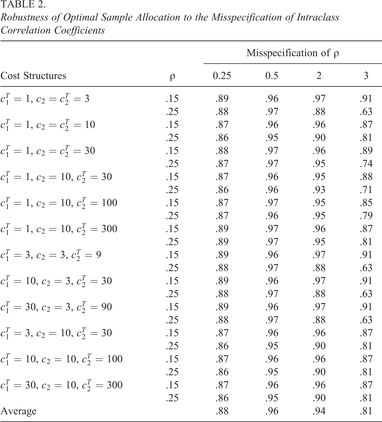
Robustness to the Misspecification of Intraclass Correlation Coefficient

In terms of the range of misspecification on intraclass correlation coefficient, we considered multiplicative values of the true parameter—0.25, 0.5, 2, and 3 times the true values—mapping the range of 0.25 to 2.75 times the true values within which constrained optimal designs ( $p = .5$ ) showed robustness in previous literature (Korendijk et al., 2010). Across cost structures, R squared values, and intraclass correlation coefficients, when the misspecification of intraclass correlation coefficients is 0.5 or 2 times the true values, designs averaged an RPE of .96 or .94, respectively (Table 2). Practically, the results suggest that planning studies under misspecifications of this type and magnitude will often require a budget that is only about 5% larger than the optimal design benchmark, or the optimal design can detect a less than 3% smaller effect.

When the misspecification of the intraclass correlation coefficient is even larger—for example, 0.25 or 3 times the true values—the average RPE values are about .88 and .81, respectively (Table 2). Our initial probe suggests that the optimal sample allocation identified under the proposed framework is fairly robust to the misspecification of the intraclass correlation coefficients.

Robustness to the Misspecification of Cost Structures

As for the misspecification of initial cost structure, we investigated the robustness of optimal design to the misspecification on initial CICR and TCCR. The range of the misspecification was set as 0.25, 0.5, 2, and 4 times the true values. The results are presented in Table 3. When the misspecification is 0.5 or 2 times the true CICR, designs have an average RPE value of .97. Even when the misspecification is 0.25 or 4 times the true CICR, designs have average RPE values of .89 or .90, respectively. As for the misspecification of initial TCCR values, the results are similar. Even when the misspecification is 0.25 or 4 times the true TCCRs, designs have an average RPE value of .90. The results suggest that designs optimized under moderate misspecifications of cost ratios largely retain their RPE values.

Table 3.

Robustness of Optimal Sample Allocation to Misspecification of Cost Structures Measured by Relative Precision and Efficiency

Cost Structures	$ρ$	Misspecification of CICR				Misspecification of TCCR
Cost Structures	$ρ$	0.25	0.5	2	4	0.25	0.5	2	4
$c_{1}^{T} = 1$ , $c_{2} = c_{2}^{T} = 3$	.15	.91	.97	.98	.89	.88	.97	.97	.88
$c_{1}^{T} = 1$ , $c_{2} = c_{2}^{T} = 3$	.25	.88	.97	.97	.91	.88	.97	.97	.88
$c_{1}^{T} = 1$ , $c_{2} = c_{2}^{T} = 10$	.15	.87	.98	.97	.89	.88	.97	.97	.88
$c_{1}^{T} = 1$ , $c_{2} = c_{2}^{T} = 10$	.25	.90	.95	.97	.90	.88	.97	.97	.88
$c_{1}^{T} = 1$ , $c_{2} = c_{2}^{T} = 30$	.15	.89	.97	.97	.89	.88	.97	.97	.88
$c_{1}^{T} = 1$ , $c_{2} = c_{2}^{T} = 30$	.25	.91	.97	.97	.90	.88	.97	.97	.88
$c_{1}^{T} = 1$ , $c_{2} = 10$ , $c_{2}^{T} = 30$	.15	.87	.97	.97	.88	.89	.97	.97	.88
$c_{1}^{T} = 1$ , $c_{2} = 10$ , $c_{2}^{T} = 30$	.25	.88	.96	.97	.89	.90	.97	.97	.89
$c_{1}^{T} = 1$ , $c_{2} = 10$ , $c_{2}^{T} = 100$	.15	.89	.97	.97	.89	.90	.97	.97	.90
$c_{1}^{T} = 1$ , $c_{2} = 10$ , $c_{2}^{T} = 100$	.25	.90	.97	.97	.91	.90	.98	.97	.90
$c_{1}^{T} = 1$ , $c_{2} = 10$ , $c_{2}^{T} = 300$	.15	.90	.97	.98	.90	.91	.98	.98	.90
$c_{1}^{T} = 1$ , $c_{2} = 10$ , $c_{2}^{T} = 300$	.25	.92	.98	.98	.91	.91	.98	.98	.89
$c_{1}^{T} = 3$ , $c_{2} = 3$ , $c_{2}^{T} = 9$	.15	.91	.97	.98	.89	.89	.97	.97	.89
$c_{1}^{T} = 3$ , $c_{2} = 3$ , $c_{2}^{T} = 9$	.25	.88	.97	.97	.91	.89	.97	.97	.89
$c_{1}^{T} = 10$ , $c_{2} = 3$ , $c_{2}^{T} = 30$	.15	.91	.97	.98	.89	.91	.98	.98	.92
$c_{1}^{T} = 10$ , $c_{2} = 3$ , $c_{2}^{T} = 30$	.25	.88	.97	.97	.91	.91	.98	.98	.92
$c_{1}^{T} = 30$ , $c_{2} = 3$ , $c_{2}^{T} = 90$	.15	.91	.97	.98	.89	.94	.98	.98	.93
$c_{1}^{T} = 30$ , $c_{2} = 3$ , $c_{2}^{T} = 90$	.25	.88	.97	.97	.91	.94	.98	.98	.93
$c_{1}^{T} = 3$ , $c_{2} = 10$ , $c_{2}^{T} = 30$	.15	.87	.98	.97	.89	.89	.97	.97	.89
$c_{1}^{T} = 3$ , $c_{2} = 10$ , $c_{2}^{T} = 30$	.25	.90	.95	.97	.90	.89	.97	.97	.89
$c_{1}^{T} = 10$ , $c_{2} = 10$ , $c_{2}^{T} = 100$	.15	.87	.98	.97	.89	.91	.98	.98	.92
$c_{1}^{T} = 10$ , $c_{2} = 10$ , $c_{2}^{T} = 100$	.25	.90	.95	.97	.90	.91	.98	.98	.92
$c_{1}^{T} = 30$ , $c_{2} = 10$ , $c_{2}^{T} = 300$	.15	.87	.98	.97	.89	.94	.98	.98	.93
$c_{1}^{T} = 30$ , $c_{2} = 10$ , $c_{2}^{T} = 300$	.25	.90	.95	.97	.90	.94	.98	.98	.93
Average		.89	.97	.97	.90	.90	.97	.97	.90

Note. CICR is the cluster/individual cost ratio. TCCR is the treatment/control cost ratio.

Discussion

Prior literature has developed a host of strategies and tools to improve the efficiency with which designs can estimate effects (e.g., Bloom et al., 2007; Borenstein et al., 2012; Dong & Maynard, 2013; Kelcey & Phelps, 2013; Kelcey et al., 2016; Schochet, 2008; Raudenbush et al., 2007). Previous optimal design frameworks have been limited in their modeling the cost structures of sampling and optimizing the sampling ratios across levels and treatment conditions. In this article, our proposed framework addresses this need by developing a flexible cost framework that more naturally maps onto practical design settings. The results of the extended framework identify potentially important gains in statistical precision and efficiency that have previously gone unconsidered.

Even when some of the parameters are constrained by practical considerations, our results suggest that within a broad range of applied settings the proposed framework can identify sampling strategies with more precision and efficiency than those detailed in previous literature. In this way, the introduction of a treatment-condition specific cost framework and the optimization of sampling ratios across levels and treatment conditions can be useful for adjudicating among several potential designs with varying constraints. Additionally, the proposed framework performed better than previous frameworks even when the parameter values are misspecified.

To design cluster-randomized trials with adequate statistical power and efficiency under an optimal design framework, researchers additionally need the cost information about sampling. The information about the cost of sampling a unit can usually be estimated through pilot studies, budget planning, similar studies, or cost centers (e.g., CostOut at https://www.cbcse.org/costout). Even when cost estimation may not be strictly accurate, our initial probe of the proposed optimal design framework suggested that the results are fairly robust to the misspecification on initial values of intraclass correlation coefficient and cost structures. In this way, our results suggest that even when some parameters are constrained, and some are misspecified, there are still advantages to probing more flexible sampling plans.

In the presence of unequal sampling costs between treatment conditions, we have illustrated that unbalanced designs can be more efficient than balanced ones. Put another way, unbalanced designs can return more statistical power than balanced designs under unequal sampling costs between treatment conditions. It is generally assumed that the treatment or intervention itself does not change the standardized variance of an outcome. For designs with unequal number of clusters between treatment conditions, the assumption of homogeneity of variance between treatment conditions (controlling for the treatment effect) can still be tested the same way with balanced designs as the variance formulas adjust for the number of clusters.

We illustrated the opposite directions in the change of the optimal p and the number of total clusters needed for a certain level of statistical power. This mechanism ensures that unbalanced designs still result in enough clusters to be sampled in a treatment condition. However, when the number of total clusters is small and the proportion of clusters to be assigned to the treatment condition is also small, there may be an issue whether the treatment arm can correctly reflect the population variance, and thus there may be a homoskedasticity issue between treatment conditions. Further studies address a small number of clusters in unbalanced design is needed.

Despite the utility of our framework and the potential gains in statistical precision and efficiency it offers, we caution readers that the resulting optimal sampling plans are intended to serve as a starting point for planning a cluster-randomized trial rather than a rigid tool. For example, an analysis of optimal design may suggest a small value of optimal proportion (p) if sampling costs are vastly different between treatment conditions. In power analysis, a small value of p may suggest a large number of total clusters that exceeds the clusters researchers could practically reach. In this case, researchers should constrain the optimal proportion to a larger number than that the analysis gives so that a feasible design can be achieved. In practice, the optimal sampling plan operates as a type of initial strategy or benchmark that is subsequently moderated by practical design considerations and constraints to reach a final sampling plan.

To facilitate end-user calculations, we have developed a freely available R package odr (Shen & Kelcey, 2020) that implements the proposed framework. The package also can perform power analysis accommodating costs by default (e.g., required budget/sample size calculation, power calculation under a given budget, MDES calculation under a given budget) and conventional power analysis (e.g., sample size, power, and MDES calculation).

Footnotes

Appendix A

Appendix B

Acknowledgments

We thank the editor, Dr. Daniel McCaffrey, three anonymous reviewers, and Dr. Luke Miratrix at Harvard University for their insightful comments and suggestions on earlier drafts of the manuscript.

Declaration of Conflicting Interests

The author(s) declared no potential conflicts of interest with respect to the research, authorship, and/or publication of this article.

Funding

The author(s) disclosed receipt of the following financial support for the research, authorship, and/or publication of this article: This article is based in part on work supported by the National Academy of Education (NAEd) and Spencer Foundation through a NAEd/Spencer Dissertation Fellowship awarded to the first author.

ORCID iD

Zuchao Shen

References

Bloom

H. S.

(1995). Minimum detectable effects: A simple way to report the statistical power of experimental designs. Evaluation Review, 19(5), 547–556.

Bloom

H. S.

(2005). Randomizing groups to evaluate place-based programs. In Bloom

H. S.

(Ed.), Learning more from social experiments: Evolving analytic approaches (pp. 115–172). Russell Sage Foundation.

Bloom

H. S.

Richburg-Hayes

Black

A. R.

(2007). Using covariates to improve precision for studies that randomize schools to evaluate educational interventions. Educational Evaluation and Policy Analysis, 29(1), 30–59.

Borenstein

Hedges

L. V.

Rothstein

(2012). CRT-power [Computer software]. Biostat. http://www.crt-power.com

Cochran

(1963). Sampling techniques (2nd ed.). Wiley.

Connelly

L. B.

(2003). Balancing the number and size of sites: An economic approach to the optimal design of cluster samples. Controlled Clinical Trials, 24(5), 544–559.

Dong

Maynard

R. A.

(2013). PowerUp!: A tool for calculating minimum detectable effect sizes and sample size requirements for experimental and quasi-experimental designs. Journal of Research on Educational Effectiveness, 6(1), 24–67.

Donner

Klar

(2000). Design and analysis of cluster randomization trials in health research. Arnold.

Glynn

T. J.

Shopland

D. R.

Manley

Lynn

W. R.

Freedman

L. S.

Green

S. B.

Corle

D. K.

Graubard

Baker

Mills

S. L.

Chapelsky

D. A.

Gail

Mark

Bettinghaus

Orlandi

M. A.

McAlister

Royce

Lewit

Dalton

L. T.

(1995). Community intervention trial for smoking cessation (COMMIT): I. Cohort results from a four-year community intervention. American Journal of Public Health, 85(2), 183–192.

10.

Greenleaf

C. L.

Litman

Hanson

T. L.

Rosen

Boscardin

C. K.

Herman

Schneider

S. A.

Madden

Jones

(2011). Integrating literacy and science in biology: Teaching and learning impacts of reading apprenticeship professional development. American Educational Research Journal, 48(3), 647–717.

11.

Hedges

L. V.

Borenstein

(2014). Conditional optimal design in three-and four-level experiments. Journal of Educational and Behavioral Statistics, 39(4), 257–281.

12.

Hedges

L. V.

Hedberg

E. C.

(2007). Intraclass correlation values for planning group-randomized trials in education. Educational Evaluation and Policy Analysis, 29(1), 60–87.

13.

Hiscock

Bayer

J. K.

Price

Ukoumunne

O. C.

Rogers

Wake

(2008). Universal parenting programme to prevent early childhood behavioural problems: Cluster randomised trial. British Medical Journal, 336(7639), 318–321.

14.

Hoover

D. R.

(2002). Power for T-test comparisons of unbalanced cluster exposure studies. Journal of Urban Health, 79(2), 278–294.

15.

Jacob

Goddard

Kim

Miller

Goddard

(2015). Exploring the causal impact of the McREL Balanced Leadership Program on leadership, principal efficacy, instructional climate, educator turnover, and student achievement. Educational Evaluation and Policy Analysis, 37(3), 314–332.

16.

Jayanthi

Gersten

Taylor

M. J.

Smolkowski

Dimino

(2017). Impact of the developing mathematical ideas professional development program on grade 4 students’ and teachers’ understanding of fractions (REL 2017–256). U.S. Department of Education, Institute of Education Sciences, National Center for Education Evaluation and Regional Assistance, Regional Educational Laboratory Southeast. http://ies.ed.gov/ncee/edlabs

17.

Kelcey

Phelps

(2013). Strategies for improving power in school-randomized studies of professional development. Evaluation Review, 37(6), 520–554.

18.

Kelcey

Shen

Spybrook

(2016). Intraclass correlation coefficients for designing cluster-randomized trials in sub-Saharan Africa education. Evaluation Review, 40(6), 500–525.

19.

Konstantopoulos

(2009). Incorporating cost in power analysis for three-level cluster-randomized designs. Evaluation Review, 33(4), 335–357.

20.

Konstantopoulos

(2011). Optimal sampling of units in three-level cluster randomized designs: An ANCOVA framework. Educational and Psychological Measurement, 71(5), 798–813.

21.

Korendijk

E. J.

Moerbeek

Maas

C. J.

(2010). The robustness of designs for trials with nested data against incorrect initial intracluster correlation coefficient estimates. Journal of Educational and Behavioral Statistics, 35(5), 566–585.

22.

Liu

(2003). Statistical power and optimum sample allocation ratio for treatment and control having unequal costs per unit of randomization. Journal of Educational and Behavioral Statistics, 28(3), 231–248.

23.

Moerbeek

van Breukelen

G. J.

Berger

M. P.

(2000). Design issues for experiments in multilevel populations. Journal of Educational and Behavioral Statistics, 25(3), 271–284.

24.

Mosteller

(1995). The Tennessee study of class size in the early school grades. The Future of Children, 5(2), 113–127.

25.

Nam

J. M.

(1973). Optimum sample sizes for the comparison of the control and treatment. Biometrics, 29, 101–108.

26.

Raudenbush

S. W.

(1997). Statistical analysis and optimal design for cluster randomized trials. Psychological Methods, 2(2), 173–185.

27.

Raudenbush

S. W.

Bryk

A. S.

(2002). Hierarchical linear models: Applications and data analysis methods (2nd ed.). Sage.

28.

Raudenbush

S. W.

Martinez

Spybrook

(2007). Strategies for improving precision in group-randomized experiments. Educational Evaluation and Policy Analysis, 29(1), 5–29.

29.

R Core Team. (2019). R: A language and environment for statistical computing [Software]. https://www.R-project.org/

30.

Rutterford

Copas

Eldridge

(2015). Methods for sample size determination in cluster randomized trials. International Journal of Epidemiology, 44(3), 1051–1067.

31.

Schochet

P. Z.

(2008). Statistical power for randomized assignment evaluation of education programs. Journal of Educational and Behavioral Statistics, 33(1), 62–87.

32.

Shen

Kelcey

(2020). odr: Optimal design and statistical power of multilevel randomized trials (Version 1.0.2) [Software]. Available from https://cran.r-project.org/web/packages/odr.

33.

Springer

M. G.

Ballou

Hamilton

V. N.

Lockwood

J. R.

McCaffrey

D. F.

Pepper

Stecher

B. M.

(2011). Teacher pay for performance: Experimental evidence from the Project on Incentives in Teaching (POINT). Society for Research on Educational Effectiveness. https://files.eric.ed.gov/fulltext/ED518378.pdf

34.

Spybrook

Shi

Kelcey

(2016). Progress in the past decade: An examination of the precision of cluster randomized trials funded by the US Institute of Education Sciences. International Journal of Research & Method in Education, 39(3), 255–267.

35.

Turner

R. M.

Toby Prevost

Thompson

S. G.

(2004). Allowing for imprecision of the intracluster correlation coefficient in the design of cluster randomized trials. Statistics in Medicine, 23(8), 1195–1214.