Coherent Power Analysis in Multilevel Studies Using Parameters From Surveys

Abstract

Researchers designing multisite and cluster randomized trials of educational interventions will usually conduct a power analysis in the planning stage of the study. To conduct the power analysis, researchers often use estimates of intracluster correlation coefficients and effect sizes derived from an analysis of survey data. When there is heterogeneity in treatment effects across the clusters in the study, these parameters will need to be adjusted to produce an accurate power analysis for a hierarchical trial design. The relevant adjustment factors are derived and presented in the current article. The adjustment factors depend upon the covariance between treatment effects and cluster-specific average values of the outcome variable, illustrating the need for better information about this parameter. The results in the article also facilitate understanding of the relative power of multisite and cluster randomized studies conducted on the same population by showing how the parameters necessary to compute power in the two types of designs are related. This is accomplished by relating parameters defined by linear mixed model specifications to parameters defined in terms of potential outcomes.

Keywords

power analysis experimental design hierarchical linear modeling

Recent years have seen an increased interest in the conduct of randomized experiments to evaluate the causal effects of educational policies and practices in the United States (Angrist, 2004; Spybrook, Cullen, & Lininger, 2011). This interest has been driven in large part by the Institute of Education Sciences (IES), which was created in 2002 and has made funding randomized experiments a priority (Constas, 2007; Whitehurst, 2004). The design of these experiments typically utilizes the hierarchical structure of the U.S. educational system (students are nested in classrooms, classrooms are nested in schools, schools are nested in districts, etc.).

Most experiments in education research can be thought of as variants of one of the two basic experimental designs. A cluster randomized or hierarchical trial randomly assigns entire groups of students to a treatment or control condition. For instance, entire schools may be randomly assigned. A randomized block or multisite trial utilizes groups of students as blocks in the experimental design. For instance, students within a given school may be randomly assigned in equal proportions to an experimental or control condition.

A key consideration when planning an experiment is the determination of the appropriate sample size. When the population being studied has a hierarchical structure, this involves making sample size determinations for each relevant level in the hierarchy (i.e., number of schools and number of students per school). The most common approach to sample size determination is to conduct a power analysis. For instance, many U.S. federal grant-making agencies, such as IES, require a power analysis to determine the appropriate sample size to use in a randomized experiment (National Center for Education Research, 2015).

Power analysis involves the specification of a statistical procedure that will be used to test the null hypothesis of a zero average treatment effect in the experiment. Sample sizes are chosen to ensure that Type I and Type II error rates for this test will be no higher than prespecified values. Statistical power is defined as 1 minus the Type II error rate. The Type I error rate is typically set to 0.05 (the usual level for “statistical significance”), and the Type II error rate is typically set to 0.20 (power of 0.80; e.g., Hedges & Rhoads, 2009; Schochet, 2008; Spybrook, Hedges, & Borenstein, 2014).

The usual approach to the analysis of cluster randomized and multisite experiments in education has been to utilize linear mixed models (linear regression models with both fixed and random effects) to account for the nesting of students within classrooms, schools, and/or districts. The parameters necessary to compute statistical power for hierarchical and multisite randomized trials can be defined in terms of the same linear mixed models used for statistical analysis (e.g., Raudenbush, 1997; Raudenbush & Liu, 2000; Spybrook et al., 2014). It is certainly appropriate to define parameters in this fashion, since a power analysis should be matched to the statistical procedure used to test the null hypothesis of no average treatment effect.

The current article argues for a subtle but important shift in how researchers approach the problem of power analysis for multisite and cluster randomized studies. The current approach to power analysis uses parameters that are defined in terms of quantities that can be observed and estimated for the design under consideration (e.g., Schochet, 2008; Spybrook et al., 2014). However, these may not be the most natural parameters to contemplate from the standpoint of design. To fully understand experimental design in multilevel settings, it is useful to define important quantities in terms of potential outcomes, some of which will be counterfactual in any given experiment (Rubin, 1974). This approach has proved fruitful for clarifying assumptions in many areas of statistics (e.g., Angrist, Imbens, & Rubin, 1996; Rosenbaum and Rubin, 1983), and it will prove to be no less fruitful here.

Conceptualizing hierarchical and multisite designs in terms of potential outcomes has three important benefits. First, it allows researchers to understand how the parameters that define power for a hierarchical design relate to the parameters that define power for a multisite design. This is important for the researcher who needs to decide whether it would be preferable to conduct a multisite trial or a hierarchical trial. It is well known that, all other things equal, multisite trials result in higher statistical power than hierarchical trials (Raudenbush, 1997; Raudenbush & Liu, 2000; Rhoads, 2011). However, there may be considerations other than power that would lead a researcher to opt for a hierarchical design (Rhoads, 2011). These include preferences of schools that will partner in the study, logistical or financial concerns (staff necessary to implement the experimental condition may be limited), and concerns about contamination in the multisite design (when there are students in the same school in both the experimental control conditions, students may be exposed to intervention elements intended for the opposite condition). When design decisions must be made based on both statistical and extrastatistical considerations, it is useful to understand how power in the multisite and hierarchical designs compare when a common set of assumptions is made for the respective power analyses.

The second important benefit of the potential outcomes approach is that it makes transparent the role of heterogeneity of treatment effects across clusters in determining power for both hierarchical and multisite designs. Since this heterogeneity cannot be estimated in hierarchical designs, researchers planning hierarchical studies using parameters defined in terms of observable quantities are likely to ignore heterogeneity in the planning process. Results presented in the article illustrate that failing to account for treatment effect heterogeneity when planning a hierarchical study can lead to very inaccurate estimates of the required sample size.

The third benefit of the potential outcomes approach, related to the second, is that it makes clear how to use parameters computed from surveys to inform the design of hierarchical studies. Parameters from surveys will need to be adjusted before being used in a power analysis. The adjustment is necessary because parameters computed from surveys will not be influenced by heterogeneity of treatment effects, whereas the parameters necessary for planning hierarchical experiments necessarily are influenced by heterogeneity in treatment effects.

In the interest of ensuring a simple exposition of the basic ideas, the article focuses exclusively on balanced designs with continuous outcomes. It also discusses only the relatively simple case where there is a single level of nesting. To fix ideas, it is assumed that the units under study involve students nested within schools. While details are provided only for this simple case, the logic of the argument applies to situations where units besides students and schools define the nesting structure as well as to more complex experimental designs with multiple levels of nesting.

The rest of this article proceeds as follows. The first section presents the standard linear mixed models used for the analysis of (1) a two-level hierarchical trial where students are nested in schools and schools are randomized and (2) a two-level multisite trial where students are randomized within schools. This section also presents the distributions of the test statistics used to compute power for each design. The second section presents models that represent the structure of the data under two potential states of the world: one where all schools and students receive the experimental treatment and the other where all schools and students receive the control treatment. This section then derives the variance of the estimator of the average treatment effect for each design in terms of these “potential outcomes” (Rubin, 1974). Parameters that characterize variance in terms of potential outcomes are compared to the standard parameterizations of the linear mixed model for hierarchical and multisite designs, revealing the connections between the commonly defined parameters for these two designs. In particular, the role that heterogeneity of treatment effects across schools plays in defining the variance function for each design is revealed. The third section discusses the ways researchers can determine the appropriate values to use in a power analysis and reviews the literature on empirical estimates of design parameters in education research. The fourth section shows when and how estimates of design parameters obtained from prior data (including surveys and prior experimental studies) should be adjusted to account for treatment effect heterogeneity before being used in a power analysis. The fifth section provides some illustrative values of the adjustment factors derived in the previous section and shows how treatment effect heterogeneity can influence the sample size required to achieve a desired power level. The sixth section provides illustrative power calculations both with and without the adjustment factors derived in the article. The final section contains some concluding remarks.

Linear Mixed Models for the Analysis of Two-Level Multisite and Hierarchical Studies

The Model for the Hierarchical Design

The usual linear mixed model used for the analysis of a two-level hierarchical trial is specified as follows. Assume a total of m schools, each containing 2n students, participate in the study. Let $Y_{i j k}^{H}$ be the value of the outcome variable for the kth student in the jth school in the ith treatment group. Assume that the distribution of the outcome variable is described by the following model:

Y_{i j k}^{H} = μ + α_{i} + β_{j (i)} + ∊_{i j k} .

The α _i parameters are fixed effects representing the deviation of the average score in the ith treatment group from the grand mean, the β _j _(i) parameters are independent, normally distributed random effects with variance τ_H and the ε _ijk parameters are independent, normally distributed random effects with variance $σ_{H}^{2}$ . Define the total variance in the outcome measure for the hierarchical design as $\sum_{H} = τ_{H} + σ_{H}^{2}$ . Define the intracluster correlation coefficient (ICC) for the hierarchical design (denoted ρ _H ) as follows:

ρ_{H} = \frac{τ_{H}}{\sum_{H}} .

The ICC quantifies proportion of the total variation in the outcome variable that is accounted for at the second level of the hierarchy. In other words, the total variation is partitioned into variation in student scores around a school mean and variation in school means about a grand mean. The ICC represents the proportion of the total variation that is accounted for by variation of the school means about the grand mean.

Denote the average value of the outcome variable in the experimental group by $Y_{_{E • •}}^{H}$ and the average value in the control group by $Y_{_{C • •}}^{H}$ . Similarly, denote the population average value of the outcome if everyone were to receive the experimental treatment as μ _E and denote the population average value of the outcome if everyone were to receive control as μ _C . It is well known (e.g., Raudenbush, 1997) that the model in Equation 1 implies

Var (Y_{E • •}^{H} - Y_{C • •}^{H}) = \frac{2}{m n} (σ_{H}^{2} + 2 n τ_{H}) = \frac{2}{m n} \sum_{H} (1 + (2 n - 1) ρ_{H}),

and that $Y_{E • •}^{H} - Y_{C • •}^{H}$ divided by its standard error has a noncentral t-distribution with m − 2 degrees of freedom and noncentrality parameter

λ_{h} = \frac{μ_{E} - μ_{c}}{\sqrt{\sum_{H}}} \sqrt{\frac{m n}{2}} \sqrt{\frac{1}{1 + (2 n - 1) ρ_{H}}} .

Power is typically computed using the distribution function of a noncentral t after specifying m, n, ρ _H , and the effect size, $δ_{H} = \frac{μ_{E} - μ_{c}}{\sqrt{\sum_{H}}}$ . For instance, the software programs CRT Power (Borenstein, Hedges, & Rothstein, 2012) and Optimal Design Plus (OD Plus, Raudenbush et. al., 2011) compute power in this manner after prompting the user to enter these parameters.

The Model for the Multisite Design

The usual linear mixed model used for the analysis of a two-level multisite trial is specified as follows. Again assume a total of m schools, each containing 2n students, participate in the study. Let $Y_{i j k}^{M}$ be the kth observation in the jth school in the ith treatment group, then

Y_{i j k}^{M} = μ + α_{i} + γ_{j} + {(α γ)}_{i j} + ε_{i j k} .

The α _i parameters are fixed effects representing the deviation of the average score in the ith treatment group from the grand mean, the γ _j parameters are independent, normally distributed random effects with variance τ_M, the (αγ) _ij parameters are independent, normally distributed random effects with variance ζ/2, and the ε _ijk parameters are independent, normally distributed random effects with variance $σ_{M}^{2}$ .

The variance of the (αγ) _ij parameters is written as ζ/2 because the variance in treatment effects across schools is Var{(αγ) _Ej − (αγ) _Cj } = 2 × Var{(αγ) _ij }. Therefore, ζ is the variance in treatment effects across schools.

It is well known (e.g., Raudenbush & Liu, 2000) that the model described in Equation 5 implies

Var (Y_{E • •}^{M} - Y_{C • •}^{M}) = \frac{2}{m n} (σ_{M}^{2} + n ζ / 2),

and $Y_{E • •}^{M} - Y_{C • •}^{M}$ divided by its standard error has a t-distribution with m − 1 degrees of freedom and noncentrality parameter

λ_{M} = \sqrt{\frac{m n}{2}} \frac{μ_{E} - μ_{c}}{\sqrt{σ_{M}^{2} + n ζ / 2}} .

The literature on statistical power in multisite designs contains different suggestions regarding the best way to rewrite Equation 7 in order to obtain interpretable parameters for use in a power analysis. For instance, the software programs CRT Power and OD Plus use different sets of parameters to compute power for a multisite design.

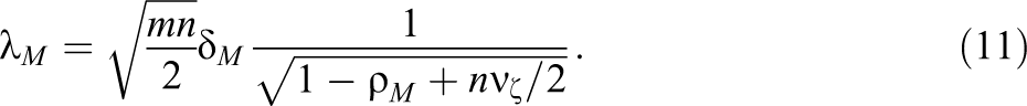
For reasons that will become clear in the next two sections, I argue that the following set of parameter definitions is most useful for computing power in the multisite design. Each definition involves standardizing one of the quantities in Equation 7 by the total variation in the outcome measure in the control group (or by the square root of that total variation). Using notation that is defined more completely in the next section, I make the following parameter definitions. The effect size, δ _M , is defined as

δ_{M} = \frac{μ_{E} - μ_{c}}{\sqrt{σ_{C}^{2} + τ_{C}}} .

The school-level ICC, ρ _M, is defined as

ρ_{M} = \frac{τ_{C}}{τ_{C} + σ_{C}^{2}} .

The standardized variance in treatment effects across schools, ν_ζ, is defined as

ν_{ζ} = \frac{ζ}{τ_{C} + σ_{C}^{2}} .

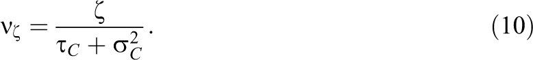
Using these definitions, we can rewrite the noncentrality parameter, λ_M, as

λ_{M} = \sqrt{\frac{m n}{2}} δ_{M} \frac{1}{\sqrt{1 - ρ_{M} + n ν_{ζ} / 2}} .

Interpreting Parameters Using Potential Outcomes

As noted in the introductory section, it is useful to define models that describe the distribution of the outcome variable under two contrasting hypothetical worlds. In one world, all schools and students receive the control condition. In the other world, they all receive the experimental condition. This way of defining potential outcomes is often referred to as Rubin’s causal model (Holland, 1986). Writing models in terms of potential outcomes clarifies the relationship between the parameters commonly used to compute power in hierarchical and multisite trials. It also illustrates the role that treatment effect heterogeneity plays in the computation of power. Finally, the potential outcomes approach helps make clear how parameters estimated from surveys may be used to help plan multisite and hierarchical experiments.

Thus, in this section, we assume that the following model describes the outcome that would be observed for the kth student in the jth school in the hypothetical world where everyone was assigned to the control condition:

Y_{j k}^{C} = μ_{c} + β_{j}^{C} + ε_{j k}^{C}, j = 1, …, m; k = 1, …, 2 n .

On the other hand, in the hypothetical world where everyone was assigned to the experimental condition, the distribution of the outcome variable would follow the following model:

Y_{j k}^{E} = μ_{E} + β_{j}^{E} + ε_{j k}^{E}, j = 1, …, m; k = 1, …, 2 n .

$β_{j}^{C} (β_{j}^{E})$ is a mean zero, normally distributed random effect having variance $τ_{C} (τ_{E})$ and representing the deviation of the mean outcome in school j under treatment regime C (E) from the overall population mean under treatment regime C (E). Also, $ε_{j k}^{C} (ε_{j k}^{E})$ is a mean zero, normally distributed random effect associated with individual k within school j that represents the deviation of the individual’s score from the school mean under treatment regime C (E) and has variance $σ_{C}^{2} (σ_{E}^{2})$ . It is more useful to think of the school-level random effect in the experimental group as a function of the school-level random effect in the control group plus a randomly varying treatment effect. Thus, write

β_{j}^{E} = β_{j}^{C} + δ_{j} .

The δ _j are the school-specific treatment effects with variance ζ. Define covariance between the school-specific treatment effects and school-level random effects in the control group as follows:

cov (β_{j}^{C}, δ_{j}) = κ .

Using the definition in Equation 13 in conjunction with Equation 12 gives the following relationship:

τ_{E} = τ_{C} + ζ + 2 κ .

For the purposes of computing power, it will be useful to define a standardized version of the κ parameter. Just as ζ was standardized by defining $ν_{ζ} = \frac{ζ}{τ_{C} + σ_{C}^{2}}$ , κ is standardized by defining

ν_{κ} = \frac{κ}{τ_{C} + σ_{C}^{2}} .

The experimental estimate of the population average treatment effect is given by

\hat{TE} = \sum_{j = 1}^{m} \sum_{k = 1}^{2 n} \frac{Z_{j k}}{m n} .

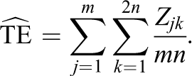
Z_jk is defined by $Z_{j k} = Y_{j k}^{E} (I_{j k}) - Y_{j k}^{C} (1 - I_{j k})$ , where I_jk = 1 if subject k in cluster j is assigned to the experimental condition and 0 otherwise. Thus, the I_jks are Bernoulli distributed random variables indicating treatment assignment. Of course, the I_jks have different distributions for hierarchical and multisite trials.

The variance of the treatment effect estimate, $Var (\hat{TE})$ , can be computed using the law of total covariance, the law of iterated expectations, and the law of total variance (see, e.g., Casella & Berger, 2002, p. 167). Details are provided in the Appendix (available in the online version of the journal). Define $σ_{a v}^{2} = \frac{σ_{C}^{2} + σ_{E}^{2}}{2}$ and $τ_{a v} = \frac{τ_{C} + τ_{E}}{2}$ . Then the variance of the treatment effect estimate for the hierarchical design can be written as

{Var}_{HT} (\hat{TE}) = \frac{2}{m n} [σ_{a v}^{2} + 2 n (τ_{a v})] .

The variance of the treatment effect estimate for the multisite design can be written as

{Var}_{MST} (\hat{TE}) = \frac{2}{m n} [σ_{a v}^{2} + (n ζ) / 2] .

Comparing the expressions in Equations 16 and 17 with the corresponding variance expressions in Equations 3 and 6 gives the following equations.

\frac{2}{m n} [σ_{H}^{2} + 2 n (τ_{H})] = \frac{2}{m n} [σ_{a v}^{2} + 2 n (τ_{a v})] .

\frac{2}{m n} [σ_{M}^{2} + n ζ / 2] = \frac{2}{m n} [σ_{a v}^{2} + n ζ / 2] .

Examination of Equations 18 and 19 reveals the following facts. First, the within-school variance components in the hierarchical and multisite designs have the same interpretation and can be interpreted as the average variance within schools across the two potential treatment regimes ( $σ_{M}^{2} = σ_{H}^{2} = σ_{a v}^{2}$ ). Second, the between-school variance component in the hierarchical design is really an average of the between-school variance in the experimental group and the between-school variance in the control group (τ_H = τ_av). Equation 14 makes clear that the between-school variance in the experimental group (τ_E) depends on (1) the between-school variance in the control group (τ_C), (2) the variance in treatment effects across schools (ζ), and (3) the covariance between school means in the control group and school-specific treatment effects (τ_κ). It follows that the ICC necessary to compute power in the hierarchical design (ρ_H) also depends on these three quantities.

Existing Empirical Work to Determine Design Parameters for Education Research

Because estimates of ICCs (like ρ_H or ρ_M), effect sizes (like δ_H or δ_M), and effect size variances (like ζ or ν_ζ) are necessary to plan experiments, they are sometimes referred to as “design parameters.” Since previous work has not recognized the importance of understanding the covariance between control group means and treatment effects, parameters such as κ and ν_κ have not been recognized as important design parameters. While κ and ν_κ can be estimated in multisite designs, researchers generally have not done so. However, there has been important empirical work in recent years that seeks to clarify the likely values of other design parameters for education research, including a recent special issue of the journal Evaluation Review (Spybrook, 2014). This section provides a brief summary of some of this empirical work. I consider in turn the literature on ICCs, work to determine likely values for the effect size parameter, and, finally, empirical estimates of effect size variances and related parameters.

Empirical Estimates of ICCs for Designs With Students Nested Within Schools

Hedges and Hedberg (2007a) published a widely used compendium of two-level ICCs for the case of students nested within schools. A variety of survey-based data sources providing nationally representative probability samples were used to compute ICCs for reading and math achievement for each grade level from K to 12. A companion paper by the same team provides similar estimates that are specific to rural schools (Hedges & Hedberg, 2007b). Hedges and Hedberg find that ICCs for students nested within schools are typically between 0.10 and 0.30. There is also a recently available “variance almanac” that allows researchers to obtain parameter estimates specific to a particular outcome variable type, region of the country, urbanicity, and grade level (Hedges & Hedberg, 2016).

Westine, Spybrook, and Taylor (2013) present two-level (students within schools) and three-level (students within schools within districts) ICCs using a longitudinal database and treating science, reading, and math achievement test scores as the outcome variable. Data come from the state of Texas. Brandon, Harrison, and Lawton (2013) present two-level ICC values (students within schools) using data on state reading assessments from the state of Hawaii. Xu and Nichols (2010) present both two-level (students within schools) and three-level ICC values (students within classrooms within schools) using statewide databases from Florida and North Carolina.

In each of the above papers, the ICCs estimated from two-level models using achievement test data were consistent with the range of values found in the earlier study by Hedges and Hedberg (2007a). Westine et al. (2013) obtain two-level ICCs ranging from 0.10 to 0.20. Brandon et al. (2013) also find two-level ICCs ranging from 0.10 to 0.20. ICCs computed in Xu and Nichols (2010) were between 0.09 and 0.13.

While there seems to be a growing consensus that school-based ICC values between 0.10 and 0.30 are reasonable when standardized achievement tests are the outcome measure, a very different picture emerges when the outcome measures are emotional and behavioral outcomes (such as measures of inattentiveness or hyperactivity) or health outcomes (such as “overweight status”). Jacob, Zhu, and Bloom (2010) present evidence that ICCs in these cases are quite low, ranging from 0 to 0.021 depending on the outcome measure.

Benchmark Effect Sizes for Educational Evaluations

Many in the social sciences are familiar with Cohen’s (1988) work in the area of statistical power and effect size. Cohen famously suggested labeling effect sizes of 0.20, 0.50, and 0.80 as “small,” “medium,” and “large,” respectively. Schochet (2008) notes that effect sizes between 0.20 and 0.33 have typically been used in educational evaluations. Bloom, Hill, Rebeck-Black, and Lipsey (2008) set out to provide a better empirical basis for determining what types of effect sizes are likely to exist for randomized trials evaluating educational interventions. Bloom et al. approach the problem by examining typical growth in vertically scaled educational tests. They used data from the national norming studies for six standardized tests in the domains of math, reading, science, and social studies to create “benchmark” effect sizes. Their results indicate that average annual growth in effect size units is much higher in the lower grades (e.g., 1st–3rd grade) relative to upper grades (e.g., 10th–12th grade). Growth in the lower grades could be as high as 1 standard deviation unit whereas growth in the upper grades is never higher than 0.25 standard deviations. Recent work by Scammacca, Fall, and Roberts (2015) has replicated the Bloom et al. (2008) study using a more recent norming sample and focusing attention on the bottom quartile of the normative distribution. These benchmarks may be more appropriate for interventions targeted to low-achieving or special education students.

Empirical Estimates of the Standardized Effect Size Variance

There is limited information in the literature about treatment effect heterogeneity. However, this section presents a brief summary of the information that is available. Unfortunately, even when estimates of ζ are reported, it can be hard to determine ν_ζ because estimates of the between-school variance in the control group are not generally available. In other instances, the value reported in the literature standardizes ζ by Σ _H . Unless information about κ is also reported, it is impossible to determine the value of ν_ζ. The estimates presented in the next paragraph have been computed using estimates of ζ reported from hierarchical linear model analyses and standardized by Σ _H . To the extent that Σ _H differs from $τ_{C} + σ_{C}^{2}$ , the true values of ν_ζ may be slightly different than those reported below.

Schochet (2008) discusses data from the evaluations of three programs: the 21st-Century Program, the School Dropout Demonstration Assistance Program, and Head Start. He reports values of ν_ζ between 0.04 and 0.08. Konstantopoulos (2008) reports a value of around 0.03 using data from Project STAR. Kosko and Miyazaki (2012) use data from the Early Childhood Longitudinal Study fifth grade to study the impact of mathematics discussion on math achievement in the fifth grade. They report variance component estimates that imply a ν_ζ value of 0.37. Kim et al. (2011) describe a study of the Pathway Project professional development intervention. The goal of the intervention is to improve analytical writing instruction for Latino English language learner students. Depending on the outcome measure utilized, ν_ζ values range from as low as 0 to as high as 0.66. Finally, Bloom and Weiland (2015) discuss variation in impacts across Head Start centers. Across six outcome measures studied, estimates of ν_ζ ranged from 0.005 to 0.063.

Another approach (Raudenbush & Liu, 2000) to determining plausible values of ν_ζ does not rely on empirical estimates, but rather considers the likely range of standardized treatment effects across the schools in the study. For instance, assume that school-specific (standardized) treatment effects roughly follow a normal distribution with a mean of 0.20 and that about 95% of school-specific treatment effects fall between 0 and 0.40. This would imply a standard deviation for school-specific treatment effects of 0.10 and a corresponding value of 0.01 for ν_ζ.

Raudenbush and Liu (2000) define a parameter $ν_{w} = \frac{ζ}{σ_{}^{2}}$ and use the above argument to label values of 0.05, 0.10, and 0.15 as “small,” “medium,” and “large,” respectively. Assuming an ICC parameter of about 0.20, this implies ν_ζ values of 0.04, 0.08, and 0.12 should be considered “small,” “medium,” and “large.”

Adjusting Design Parameters to Account for the Effects of Heterogeneity

The estimates of ICCs and benchmark effect sizes described in the previous section are valuable tools for educational researchers to use when planning experimental studies. However, because these ICC and effect size estimates are based on survey data and so do not account for treatment effect variance, they are not the correct ICC and effect size parameters to use when planning a hierarchical study. This section considers adjustments that can be made to survey-based ICCs and/or effect size benchmarks in order to produce an accurate power analysis for hierarchical designs. One can think of these adjustment factors as design effects (in the sense of Kish, 1965) that quantify the impact of treatment effect heterogeneity on a design.

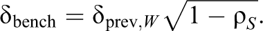
In addition to effect size benchmarks, another common way to determine an appropriate effect size to use when planning a research study is to utilize an estimate from a previous study of a similar experimental treatment. Depending on the previous study and how the effect size was computed, these estimates may also need to be adjusted in order to produce an accurate power analysis. In this case, adjustments may be necessary for both hierarchical and multisite designs. The necessary adjustment factors are derived later in this section.

In order to obtain tractable results for the relevant adjustment factors, this section assumes the individual-level variance is the same in the experimental and control groups ( $σ_{C}^{2} = σ_{E}^{2} = σ_{}^{2}$ ). This is consistent with current practice for power analyses of educational interventions, where variance in treatment effects across clusters is taken in to account (at least in multisite designs), but assumptions about variance in treatment effects at the individual level do not play a role. I also assume that the educational experiment will compare a novel educational intervention with a control group which will receive the “business as usual” educational practice for the schools under study.

The assumption of a business as usual control group implies that ICCs derived from surveys are estimating the ICC in the control group of the experiment. In other words,

ρ_{survey} = \frac{τ_{C}}{τ_{C} + σ_{}^{2}} = ρ_{M} .

In the following, we abbreviate ρ_survey by ρ_s.

Similarly, effect size benchmarks derived from surveys of educational performance can be assumed to represent business as usual for the population surveyed. As such, one can interpret an effect size benchmark (such as those presented in Bloom, Hill, Rebeck-Black, & Lipsey, 2008; or Scammacca, Fall, & Roberts, 2015) as a raw mean difference divided by the total standard deviation of the outcome measure in the control group. In other words,

δ_{bench} = \frac{μ_{E} - μ_{c}}{\sqrt{τ_{C} + σ_{}^{2}}} = δ_{M} .

It is immediately evident from Equations 20 and 21 that survey-based ICCs and effect size benchmarks are the appropriate parameters to use when planning a multisite study. Specification of these two parameters, along with the standardized effect size variance, ν_ζ, allows for the correct computation of power in a multisite design.

If an effect size estimate from a previous study is used to inform a power analysis, it is necessary to have some understanding of the context of the previous study in order to properly contextualize the estimate. In all cases, we must assume that the outcome measure used in the previous study is similar to the one being used in the present study. If the study was performed in a single school which is reasonably representative of the schools in the present study and the within-treatment group standard deviation was used to standardize the estimate, then the effect size may be written as

δ_{prev, W} = \frac{μ_{E} - μ_{c}}{σ} .

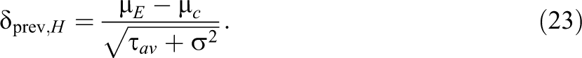
On the other hand, suppose the previous study involved multiple schools. In order to utilize the effect size estimate from this study for planning purposes, one must assume that the population of schools in the previous study is a reasonable approximation to the population of schools in the present study. If the previous study was a multisite study and the pooled within-school and within-treatment group standard deviation was used to standardize, then this estimate again corresponds to δ_prev,W. If the previous study was a hierarchical study and the total standard deviation was used to compute the effect size estimate, then

δ_{prev, H} = \frac{μ_{E} - μ_{c}}{\sqrt{τ_{a v} + σ_{}^{2}}} .

The next section considers how and when survey-based ICCs and/or effect size estimates should be adjusted to create an appropriate power analysis when planning an educational experiment.

Adjustments When Planning a Hierarchical Trial

Suppose that a researcher is planning a hierarchical trial using a survey-based ICC estimate. Below are adjustments that can be used when each of the three possible effect size estimates listed above (δ_prev,H, δ_bench, and δ_prev,W) are used to inform the power analysis.

Using δ_prev,H

Here the denominator of the effect size estimate is correct, so it is only necessary to adjust the survey-based ICC to convert it to the ICC relevant to the hierarchical experiment. We do this by multiplying ρ_s by a constant k_H, which satisfies the following equation:

k_{H} = \frac{ρ_{H}}{ρ_{S}} .

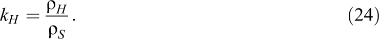
It is useful to see explicitly how k_H depends on treatment effect heterogeneity. Making the necessary substitutions and simplifying (see Appendix, available in the online version of the journal, for details) obtains the following expression for k_H :

k_{H} = \frac{1 + (ν_{ζ} / 2 + ν_{κ}) / ρ_{S}}{1 + (ν_{ζ} / 2 + ν_{κ})} .

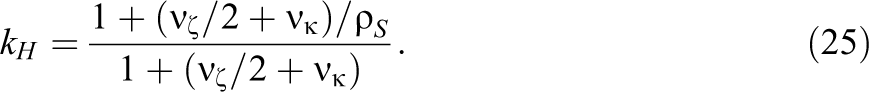
Let $ν_{T} = ν_{ζ} + 2 \times ν_{κ}$ represent the joint (standardized) effect of (a) treatment effect variance and (b) the covariance of treatment effects with control group means on variance in the experimental group. Then

k_{H} = \frac{2 + ν_{T} / ρ_{S}}{2 + ν_{T}} .

Clearly k_H is 1 when the ICC, ρ_S, is 1 or when there is no treatment effect heterogeneity. Also, the value of k_H approaches infinity, as ρ_S approaches zero for a fixed value of ν_τ.

It is possible to use properties of covariances and variances to derive bounds for the possible values of k_H . These bounds depend on ρ_S and ν_ζ but not ν_κ. Details of the derivation of the bounds are provided in the Appendix (available in the online version of the journal). The equation defining the bounds is

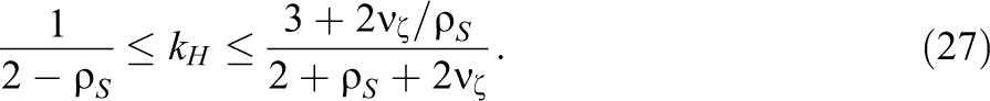
\frac{1}{2 - ρ_{S}} \leq k_{H} \leq \frac{3 + 2 ν_{ζ} / ρ_{S}}{2 + ρ_{S} + 2 ν_{ζ}} .

Equation 27 shows that the adjusted ICC can be lower than the unadjusted ICC. This occurs if the covariance between school-specific treatment effects and school-specific control group means is strongly negative. Conversely, the value of k_H will be greater than 1, provided that the covariance between school-specific treatment effects and school-specific control group means is either positive or weakly negative. Tables illustrating different values of k_H that result when different design parameters are specified are presented in the next section.

Using δ_bench

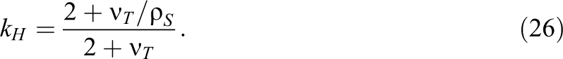
In this case, one needs to adjust for the effect of heterogeneity on the effect size denominator as well as its effect on the ICC. This can be accomplished by specifying a single, adjusted ICC. This involves multiplying ρ_s by a constant k_b which satisfies the following equation:

{1 + (2 n - 1) k_{b} ρ_{s}} (σ^{2} + τ_{C}) = 2 n τ_{a v} + σ^{2} .

A value of k_b satisfying this equation will ensure that the noncentrality parameter used for power calculations is equivalent to Equation 4. Performing some substitutions and algebraic manipulations (details provided in the Appendix, available in the online version of the journal) results in the following equation

k_{b} = 1 + \frac{n}{2 n - 1} (\frac{ν_{T}}{ρ_{S}}) .

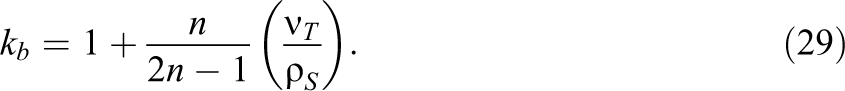
Of course, if there is no treatment effect heterogeneity (so ν_T = 0), then k_b =1 and ρ_S does not need to be adjusted.

It is also possible to derive bounds for the possible values for k_b . Derivations presented in the Appendix (available in the online version of the journal) show that

1 - \frac{n}{2 n - 1} \leq k_{b} \leq 1 + \frac{n}{2 n - 1} (\frac{2 ν_{ζ}}{ρ_{S}} + 1) .

Since $n / (2 n - 1) \approx 1 / 2$ for any reasonably large n, one can write the following approximate inequality:

\frac{1}{2} \leq k_{b} \leq \frac{3}{2} + (\frac{ν_{ζ}}{ρ_{S}}) .

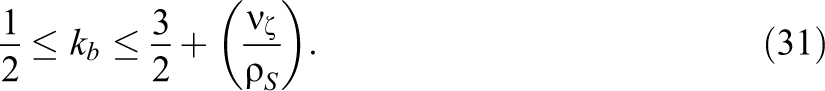
Again, it is clear that heterogeneity of treatment effects across schools can decrease the effective ICC if there is a strong negative covariance between treatment effects and the control group school means. However, if this covariance is positive or only weakly negative, k_b will be greater than 1 and heterogeneity of treatment effects will increase the effective ICC. Tables illustrating different values of k_b that result when different design parameters are specified are presented in the next section.

Using δ_prev,W

This case can be dealt with by simply converting δ_prev,W into δ_bench using the following identity:

δ_{bench} = δ_{prev, W} \sqrt{1 - ρ_{S}} .

The converted value of δ_prev,W and the value of k_b computed previously can then be used to adjust the ICC and perform the power analysis.

Adjustments When Planning a Multisite Trial

The current section considers adjustments to design parameters that may be necessary when planning a multisite trial.

Using δ_bench

The proposal to standardize parameters used when planning a multisite trial using the control group standard deviation was made precisely to simply computations in this case. Clearly, δ_bench = δ_M and ρ_S = ρ_M. Specification of these two parameters plus ν_ζ and the sample sizes at each level are all that is necessary to conduct the power analysis. Therefore, no adjustments need to be made.

Using δ_prev,W

This case can be dealt within the same fashion as in a hierarchical trial. Simply convert δ_prev,W into δ_bench using the following identity:

δ_{bench} = δ_{prev, W} \sqrt{1 - ρ_{S}} .

As noted above, the power analysis using δ_bench and ρ_S is correct without further adjustments.

Using δ_prev,H

In this case, there is unwanted heterogeneity in the denominator of the effect size estimate. It is easiest to adjust the effect size estimate in this case. The correct effect size to use is k_Mδ_prev,H, with k_M defined by

k_{M} = \sqrt{\frac{τ_{a v} + σ^{2}}{τ_{C} + σ^{2}}} .

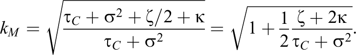
Substituting $(τ_{E} + τ_{C}) / 2$ for τ_av and the right-hand side of Equation 14 for τ_E results in the following expression for k_M:

k_{M} = \sqrt{\frac{τ_{C} + σ^{2} + ζ / 2 + κ}{τ_{C} + σ^{2}}} = \sqrt{1 + \frac{1}{2} \frac{ζ + 2 κ}{τ_{C} + σ^{2}}} .

Substituting ν_T for $\frac{ζ + 2 κ}{τ + σ^{2}}$ gives the following expression:

k_{M} = \sqrt{1 + ν_{T} / 2} .

Bounds for the correction factor are given in Equation 34 (details in the Appendix, available in the online version of the journal). These bounds are

\sqrt{1 - \frac{ρ_{S}}{2}} \leq k_{M} \leq \sqrt{1 + \frac{ρ_{S}}{2} + ν_{ζ}} .

Illustrations Using the Above Results

The tables and figures in this section present illustrative values of the adjustment factors just derived for different configurations of design parameters. This section also compares the required sample sizes that would be computed in a power analysis when design parameters are (incorrectly) utilized without adjustment to the sample sizes that result when the adjustment factors are used. Hierarchical designs are considered first and then multisite designs.

Illustrative Values of Adjustment Factors for Hierarchical Designs

Tables 1 and 2 present illustrative values of k_H and k_b, respectively. In light of the previous discussion regarding survey-based estimates of ICCs, illustrations are provided for both low ICC values (0.001, 0.01, and 0.05), which are likely to occur in studies with behavioral or health outcomes and for higher ICC values (0.10, 0.20, and 0.30), which are likely to occur in studies with academic achievement outcomes. The computations set the standardized variance in treatment effects across schools, ν_ζ, to 0.01, 0.05, 0.10, and 0.20. While some empirical estimates of ν_ζ larger than 0.20 are found in the literature, this would be considered a very large value of ν_ζ relative to the rules presented by Raudenbush and Liu (2000) and relative to most empirical estimates from larger studies (which should be more stable). The k_H factor does not depend on the within-school sample size (2n) but the k_b factor does. Computations for k_b assume a moderately sized value of n = 25.

Table 1.

Correction Factor (k_H ) When Planning a Hierarchical Study With a Survey-Based ICC and an Effect Size From a Previous Hierarchical Study (so Only the ICC Needs to Be Corrected)

		ρ _s
ν_ζ	ν_κ	0.001	0.01	0.05	0.1	0.2	0.3
0.01	LB	0.500	0.503	0.513	0.526	0.556	0.588
	LB/2	3.243	1.000	0.808	0.793	0.801	0.818
	0	5.970	1.493	1.095	1.045	1.020	1.012
	UB/2	8.683	1.980	1.373	1.283	1.217	1.178
	UB	11.381	2.463	1.643	1.509	1.396	1.322
0.05	LB	0.500	0.503	0.513	0.526	0.556	0.588
	LB/2	13.090	1.980	1.000	0.886	0.844	0.844
	0	25.366	3.415	1.463	1.220	1.098	1.057
	UB/2	37.340	4.808	1.905	1.529	1.322	1.236
	UB	49.024	6.161	2.326	1.818	1.522	1.389
0.1	LB	0.500	0.503	0.513	0.526	0.556	0.588
	LB/2	25.128	3.178	1.235	1.000	0.897	0.877
	0	48.571	5.714	1.905	1.429	1.190	1.111
	UB/2	70.914	8.121	2.529	1.818	1.444	1.304
	UB	92.231	10.407	3.111	2.174	1.667	1.467
0.2	LB	0.500	0.503	0.513	0.526	0.556	0.588
	LB/2	48.345	5.489	1.687	1.220	1.000	0.940
	0	91.818	10.000	2.727	1.818	1.364	1.212
	UB/2	131.493	14.100	3.656	2.340	1.667	1.429
	UB	167.847	17.842	4.490	2.800	1.923	1.605

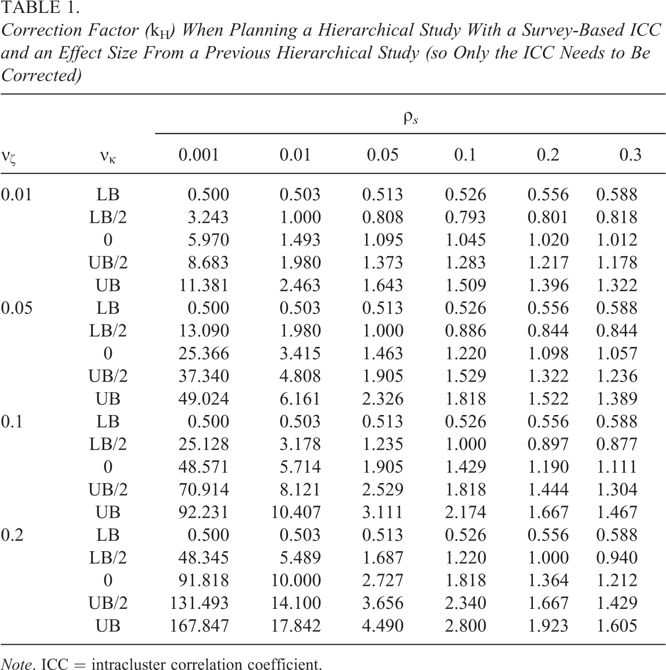
Note. ICC = intracluster correlation coefficient.

Table 2.

Correction Factor (k_b ) When Planning a Hierarchical Study With a Survey-Based ICC and a Benchmark Effect Size

		ρ _s
ν_ζ	ν_κ	0.001	0.01	0.05	0.1	0.2	0.3
0.01	LB	0.490	0.490	0.490	0.490	0.490	0.490
	LB/2	3.296	1.000	0.796	0.770	0.758	0.753
	0	6.102	1.510	1.102	1.051	1.026	1.017
	UB/2	8.908	2.020	1.408	1.332	1.293	1.281
	UB	11.714	2.531	1.714	1.612	1.561	1.544
0.05	LB	0.490	0.490	0.490	0.490	0.490	0.490
	LB/2	13.500	2.020	1.000	0.872	0.809	0.787
	0	26.510	3.551	1.510	1.255	1.128	1.085
	UB/2	39.520	5.082	2.020	1.638	1.446	1.383
	UB	52.531	6.612	2.531	2.020	1.765	1.680
0.1	LB	0.490	0.490	0.490	0.490	0.490	0.490
	LB/2	26.255	3.296	1.255	1.000	0.872	0.830
	0	52.020	6.102	2.020	1.510	1.255	1.170
	UB/2	77.786	8.908	2.786	2.020	1.638	1.510
	UB	103.551	11.714	3.551	2.531	2.020	1.850
0.2	LB	0.490	0.490	0.490	0.490	0.490	0.490
	LB/2	51.765	5.847	1.765	1.255	1.000	0.915
	0	103.041	11.204	3.041	2.020	1.510	1.340
	UB/2	154.316	16.561	4.316	2.786	2.020	1.765
	UB	205.592	21.918	5.592	3.551	2.531	2.190

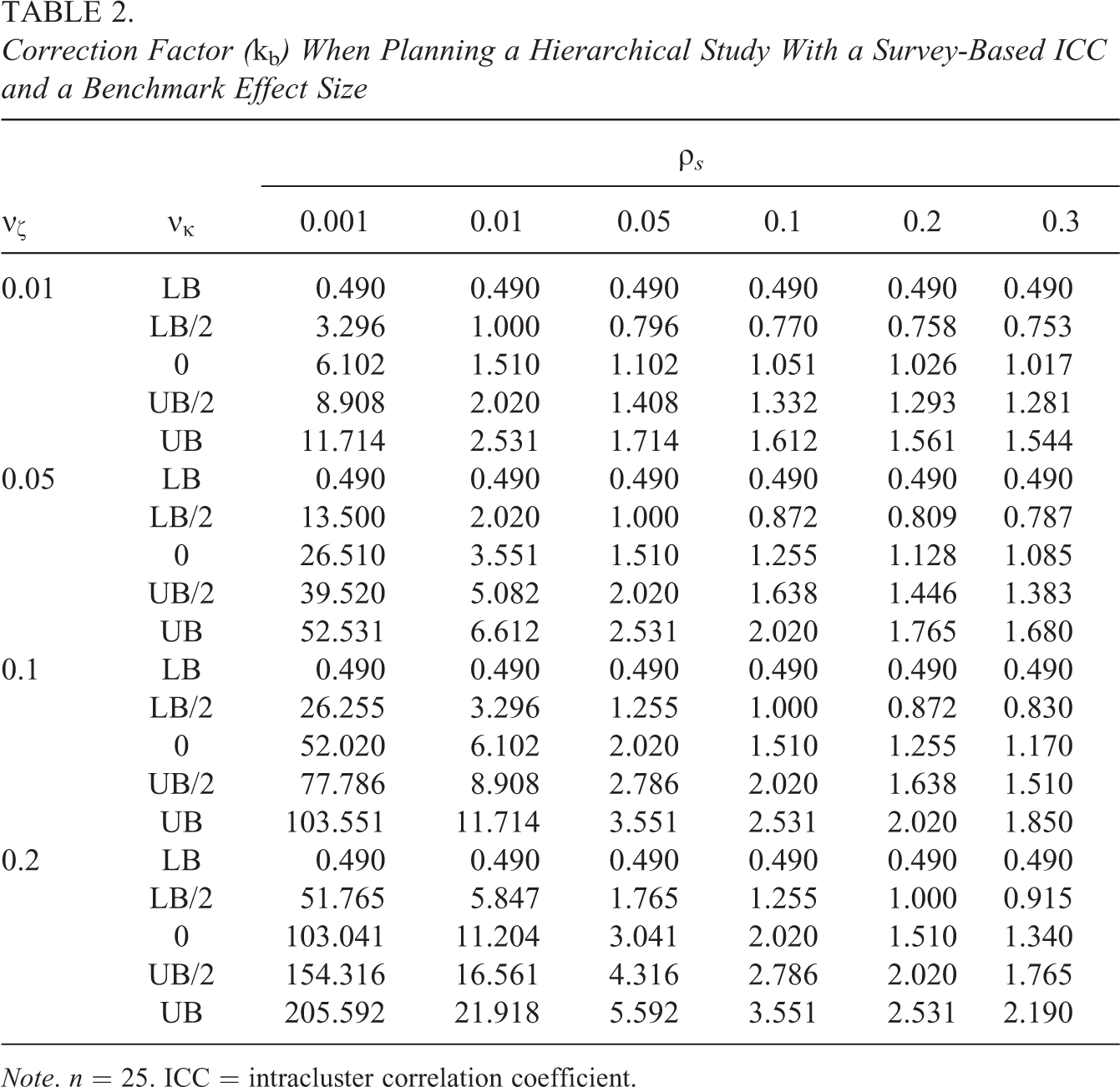
Note. n = 25. ICC = intracluster correlation coefficient.

Since very little is known empirically about likely values of ν_κ, values to use for illustration were chosen to cover the entire logical range of possible values. Equation A17 shows that $| ν_{κ} | \leq (ν_{ζ} + ρ_{S}) / 2$ . Therefore, Tables 1 and 2 illustrate values of k_H and k_b at five equally spaced values of ν_κ. Define $LB = - (ν_{ζ} + ρ_{S}) / 2$ and $UB = (ν_{ζ} + ρ_{S}) / 2$ . The values of ν_κ utilized in the table are $LB, \frac{LB}{2}, 0, \frac{UB}{2}, UB$ . While all five values are used to illustrate the range of possibilities, it seems unlikely that ν_κ would attain its lower or upper bound. Thus, discussion is focused on results when ν_κ equals LB/2, 0, or UB/2.

While Tables 1 and 2 reveal some extremely large adjustment factors, these numbers occur exclusively in conjunction with low values of the ICC (0.001 and 0.01). In these cases, the required school-level sample size to achieve an acceptable power level will be relatively low. So the impact of treatment effect heterogeneity on the required sample size may not be as large as these adjustment factors would seem to imply. When the ICC is at least 0.05, the adjustment factor ranges between 0.49 and 5.59 across all design scenarios examined in both tables. Examining only the middle three values of the covariance parameter (ignoring the extreme bounds), the adjustment factor is between 0.76 and 4.3.

Unfortunately, but not unexpectedly, the degree of the adjustment factor depends strongly on the ν_κ parameter about which there is currently little empirical evidence. The adjustment factor could be either substantially less than 1 (indicating a smaller sample size requirement than would be computed with unadjusted parameters) or many times more than 1 (indicating a larger sample size requirement than would be computed with unadjusted parameters).

It is perhaps reasonable to focus attention on results for a ρ_S value of 0.2 and a ν_ζ value of 0.05, as 0.2 would be considered a reasonable ICC for studies of academic achievement and 0.05 is a typical (somewhat low) estimate of ν_ζ based on both the rules of Raudenbush and Liu (2000) and existing empirical estimates. Specification of a relatively low value of ν_ζ and a relatively high value of ρ_S will tend to minimize the extent of the necessary adjustment to ρ_S. I continue to focus attention on the middle three values of the ν_κ parameter. With these restrictions, the correct ICC to use for the power analysis can be anywhere from 15% lower than ρ_S to 30% larger than ρ_S (if the denominator of the effect size is correct) or from 20% lower than ρ_S to 40% larger than ρ_S (if δ_bench is used).

Impact of Adjustment on Required School-Level Sample Size for Hierarchical Designs

The table and figure presented in this subsection explore the impact of the adjustment factor on the school-level sample size required to conduct a hierarchical trial. Results in this subsection assume that a researcher will conduct a power analysis to determine the necessary school-level sample size to attain statistical power of 0.80 to reject the null hypothesis of no average treatment effect (assuming a two-sided hypothesis test and 0.05 Type I error rate). In the interest of being concise, results are presented only for the case where ρ_S and δ_bench are used to plan the study (so that k_b is the appropriate adjustment factor). Examination of Equations 26 and 29 and Tables 1 and 2 reveals that k_b and k_H are generally reasonably close for a particular design scenario and that changes in design parameters have similar effects on k_b and k_H. So the results for k_b are reasonable approximations to what would be expected for k_H.

Table 3 uses the same values of ν_ζ, ν_κ, and ρ_S used in Tables 1 and 2. It is assumed that δ_bench = 0.25 and n = 25. For each configuration of the parameters, the required school-level sample size using the results from this article is compared to the sample size that would be computed if heterogeneity was ignored. Fractional sample sizes are rounded up to the next highest whole number.

Table 3.

Minimum School-Level Sample Size to Achieve 0.80 Power When Planning a Hierarchical Study With a Survey-Based ICC and a Benchmark Effect Size

		ρ _s
		0.001	0.01	0.05	0.1	0.2	0.3
Not adjusted		13	18	37	62	111	160
ν_ζ	ν_κ
0.01	LB	13	15	25	37	61	85
	LB/2	14	18	32	50	87	124
	0	16	20	40	64	113	163
	UB/2	17	23	47	78	140	202
	UB	18	25	55	92	166	241
0.05	LB	13	15	25	37	61	85
	LB/2	19	23	37	55	92	129
	0	26	30	50	74	124	173
	UB/2	32	38	62	93	155	217
	UB	38	45	75	112	186	261
0.1	LB	13	15	25	37	61	85
	LB/2	26	29	43	62	98	135
	0	38	43	62	87	136	185
	UB/2	51	56	81	112	174	236
	UB	64	70	100	137	211	286
0.2	LB	13	15	25	37	61	85
	LB/2	38	41	56	74	111	148
	0	63	68	87	112	161	210
	UB/2	88	94	119	150	211	273
	UB	114	120	150	187	262	336

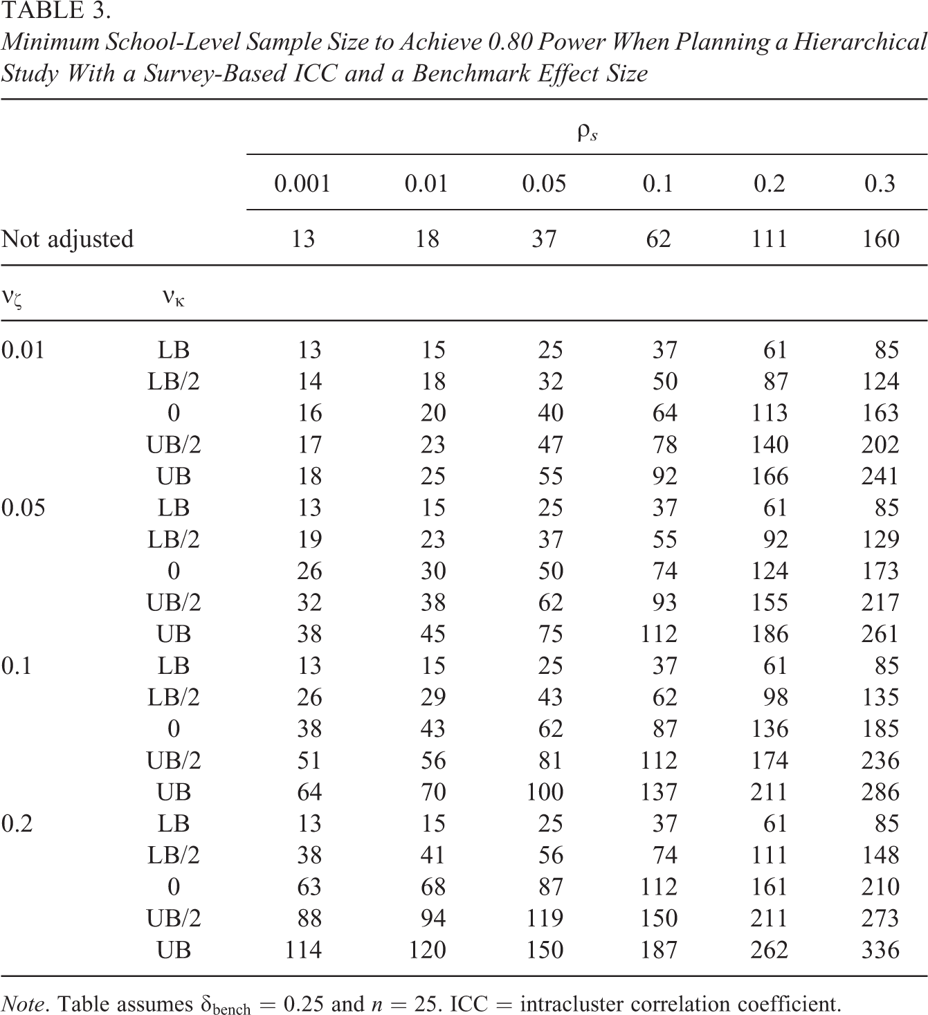
Note. Table assumes δ_bench = 0.25 and n = 25. ICC = intracluster correlation coefficient.

Table 3 illustrates that adjustments for heterogeneity can have a large impact on the school-level sample size necessary to conduct a hierarchical trial with 0.80 power. Unless both the ICC and the heterogeneity parameter are very small, there are large differences between the adjusted and unadjusted sample sizes. For instance, consider the case of a ν_ζ value of 0.01 and a ρ_S value of 0.1. When heterogeneity is ignored, the power analysis indicates the need for 62 schools in the study (assuming δ_bench = 0.25 and n = 25). If one assumes a moderate negative correlation between treatment effects and school-specific control group means (ν_κ = LB/2), one would need 12 less schools for 0.80 power. If one assumes no correlation between treatment effects and school-specific control group means (ν_κ = 0), one would need two more schools for 0.80 power. If one assumes a moderate positive correlation between treatment effects and school-specific control group means (τ_δ,cov = UB/2), one would need 16 more schools for 0.80 power.

Figure 1 plots the required sample size to achieve 0.80 power against the assumed benchmark effect size. The range of benchmark effect sizes considered is from 0.2 to 0.4, which encompasses the usual range of effect sizes used in educational studies. Both panels assume ρ_s = 0.15 and ν_ζ = 0.05. The solid line represents the (incorrect) sample size that would be computed if the survey-based ICC and effect size values were to be used without correction. The broken lines represent the correct sample sizes incorporating various assumptions about treatment effect heterogeneity. The value of n is set to a low value (n = 5) in the left panel and a high value (n = 100) in the right panel.

Figure 1.

School-level sample size as a function of assumed benchmark effect size when ρ _s = 0.15, ν_ζ = 0.05, n = 5 (left panel), and n = 100 (right panel).

The figure illustrates the extent to which school-level sample size is over- or underestimated, as the effect size varies. Note that the ratio of the correct sample size to the incorrect sample size is virtually constant as a function of the effect size. When n = 5, using uncorrected parameters overestimates the sample size by about 11% when there is a moderate negative correlation (ν_κ = −.05) between treatment effects and control group means, underestimates the sample size by about 10% when there is no correlation between treatment effects and control group means, and underestimates the sample size by about 24% when there is a moderate positive correlation (ν_κ = 0.05) between treatment effects and control group means. When n = 100, using uncorrected parameters overestimates the sample size by about 19% when there is a moderate negative correlation (ν_κ = −0.05) between treatment effects and control group means, underestimates the sample size by about 14% when there is no correlation between treatment effects and control group means, and underestimates the sample size by about 32% when there is a moderate positive correlation (ν_κ = 0.05) between treatment effects and control group means.

Using the Results in This Article to Plan a Multisite Study

As noted above, if a multisite study is planned using estimates of ρ_S, δ_bench and ν_ζ, then no adjustments to the parameters are necessary. However, if a multisite study is planned using a prior effect size estimate from a hierarchical study (δ_prev,H), this estimate will need to be adjusted by the factor k_M defined in Equation 33 to result in a correct power analysis. In this case, the adjustment is necessary to remove the impact of heterogeneity from the variance component in the denominator of the effect size estimate. Equation 33 makes clear that unless the covariance between treatment effects and school-specific control group means is strong and negative, the adjustment will tend to increase the effect size used in the power analysis and so will result in less schools needed to achieve a given level of power.

Since the form of the equation for k_M is rather simple, computations illustrating values of k_M are not presented. Instead, Table 4 presents the necessary school-level sample size to attain statistical power of 0.80 to reject the null hypothesis of no average treatment effect (assuming a two-sided hypothesis test and 0.05 Type I error rate). The table assumes δ_prev,H = 0.25 and n = 26 (to ensure a balanced design). The school-level sample size computed using the adjustment factor is compared to the sample size that would be computed if the effect size was not adjusted to account for heterogeneity. The values of ν_ζ and ν_κ used in the table are the same used for previous tables. Only values of ρ_s of 0.01 or greater are used, since there is little value in multisite designs when the ICC is very low.

Table 4.

Minimum School-Level Sample Size to Achieve 0.80 Power When Planning a Multisite Study With a Survey-Based ICC and an Effect Size Estimate From a Previous Hierarchical Study

		ρ_s
ν_ζ	ν_κ	.01	0.05	0.1	0.2	0.3
0.01	Not adjusted	13	13	13	12	11
	LB	13	13	13	13	12
	LB/2	13	13	13	12	11
	0	13	13	12	12	11
	UB/2	13	13	12	11	10
	UB	13	13	12	11	10
0.05	Not adjusted	18	18	17	17	16
	LB	18	18	18	18	18
	LB/2	18	18	18	17	16
	0	18	18	17	16	15
	UB/2	18	17	17	15	14
	UB	18	17	16	15	13
0.1	Not adjusted	25	24	24	23	22
	LB	25	25	25	25	25
	LB/2	24	24	24	23	23
	0	24	23	23	22	21
	UB/2	23	22	22	21	19
	UB	23	22	21	19	18
0.2	Not adjusted	37	37	36	35	34
	LB	37	38	38	39	40
	LB/2	36	36	35	35	35
	0	34	34	33	32	31
	UB/2	33	32	31	30	29
	UB	31	30	30	28	26

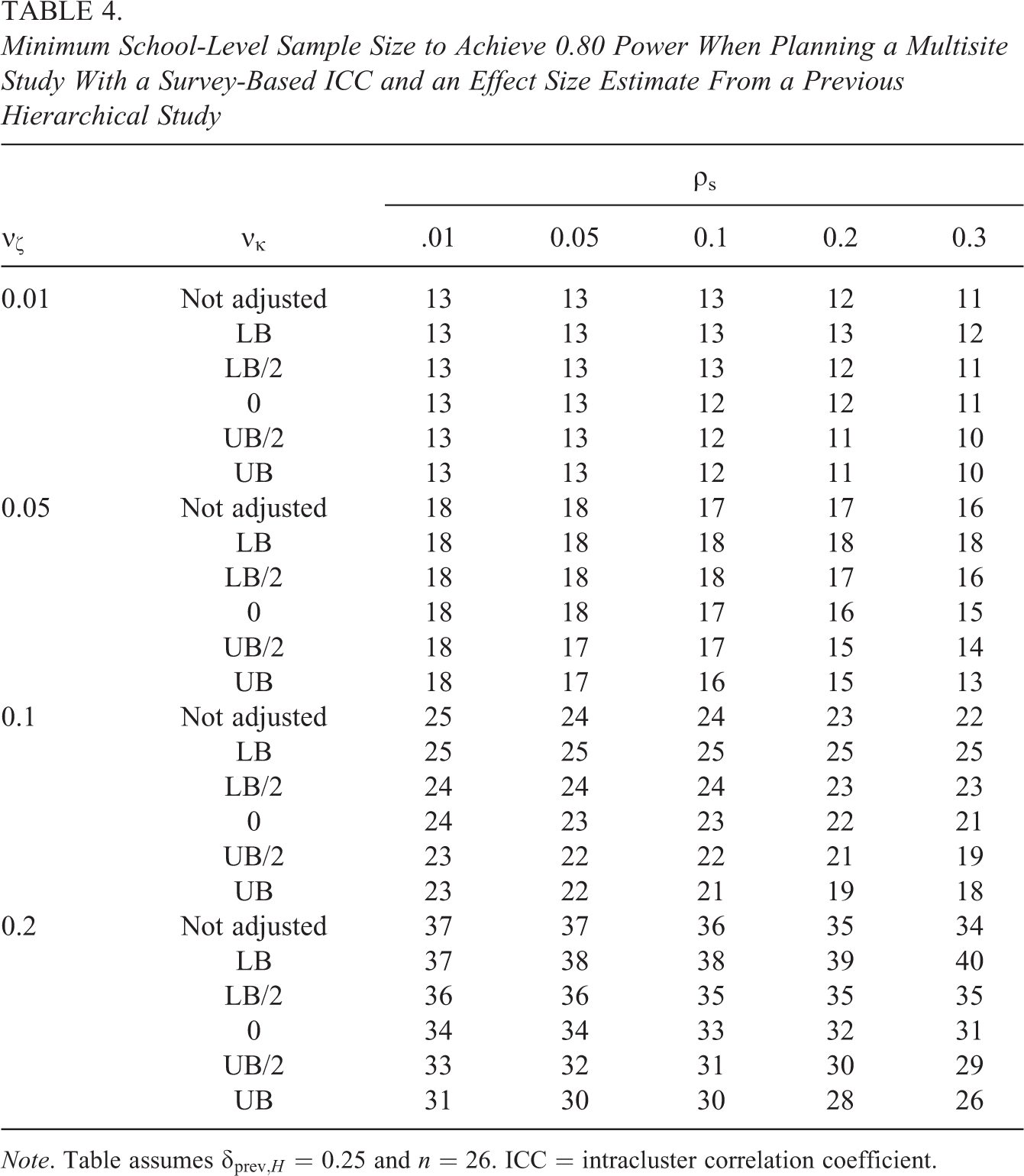
Note. Table assumes δ_prev,H = 0.25 and n = 26. ICC = intracluster correlation coefficient.

Results presented in Table 4 show that adjusting to remove heterogeneity from the denominator of an effect size estimate when planning a multisite design makes little difference when the goal is to compute the school-level sample size necessary to achieve 0.80 power. This is in stark contrast to hierarchical designs where adjustments to account for heterogeneity make a large difference in the necessary school-level sample size.

Example Power Analysis

In order to further illustrate the appropriate use of the results in this article, this section provides an example of a design scenario that requires a power analysis. The example assumes that the sample for the study will involve students nested within schools. The required school-level sample size is computed, given assumptions about other relevant design parameters. School-level sample size is computed both with and without the adjustments recommended in this article.

Example

Researchers are studying an intervention designed to improve math skills in second graders. Their study will be conducted among low achieving rural schools in the Midwest. Entering the relevant specifications into the online variance almanac (Hedges & Hedberg, 2016), they obtain the value ρ_S = 0.094. There is no previous research on this intervention, but they believe it is reasonable to assume that the intervention will increase student annual growth on a standardized math assessment by 25%. Due to the nature of the population being studied, the researchers assume most students will be below the 25th percentile on nationally normed math tests. Referencing table 3 of Scammacca et al. (2015), they determine that average annual growth in second grade across four standardized math tests is 1.07. Therefore, they assume an effect size of the intervention of δ_bench = 1.07 × 0.25 = 0.2675. Due to the rural population being studied, the researchers believe that only 20 students per school will be available for the study, so that 2n = 20.

Power Analysis for a Hierarchical Design

Assume initially that the researchers plan to conduct a school randomized design, perhaps due to concerns about contamination (Rhoads, 2011). A standard power analysis would enter ρ_S, δ_bench, and 2n into a software program such as OD Plus and then compute the school-level sample size necessary to achieve 0.80 power with a Type I error rate of 0.05. Performing this calculation in OD Plus results in a required school-level sample size of m = 64.

Now assume that the researchers desire to appropriately account for treatment effect heterogeneity in their power analysis. Since the study will be conducted in a variety of different rural communities, the researchers decide to assume a moderate to high level of treatment effect heterogeneity, with ν_ζ = 0.08. Assume there is no existing empirical information about the covariance between school average treatment effects and school average values of the outcome in the control group. However, the researchers believe this covariance will be small and positive. Therefore, they decide to compute the required school-level sample size using two different assumptions: (1) assuming a 0 covariance and (2) assuming covariance equal to one half of the logical upper bound.

To compute the necessary correction factor from Equation 29, it is first necessary to compute $ν_{T} = ν_{ζ} + 2 \times ν_{κ}$ . When there is a 0 covariance, ν_T = ν_ζ and the necessary correction factor is 1.45. To compute the necessary correction factor under the second assumption, first divide Equation A16 by 2(τ_C + σ²) in order to show that the upper bound for ν_κ is $ν_{κ} \leq (ρ_{S} + ν_{ζ}) / 2$ . Substituting 0.094 for ρ_S and 0.08 for ν_ζ gives the upper bound for ν_κ of 0.087, so that one half of this bound is 0.0435. Substituting this number into the definition of ν_T gives the result $ν_{T} = ν_{ζ} + 2 \times ν_{κ} = .167$ . The correction factor is then computed from Equation 29 as 1.94.

The researchers would now enter OD Plus, using 0.094 × 1.45 = 0.136 as the ICC under the first scenario and 0.094 × 1.94 = 0.182 under the second scenario. The resulting school-level sample sizes would be m = 80 and m = 100, respectively.

Power Analysis for a Multisite Design

A required sample size of 80 to 100 schools may seem unrealistically large for many educational studies. In such cases, it could be useful for researchers to consider a design that randomly assigns within schools. Rhoads (2011) has shown that, even in the presence of substantial contamination, such a design can provide more statistical power than a hierarchical design. Hence, we now assume that contamination will decrease the observable effect size by about 20%, so that the effect size to use in the power analysis is 0.8 × 0.2675 = 0.214. To compute power for a multisite design in OD Plus, it is necessary to specify a parameter $ν_{w} = \frac{ζ}{σ_{}^{2}} = \frac{ν_{ζ}}{1 - ρ_{s}}$ . In this case, its value is 0.08/0.906 = 0.088. Given these parameters, OD Plus computes the necessary school-level sample size as m = 52. As noted in the article, this power analysis is correct without further adjustments to parameters.

Conclusion

This article has illustrated the impact of heterogeneity in treatment effects across schools on the planning of educational experiments where students are nested within schools. Both hierarchical and multisite designs have been considered. A potential outcomes approach was used to equate the parameters that are necessary to compute power for multisite and hierarchical designs with parameters defined in terms of potential outcomes. This approach allows for equating the parameters necessary to compute power in hierarchical designs with the parameters necessary to compute power in multisite designs and vice versa.

One benefit of this equating is that it makes possible coherent comparisons between power computations for hierarchical and multisite designs. Using results in this article, researchers can obtain an accurate idea of how the sample size requirement of a multisite study would compare to the sample size requirement of a hierarchical study, making the same assumptions about relevant design parameters and conducted on the same population of schools.

Results presented earlier illustrate that a power analysis for a multisite study can be performed accurately using benchmark effect sizes and survey-based ICCs without the need for adjustments. However, benchmark effects sizes and/or survey-based ICCs will need to be adjusted to account for treatment effect heterogeneity in order to produce an accurate power analysis for a hierarchical study. This article has derived the necessary adjustments. The adjustments can be quite consequential, even when heterogeneity in treatment effects is not particularly large.

The extent of the necessary adjustment for heterogeneity depends crucially on the covariance between treatment effects and control group means. While this parameter can be estimated from multisite studies, there has been little to no effort to report values of this parameter in the existing literature. This lack of information is an important obstacle to effectively conducting a power analysis for a hierarchical study of an educational intervention.

Fortunately, it is possible that help is on the way. Recent years have seen a number of papers published on the topic of heterogeneity of treatment effects across sites (e.g., Chaney, 2016; Raudenbush, Reardon, & Nomi, 2012, and commentary; Raudenbush & Bloom, 2015; Weiss, Bloom, & Brock, 2014). Raudenbush and Bloom (2015) describe a procedure for the direct estimation of the covariation between treatment effects and school-specific control group means. It is hoped that the recent methodological work on the topic will lead to a corresponding increase in the reporting of this crucial design parameter.

In the meantime, there are some steps that researchers can take to try to improve the accuracy of their power analyses by accounting for treatment effect heterogeneity. The ideal approach would be to conduct a pilot study that would allow for the estimation of the covariance between school-level control group means and school-level treatment effects using the method outlined in Raudenbush and Bloom (2015).

If empirical evidence cannot be obtained, it is still possible that a researcher’s knowledge of the intervention will allow an educated guess regarding the covariance between treatment effects and control group means. For instance, one might hypothesize that high functioning schools will be able to leverage their superior organizational capacity to take better advantage of educational innovations relative to lower functioning schools. This would argue for assuming a positive covariance between treatment effects and control group means. On the other hand, the goal of some educational interventions is to remediate deficiencies. In this case, a negative covariance between treatment effects and control group means should be anticipated.

Another approach is to conduct a sensitivity analysis to determine how the required school-level sample size changes as a function of assumptions about the covariance of treatment effects with control group means. Since the required school-level sample size for hierarchical designs increases as this covariance increases, the cautious researcher will want to err on the side of assuming the covariance to be large and positive. Of course, budgetary constraints will preclude taking this advice too far.

The lack of good empirical estimates of relevant parameters leaves researchers with less than desirable options. However, ignoring treatment effect heterogeneity involves an implicit assumption that this heterogeneity is zero. The current article shows that this can lead to large errors in the estimated sample size from a power analysis. Even relatively uneducated guesses about important design parameters are likely to be preferable to making the assumption of zero heterogeneity.

Footnotes

Declaration of Conflicting Interests

The author(s) declared no potential conflicts of interest with respect to the research, authorship, and/or publication of this article.

Funding

The author(s) received no financial support for the research, authorship, and/or publication of this article.

References

Angrist

J. D.

(2004). American education research changes tack. Oxford Review of Economic Policy, 20, 198–212.

Angrist

J. D.

Imbens

G. W.

Rubin

D. B.

(1996). Identification of causal effects using instrumental variables. Journal of the American Statistical Association, 91, 444–455.

Bloom

H. S.

Hill

Rebeck Black

Lipsey

(2008). Performance trajectories and performance gaps as achievement effect-size benchmarks for educational interventions. Journal of Research on Educational Effectiveness, 1, 289–328.

Bloom

H. S.

Weiland

(2015). Quantifying variation in head start effects on children’s cognitive and socio-emotional skills using data from the national head start impact study (MDRC Working Paper on Research Methodology). New York, NY: MDRC.

Borenstein

Hedges

L. V.

Rothstein

(2012). CRT power. Teaneck, NJ: Biostat.

Brandon

P. R.

Harrison

G. M.

Lawton

B. E.

(2013). SAS Code for calculating intraclass correlation coefficients and effect size benchmarks for site randomized education experiments. American Journal of Evaluation, 34, 85–90.

Casella

Berger

(2002). Statistical inference (2nd ed.). Pacific Grove, CA: Duxbury.

Chaney

(2016). Reconsidering findings of “no effects” in randomized controlled trials: Modeling differences in treatment impacts. American Journal of Evaluation, 37, 45–62.

Cohen

(1988). Statistical power analysis for the behavioral sciences (2nd ed.). Hillsdale, NJ: Lawrence Erlbaum.

10.

Constas

(2007). Reshaping the methodological identity of education research: Early signs of the impact of federal policy. Evaluation Review, 31, 391–400.

11.

Hedges

L. V.

Hedberg

E. C.

(2007a). Intraclass correlation values for planning group-randomized trials in education. Educational Evaluation and Policy Analysis, 29, 60–87.

12.

Hedges

L. V.

Hedberg

E. C.

(2007b). Intraclass correlations for planning group randomized experiments in rural education. Journal of Research in Rural Education, 22, 1–15.

13.

Hedges

L. V.

Hedberg

E. C.

(2016). Power calculation using the online variance almanac (Web VA): A user’s guide. Retrieved July 2016, from https://arc.uchicago.edu/sites/default/files/VA%20User%20Guide.pdf

14.

Hedges

L. V.

Rhoads

(2009). Statistical power analysis in education research (NCSER 2010-3006). Washington, DC: National Center for Special Education Research, Institute of Education Sciences, U.S. Department of Education.

15.

Holland

(1986). Statistics and causal inference. Journal of the American Statistical Association, 81, 945–960.

16.

Jacob

Zhu

Bloom

(2010). New empirical evidence for the design of group randomized trials in education. Journal of Research on Educational Effectiveness, 3, 157–198.

17.

Kim

Olson

C. B.

Scarcella

Kramer

Pearson

van Dyk

… Land

(2011). A randomized experiment of a cognitive strategies approach to test-based analytical writing for mainstreamed Latino English language learners in grades 6 to 12. Journal of Research on Educational Effectiveness, 4, 231–263.

18.

Kish

(1965). Survey sampling. New York, NY: Wiley.

19.

Konstantopoulos

(2008). The power of the test for treatment effects in three-level block randomized designs. Journal of Research on Educational Effectiveness, 1, 265–288.

20.

Kosko

Miyazaki

(2012). The effect of student discussion frequency on fifth-grade students’ mathematics achievement in U.S. schools. The Journal of Experimental Education, 80, 173–195.

21.

National Center for Education Research. (2015). FY 2016 request for applications. Retrieved from http://ies.ed.gov/funding/ncer_progs.asp

22.

Raudenbush

S. W.

(1997). Statistical analysis and optimal design for cluster randomization trials. Psychological Methods, 2, 173–185.

23.

Raudenbush

S. W.

Bloom

H. S.

(2015). Learning about and from a distribution of program impacts using multisite trials. American Journal of Evaluation, 36, 475–499.

24.

Raudenbush

S. W.

Liu

(2000). Statistical analysis and optimal design for multisite randomized trials. Psychological Methods, 5, 199–213.

25.

Raudenbush

S. W.

Reardon

Nomi

(2012). Statistical analysis for multisite trials using instrumental variables with random coefficients. Journal of Research on Educational Effectiveness, 5, 303–332.

26.

Raudenbush

S. W.

Spybrook

Congdon

Liu

Martinez

Bloom

Hill

(2011). Optimal design plus empirical evidence (Version 3.0). Retrieved from http://hlmsoft.net/od/od-manual-20111016-v300.pdf

27.

Rhoads

(2011). The implications of contamination for experimental design in education research. Journal of Educational and Behavioral Statistics, 36, 76–104.

28.

Rosenbaum

P. R.

Rubin

D. B.

(1983). The central role of the propensity score in observational studies for causal effects. Biometrika, 70, 41–55.

29.

Rubin

D. B.

(1974). Estimating causal effects of treatments in randomized and nonrandomized studies. Journal of Educational Psychology, 66, 688–701.

30.

Scammacca

Fall

A. M.

Roberts

(2015). Benchmarks for expected annual academic growth for students in the bottom quartile of the normative distribution. Journal of Research on Educational Effectiveness, 8, 366–379.

31.

Schochet

(2008). Statistical power for random assignment evaluations of education programs. Journal of Educational and Behavioral Statistics, 33, 62–87.

32.

Spybrook

(2014). Introduction to special issue on design parameters for cluster randomized trials in education, Evaluation Review, 37, 435–444.

33.

Spybrook

Cullen

Lininger

(2011). An examination of the impact of changes in federal policy on the landscape of education research. Effective Education, 3, 83–88.

34.

Spybrook

Hedges

Borenstein

(2014). Understanding statistical power in cluster randomized trials: Challenges posted by differences in notation and terminology. Journal of Research on Educational Effectiveness, 7, 384–406.

35.

Weiss

Bloom

H. S.

Brock

(2014). A conceptual framework for studying the sources of variation in program effects. Journal of Policy Analysis and Management, 33, 778–808.

36.

Westine

Spybrook

Taylor

. (2013). An empirical investigation of variance design parameters for planning cluster-randomized trials of science achievement. Evaluation Review, 37, 490–519.

37.

Whitehurst

G. J.

(2004, 4 26). Making education evidence-based: Premises, principles, pragmatics, and politics (IPR Distinguished Public Policy Lecture Series, 2003-2004). Evanston, IL: Northwestern University, Institute for Policy Research.

38.

Nichols

(2010). New estimates of design parameters for clustered randomization studies: Findings from North Carolina and Florida (Calder Working Paper Number 43). Washington, DC: CALDER.

Supplementary Material

Please find the following supplemental material available below.

For Open Access articles published under a Creative Commons License, all supplemental material carries the same license as the article it is associated with.

For non-Open Access articles published, all supplemental material carries a non-exclusive license, and permission requests for re-use of supplemental material or any part of supplemental material shall be sent directly to the copyright owner as specified in the copyright notice associated with the article.

0.00 MB

0.17 MB

Coherent Power Analysis in Multilevel Studies Using Parameters From Surveys

Abstract

Keywords

Linear Mixed Models for the Analysis of Two-Level Multisite and Hierarchical Studies

The Model for the Hierarchical Design

The Model for the Multisite Design

Interpreting Parameters Using Potential Outcomes

Existing Empirical Work to Determine Design Parameters for Education Research

Empirical Estimates of ICCs for Designs With Students Nested Within Schools

Benchmark Effect Sizes for Educational Evaluations

Empirical Estimates of the Standardized Effect Size Variance

Adjusting Design Parameters to Account for the Effects of Heterogeneity

Adjustments When Planning a Hierarchical Trial

Using δprev,H

Using δbench

Using δprev,W

Adjustments When Planning a Multisite Trial

Using δbench

Using δprev,W

Using δprev,H

Illustrations Using the Above Results

Illustrative Values of Adjustment Factors for Hierarchical Designs

Impact of Adjustment on Required School-Level Sample Size for Hierarchical Designs

Using the Results in This Article to Plan a Multisite Study

Example Power Analysis

Example

Power Analysis for a Hierarchical Design

Power Analysis for a Multisite Design

Conclusion

Footnotes

Declaration of Conflicting Interests

Funding

References

Supplementary Material

Using δ_prev,H

Using δ_bench

Using δ_prev,W

Using δ_bench

Using δ_prev,W

Using δ_prev,H