Optimizing individual activity personal plans through local search

Abstract

Optimization through local search is known to be a powerful approach to confront complex optimization problems. In this article we tackle the problem of optimizing individual activity personal plans, that is, plans involving activities one person has to accomplish independently of others, taking into account complex constraints and preferences. Recently, this problem has been addressed adequately using an adaptation of the squeaky wheel optimization framework (SWO). In this article we demonstrate that further improvement can be achieved in the quality of the resulting plans, by coupling SWO with a post-optimization phase based on local search techniques. Particularly, we present a bundle of transformation methods to explore the neighborhood of the solution produced by SWO using either hill climbing or simulated annealing. Similar results can be obtained by employing local search only, starting from an empty plan, thus demonstrating the strength of the proposed local search techniques. We present several experiments that demonstrate an improvement on the utility of the produced plans, with respect to the solutions produced by SWO only, of more than 6% on average, which in particular cases exceeds 20%. Of course, this improvement comes at the cost of extra time.

Keywords

Local search personal activities scheduling

1. Introduction

Electronic calendar applications and personal digital assistants typically involve sets of fully specified and independent events. These events constitute a user’s schedule for a period of time. They are usually characterized by a fixed start time, a duration and, occasionally, a location where that particular event will take place. Furthermore, many systems support tasks. These are commitments potentially having a deadline to be met (e.g., writing an article or doing weekly shopping). Tasks are often kept separately, in task lists, and are not characterized by a specific start time. In some systems, as soon as a task is dropped into the calendar, it is automatically transformed into an event. The need to develop intelligent automated systems for calendar management has been identified by many researchers as an ambitious task for Artificial Intelligence [3,4,7,12,14–16].

In other work [18], a constraint optimization model for the problem of managing personal time is presented, treating events and tasks, referred as activities, in a uniform way. Each activity is characterized by a temporal domain, a duration profile, a set of possible alternative locations, preemptiveness (that is, possibility of being interrupted and resumed), utilization (that is, possibility of being performed concurrently with other activities), various preferences over its temporal domain and its duration profile, as well as constraints and preferences over the way parts of an interruptible activity are scheduled in time. The model also supports a variety of binary constraints and preferences, particularly ordering, proximity and implication relations. In the same work, a scheduler, based on the squeaky wheel optimization (SWO) framework and coupled with domain-dependent heuristics, is employed to automatically schedule a user’s individual activities. SWO is a powerful but incomplete search algorithm, so the solutions it produces are generally not optimal. This sub-optimality is more apparent in over-constrained, though practical problems, where SWO often produces schedules that a user can manually improve through simple transformations, such as scheduling an activity at a more preferred time point.

This last observation motivated us to improve upon SWO’s solution quality. Post-optimization modules developed for planners recently, that exploit a plan’s structure, have proven to be effective [5,6,11,13,19]. So, in this article we present local-search techniques that increase the quality of SWO’s plan output through post-optimization. In the particular setting, we devised and implemented a set of transformations of valid plans, such as shifting activities, changing their durations and locations, as well as merging or splitting parts of interruptible activities. Extensive experimental results have shown improvement over SWO’s output up to 20.38%. In addition, we explore the contribution of each particular transformation on improving a schedule. Finally, we demonstrate that similar results can be achieved by commencing local search from the empty plan, thus demonstrating the strength of the designed bundle of transformations. However, post-processing dominates pure local search in hard problems, when the available computation time is bounded.

Earlier stages of this work have been presented [1,2]. This article elaborates over previous work of the same authors in that (a) it advances the underlying stochastic local search algorithms by employing some form of stochastic backtracking during local search, as well as by relaxing the seed solution in over-constrained problems prior to local search; (b) it provides detailed experimental results, including evaluating the contribution of each individual transformation to the final output; (c) it illustrates the effectiveness of the proposed local search optimization algorithms through a realistic scenario; and (d) it discusses usability and transferability issues.

The rest of the article is structured as follows. First, we formulate the constraint optimization problem and illustrate the SWO-based approach. We also briefly discuss usability issues. Next, we present the local search transformations to explore the neighborhood during the post-optimization phase, using either hill-climbing or simulating annealing [8,10]. Subsequently, we present experimental results over a large set of problem instances, taken from previous work [18]. Furthermore, we demonstrate the strength of the local search techniques when applied to an empty plan. Then we evaluate the contribution of each particular transformation on the post-optimization process. We conclude our evaluation by applying the proposed methods to a realistic scenario. Finally, we discuss the results, before summarizing the article and identifying directions of future work.

2. Background

In this section we outline the problem formulation, as well as the SWO approach adopted in [18] to cope with the problem. Furthermore, we briefly discuss usability issues.

2.1. Problem formulation

Time is considered a non-negative integer, with zero denoting the current time. A set T of N activities, $T = {T_{1}, T_{2}, \dots, T_{N}}$ , is assumed. For each activity $T_{i} \in T$ , its minimum duration is denoted with $d_{i}^{min}$ and its maximum duration with $d_{i}^{max}$ . No activity can be accomplished with a scheduled duration less than $d_{i}^{min}$ . On the other hand, there is no point in allocating more than $d_{i}^{max}$ to $T_{i}$ . A greater duration in the range $[d_{i}^{min}, d_{i}^{max}]$ results in greater utility for the user.

The decision variable $p_{i}$ denotes the number of parts in which $T_{i}$ has been split, with $p_{i} ⩾ 1$ when $T_{i}$ has been scheduled. $T_{i j}$ denotes the jth part of $T_{i}$ , $1 ⩽ j ⩽ p_{i}$ . Non-interruptible activities are scheduled as one part, that is, $p_{i} = 1$ , $\begin{matrix} (C1) & \forall T_{i} : p_{i} = \{\begin{matrix} 0 & if T_{i} is not scheduled, \\ 1 & if T_{i} is not interruptible, \\ ⩾ 1 & if T_{i} is interruptible . \end{matrix} \end{matrix}$ For each $T_{i j}$ , the decision variables $t_{i j}$ and $d_{i j}$ denote its start time and duration. The sum of all $d_{i j}$ , for a given i, is denoted with $d_{i}$ , $\begin{matrix} (C2) & \forall T_{i} : \sum_{j = 1}^{p_{i}} d_{i j} = d_{i}, \end{matrix}$ which must be at least $d_{i}^{min}$ , or 0 if $T_{i}$ is not scheduled, $\begin{matrix} (C3) & \forall T_{i} : d_{i}^{min} ⩽ d_{i} or d_{i} = 0 . \end{matrix}$

For each $T_{i}$ we define the minimum and maximum possible part duration, ${smin}_{i}$ and ${smax}_{i}$ , $\begin{matrix} (C4) & \forall T_{i j} : {smin}_{i} ⩽ d_{i j} ⩽ {smax}_{i} or d_{i j} = 0, \end{matrix}$ as well as the minimum and maximum allowed temporal distances between every pair of parts, ${dmin}_{i}$ , $\begin{matrix} (C5) & \begin{matrix} \forall T_{i j}, T_{i k}, j \neq k, d_{i j} > 0, d_{i k} > 0 : \\ t_{i j} + d_{i j} + {dmin}_{i} ⩽ t_{i k} \lor t_{i k} + d_{i k} + {dmin}_{i} \\ ⩽ t_{i j}, \end{matrix} \end{matrix}$ and ${dmax}_{i}$ , $\begin{matrix} (C6) & \begin{matrix} \forall T_{i j}, T_{i k}, j \neq k, d_{i j} > 0, d_{i k} > 0 : \\ t_{i j} + {dmax}_{i} ⩾ t_{i k} + d_{i k} \land t_{i k} + {dmax}_{i} \\ ⩾ t_{i j} + d_{i j} . \end{matrix} \end{matrix}$

For each $T_{i}$ , its temporal domain is defined as a set of temporal intervals $D_{i} = [a_{i 1}, b_{i 1}) \cup [a_{i 2}, b_{i 2}) \cup \dots \cup [a_{i, F_{i}}, b_{i, F_{i}})$ , where $F_{i}$ is the number of these intervals. All parts of $T_{i}$ must be scheduled within $D_{i}$ , $\begin{matrix} (C7) & \begin{matrix} \forall T_{i j}, d_{i j} > 0 : \\ \exists k, 1 ⩽ k ⩽ F_{i}, a_{i k} ⩽ t_{i j} ⩽ b_{i k} - d_{i j} . \end{matrix} \end{matrix}$

A set of M locations, $Loc = {L_{1}, L_{2}, \dots, L_{M}}$ , as well as a two-dimensional, not necessarily symmetric, matrix $Dist$ that holds the temporal distances between locations are given. To each activity $T_{i}$ a set of possible locations ${Loc}_{i} \subseteq Loc$ , where its parts can be scheduled, is assigned. The decision variable $l_{i j} \in {Loc}_{i}$ , $\begin{matrix} (C8) & \forall T_{i j} : l_{i j} \in {Loc}_{i}, \end{matrix}$ denotes the particular location where $T_{i j}$ is scheduled. Every pair of distinct activity parts $T_{i j}$ and $T_{m n}$ scheduled in different locations must have a minimum temporal distance of $Dist (l_{i j}, l_{m n})$ or $Dist (l_{m n}, l_{i j})$ , depending on which part is scheduled earlier in time, $\begin{matrix} (C9) & \begin{matrix} \forall T_{i j}, T_{m n}, T_{i j} \neq T_{m n}, d_{i j} > 0, d_{m n} > 0 : \\ (Dist (l_{i j}, l_{m n}) > 0 \lor Dist (l_{m n}, l_{i j}) > 0) \\ ⟹ t_{i j} + d_{i j} + Dist (l_{i j}, l_{m n}) \\ ⩽ t_{m n} \lor t_{m n} + d_{m n} + Dist (l_{m n}, l_{i j}) \\ ⩽ t_{i j} . \end{matrix} \end{matrix}$

Activities may overlap in time. This is supported through the introduction of utilization, which measures the degree an activity absorbs the attention of the person performing it. Particularly, each $T_{i}$ is characterized by a utilization value, ${utilization}_{i}$ , taking values between 0 and 1. At any time point, the set of scheduled activities should have compatible locations (that is, locations with no temporal distance to each other) and the sum of their utilization values should not exceed the one unit, $\begin{matrix} (C10) & \forall t : \sum_{\begin{array}{c} T_{i j} \\ t_{i j} ⩽ t < t_{i j} + d_{i j} \end{array}} {utilization}_{i} ⩽ 1 . \end{matrix}$

The model supports four types of binary constraints: Ordering constraints, minimum and maximum proximity constraints and implication constraints. An ordering constraint between two activities $T_{i}$ and $T_{j}$ , denoted with $T_{i} < T_{j}$ , implies that no part of $T_{j}$ can start its execution before all parts of $T_{i}$ have finished, $\begin{matrix} (C11) & \begin{matrix} \forall T_{i}, T_{j}, d_{i} > 0, d_{j} > 0 : T_{i} < T_{j} \\ ⟹ \forall T_{i k}, T_{j l}, d_{i k} > 0, d_{j l} > 0 : \\ t_{i k} + d_{i k} ⩽ t_{j l} . \end{matrix} \end{matrix}$ A minimum (maximum) distance binary constraint between activities $T_{i}$ and $T_{j}$ implies every two parts, one of $T_{i}$ and another of $T_{j}$ , must have a given minimum (maximum) temporal distance, $\begin{array}{l} (C12) & \begin{matrix} \forall T_{i k}, T_{j l}, d_{i k} > 0, d_{j l} > 0, {dmin}_{i j} > 0 : \\ t_{i k} + d_{i k} + {dmin}_{i j} ⩽ t_{j l} \lor t_{j l} + d_{j l} + {dmin}_{i j} \\ ⩽ t_{i k}, \end{matrix} \\ (C13) & \begin{matrix} \forall T_{i k}, T_{j l}, d_{i k} > 0, d_{j l} > 0, {dmax}_{i j} < \infty : \\ t_{i k} + {dmax}_{i j} ⩾ t_{j l} + d_{j l} \land t_{j l} + {dmax}_{i j} \\ ⩾ t_{i k} + d_{i k} . \end{matrix} \end{array}$ Finally, an implication constraint of the form $T_{i} \Rightarrow T_{j}$ implies that in order to include $T_{i}$ in the plan, $T_{j}$ should be included as well, $\begin{array}{l} (C14) & \begin{matrix} \forall T_{i}, T_{j} : T_{i} ⟹ T_{j} \\ ⟺ (d_{i} > 0 ⟹ d_{j} > 0) . \end{matrix} \end{array}$

Alternative schedules may differ in their total utility, which is computed as the sum of the value accumulated from a variety of utility sources. The main source of utility concerns the inclusion of each particular activity $T_{i}$ in the schedule and is denoted with $U_{i} (d_{i})$ , taking its minimum value when $d_{i} = d_{i}^{min}$ and its maximum value when $d_{i} = d_{i}^{max}$ . A linear definition for $U_{i} (d_{i})$ is the following: $\begin{matrix} (1) & U_{i} (d_{i}) = \{\begin{matrix} 0 if d_{i} < d_{i}^{min}, \\ u_{i}^{low} + \frac{(d_{i} - d_{i}^{min})}{(d_{i}^{max} - d_{i}^{min})} (u_{i}^{high} - u_{i}^{low}) \\ if d_{i}^{min} ⩽ d_{i} ⩽ d_{i}^{max}, \\ u_{i}^{high} if d_{i} > d_{i}^{max}, \end{matrix} \end{matrix}$ where $u_{i}^{low}$ and $u_{i}^{high}$ are constants with $0 ⩽ u_{i}^{low} ⩽ u_{i}^{high}$ .

The way $T_{i}$ is scheduled by a schedule $π_{i}$ within its temporal domain constitutes another source of utility, $U_{i}^{time} (π_{i})$ , which is defined as: $\begin{matrix} (2) & U_{i}^{time} (π_{i}) = \frac{\sum_{j = 1}^{p_{i}} \sum_{t = t_{i j}}^{t_{i j} + d_{i j} - 1} u_{i}^{time} (t)}{d_{i}}, \end{matrix}$ where $u_{i}^{time} (t)$ denotes the utility accumulated by scheduling one unit of time of $T_{i}$ at t. Particularly, let t be a time slot in $T_{i}$ ’s kth interval $[a_{i k}, b_{i k})$ , that is, $a_{i k} ⩽ t < b_{i k}$ , $1 ⩽ k ⩽ F_{i}$ . Furthermore, we assume that for the arbitrary kth interval of $D_{i}$ , we are given two bound values, $u_{i k}^{low}$ and $u_{i k}^{high}$ . Then, $u_{i}^{time} (t)$ can be defined as: $\begin{matrix} (3) & u_{i}^{time} (t) = \{\begin{matrix} 0 if t < a_{i k} or t ⩾ b_{i k} for every k, \\ u_{i k}^{low} + (t - a_{i k}) \frac{u_{i k}^{high} - u_{i k}^{low}}{b_{i k} - a_{i k} - 1} \\ if t ⩾ a_{i k} and t < b_{i k} for some k . \end{matrix} \end{matrix}$

Any form of hard constraint can also be considered a soft constraint that might contribute utility. Partial satisfaction of ordering and proximity soft constraints is allowed. For example, minimum and maximum distance constraints between the parts of an interruptible activity contribute $U_{i}^{dmin} (π_{i})$ and $U_{i}^{dmax} (π_{i})$ , respectively: $\begin{array}{rcl} U_{i}^{dmin} (π_{i}) \\ (4) & = \frac{\sum_{t \in π_{i}} \sum_{t^{'} \in π_{j}, abs (t - t^{'}) ⩾ {pdmin}_{i}} 1}{d_{i} \times d_{i}} u_{i}^{dmin}, \\ U_{i}^{dmax} (π_{i}) \\ (5) & = \frac{\sum_{t \in π_{i}} \sum_{t^{'} \in π_{j}, abs (t - t^{'}) ⩽ {pdmax}_{i}} 1}{d_{i} \times d_{i}} u_{i}^{dmax}, \end{array}$ where ${pdmin}_{i}$ and ${pdmax}_{i}$ are the preferred minimum and maximum distances between two parts of an interruptible activity ( ${pdmin}_{i} > {dmin}_{i}$ and ${pdmax}_{i} < {dmax}_{i}$ ). According to the above formulas, $U_{i}^{dmin} (π_{i})$ and $U_{i}^{dmax} (π_{i})$ depend on the number of pairs of infinitesimal pieces (that is, corresponding to one unit of duration) of $T_{i}$ , for which the proximity preference holds, to the total number of such pairs.

Similarly, binary preferences can be defined as well over the way pairs of activities are scheduled. Especially for ordering and proximity preferences, partial satisfaction of the preference is allowed. The degree of satisfaction of preference p (p being either an ordering, or a proximity preference), denoted with $DoS (p)$ , is defined as the ratio of the number of pairs of infinitesimal pieces, one from $T_{i}$ and another from $T_{j}$ , for which the binary preference holds, to the total number of pairs of infinitesimal pieces, $\begin{matrix} (6) & DoS (p) = \frac{\sum_{t_{i} \in π_{i}} \sum_{t_{j} \in π_{j}, p (t_{i}, t_{j}) holds} 1}{d_{i} \times d_{j}} . \end{matrix}$

For ordering and proximity preferences over pairs of activities, where not both activities are included in the current plan, $DoS (p) = 0$ holds. Implication preferences cannot be satisfied partially, so for them we have either $DoS (p) = 0$ or $DoS (p) = 1$ .

To summarize, the optimization problem is formulated as follows:

Given:

A set of N activities, $T = {T_{1}, T_{2}, \dots, T_{N}}$ , each one of them characterized by its duration profile, temporal domain and preference function over it, utilization, a set of alternative locations, interruptibility property, minimum and maximum part sizes as well as the required minimum and maximum part distances for interruptible activities, preferred minimum and maximum part distances and the corresponding utilities.

A two-dimensional matrix with temporal distances between all locations.

A set C of binary constraints (ordering, proximity and implication) over the activities.

A set P of binary preferences (ordering, proximity and implication) over the activities.

Schedule the activities in time and space, by deciding the values of their number of parts

p_{i}

, their start times

t_{i j}

, their durations

d_{i j}

and their locations

l_{i j}

, while trying to maximize the following objective function:

\begin{matrix} (7) & \begin{matrix} U = & \sum_{i}^{d_{i} ⩾ d_{i}^{min}} (U_{i} (d_{i}) + U_{i}^{time} (π_{i}) \\ + U_{i}^{dmin} (π_{i}) + U_{i}^{dmax} (π_{i})) \\ + \sum_{p (T_{i}, T_{j}) \in P} u_{p} \times DoS (p (T_{i}, T_{j})) \end{matrix} \end{matrix}

subject to constraints (C1) to (C14).

Fig. 1.

(a) The SWO cycle. (b) Coupled search spaces.

The above formula computes the total global utility of a valid plan, which directly corresponds to the plan quality. It is also possible to compute a loose upper bound of a problem instance, by summing the maximum utilities of all preferences involved in that instance. However, since different preferences will usually contradict to each other, achieving their maximum utilities simultaneously is usually impossible.

2.2. The SWO approach

In previous work [18], the problem is solved using the squeaky wheel optimization (SWO) framework [9]. At its core, SWO uses a Construct/Analyze/Prioritize cycle, as shown in Fig. 1(a). The solution is found by a greedy approach, where decisions are based on an order of the activities determined by a priority queue. The solution is then analyzed to obtain the activities that cannot be scheduled. Their priorities are increased, enabling the constructor to deal with them earlier in the next iteration. The cycle is repeated until a termination condition occurs.

SWO is a fast but incomplete search procedure. The algorithm searches in two coupled spaces, as shown in Fig. 1(b). These are the priority and solution spaces. Changes in the solution space are caused by changes in the priority space. Changes in the priority space occur as a result of analyzing the previous solution and using a different order of the activities in the priority queue. A point in the solution space represents a possible solution to the problem. Small changes in the priority space can impact large changes in the solution that is generated. However, not all solutions in the solution space are produced by some ordering in the priority space.

SWO can easily be applied to new domains. The fact that it gives variation on the solution space makes it different than more traditional local search techniques such as WSAT [20]. SWO was adapted to the constraint optimization problem described in the previous section, using several domain dependent heuristics that measure the impact of the various ways that a specific activity is scheduled on the remaining ones. A solution is obtained by deciding values for the decision variables $p_{i}$ , $t_{i j}$ , $d_{i j}$ and $l_{i j}$ , for each $T_{i}$ and $T_{i j}$ , while trying to maximize formula (7).

2.3. Usability issues

The complexity of the underlying model may arise usability concerns. There are two alternative approaches that can be adopted in order to address such concerns. The first one, which has been adopted by the SelfPlanner prototype application and has been evaluated in previous work [16], offers a rich user interface that abstracts many of the details of the underlying model, while hiding at a first glance some others. For example, high-level templates are used to define temporal domains, online maps are used to compute distances, etc.

The second approach is to provide ready-to-use activity descriptions, with all their details (e.g., temporal domain, location, duration, etc.) pre-specified. This approach has been adopted by the myVisitPlaner system [17], which focuses on cultural activities such as visiting museums and archaeological sites, attending performances, etc. For example, concerning a museum visit, the system knows when the museum is open, what is a typical duration for the visit, where is the museum, etc. Furthermore, myVisitPlaner supports an ontology of activities, whereas the user can express his preferences over this ontology (as well as for particular activities). Thus, by selecting a cultural activity, myVisitPlaner is able to schedule the activity within the user’s calendar, while taking into account his preferences.

Of course, the two aforementioned approaches can be combined, as well as enhanced with machine learning techniques, in order to achieve even higher levels of usability.

3. Applying local search methods to improve SWO output

In previous work [1] we applied a local search algorithm, based on hill-climbing (HC), to the output of SWO to further improve the solution quality. In more recent work [2] we extended this approach with the adoption of the more flexible simulated annealing (SA) stochastic search algorithm. This section focuses on the transformations that have been adopted by both post-optimization algorithms, assuming that HC is used. The following section presents the details of SA and how it elaborates over HC in the particular domain.

Fig. 2.

Hill-climbing based post-processing algorithm.

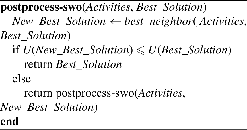
Figure 2 gives an overview of HC, as it has been applied to the problem of optimizing individual activity personal plans. U denotes the objective function of (7) and Solution and New_Solution denote complete and valid assignments to the decision variables $p_{i}$ , $t_{i j}$ , $d_{i j}$ and $l_{i j}$ . HC is initialized with the problem definition (Activities) and SWO’s output solution as the initial Best_Solution.

3.1. Computing the best neighbor

The best_neighbor function computes all neighboring solutions by applying various transformations to the current solution and returns the best one of them. HC continues until no further improvement is possible the current solution; then, the last solution is returned.

3.1.1. Best start time

This transformation attempts to reschedule each part $T_{i j}$ (with $d_{i j} > 0$ ) within $D_{i}$ . Potential gains from rescheduling $T_{i j}$ include:

$T_{i j}$ is scheduled at a more preferred time window, that is, $U_{i}^{time}$ increases.

$T_{i j}$ is scheduled at a less congested time window, so $d_{i}$ can increase (using another transformation at a later stage).

Other parts $T_{k l}$ can be scheduled at a more preferred time window or they can increase their durations, using subsequent transformations.

The transformation attempts alternative values for each decision variable $t_{i j}$ taken from its domain $D_{i}$ , one value per decision variable at a time. For each value attempted, the constraints are checked to examine if the change is consistent with them. If it is not, the value is ignored.

3.1.2. Changing the duration

This transformation attempts to change the duration of an activity part. Duration increment is a source of extra utility, but decreasing the duration of an activity part may provide extra temporal space to be exploited by subsequent transformations. HC does not accept duration decrements, since they result in a temporary utility drop; on the contrary, SA does accept them stochastically.

This transformation attempts different values for each decision variable $d_{i j}$ (with current value $d_{i j} > 0$ ), ranging between ${smin}_{i}$ and ${smax}_{i}$ . Each potential change is checked for constraint consistency.

3.1.3. Merging two parts of an activity

This transformation attempts to merge two parts of the same activity into a single part. For part $T_{i j}$ , with $d_{i j} > 0$ , it iterates over all other parts of activity $T_{i}$ , and for every $T_{i k}$ , $j \neq k$ and $d_{i k} > 0$ , it attempts to remove $T_{i k}$ from the plan and to add its duration to $T_{i j}$ . Combining two activity parts, $T_{i j}$ and $T_{i k}$ , into a single one (that is, reducing $p_{i}$ by one), provided that duration constraints are not violated, may provide temporal space for other activity parts to be scheduled, which could not fit in the schedule up to the application of this transformation.

Particularly, for every ordered pair $(T_{i j}, T_{i k})$ , $j \neq k$ , $d_{i j} > 0$ and $d_{i k} > 0$ , the transformation first checks whether $d_{i j} + d_{i k} ⩽ {smax}_{i}$ holds. In case it does, it adds $d_{i k}$ to $d_{i j}$ , sets $d_{i k} = 0$ and attempts to produce two new solutions: One in which $t_{i j}$ does not change (that is, the extra duration is added after $T_{i j}$ ) and another in which $d_{i k}$ is subtracted from $t_{i j}$ (that is, the extra duration is added before $T_{i j}$ ). As usual, every solution produced is checked for constraint consistency.

3.1.4. Transfering duration

This transformation attempts to transfer duration between two parts of the same activity. For every ordered pair of parts, $(T_{i j}, T_{i k})$ , $j \neq k$ , it attempts to transfer duration from $T_{i k}$ to $T_{i j}$ . Particularly, for every $T_{i k}$ , such as ${smin}_{i} < d_{i k}$ and $d_{i j} < {smax}_{i}$ , up to four neighboring solutions are computed:

Move the maximum possible duration, $δ d_{k j}^{i}$ , from the end of $T_{i k}$ to the end of $T_{i j}$ .

Move the maximum possible duration, $δ d_{k j}^{i}$ , from the end of $T_{i k}$ to the beginning of $T_{i j}$ . The start time of $T_{i j}$ is updated by $t_{i j} = t_{i j} - δ d_{k j}^{i}$ .

Move the maximum possible duration, $δ d_{k j}^{i}$ , from the beginning of $T_{i k}$ to the beginning of $T_{i j}$ . The start times of both parts are updated by $t_{i j} = t_{i j} - δ d_{k j}^{i}$ and $t_{i k} = t_{i k} + δ d_{k j}^{i}$ .

Move the maximum possible duration, $δ d_{k j}^{i}$ , from the beginning of $T_{i k}$ to the end of $T_{i j}$ . The start time of $T_{i k}$ is updated by $t_{i k} = t_{i k} + δ d_{k j}^{i}$ .

The maximum possible duration to move from $T_{i k}$ to $T_{i j}$ is initialized with $δ d_{k j}^{i} = min ({smax}_{i} - d_{i j}, d_{i k} - {smin}_{i})$ . In all cases, the durations of two parts are changed by $d_{i k} = d_{i k} - δ d_{k j}^{i}$ and $d_{i j} = d_{i j} + δ d_{k j}^{i}$ . If the constraint consistency check on any of the four cases fails, $δ d_{k j}^{i}$ is recursively decreased by one and the transformation is reapplied for this particular case until either a valid solution is found or $δ d_{k j}^{i} = 0$ .

3.1.5. Splitting a part

This transformation attempts to split a part into two parts. For part $T_{i j}$ , where $d_{i j} ⩾ 2 \times {smin}_{i}$ , it attempts to create a new part $T_{i k}$ where $k = p_{i} + 1$ . The new part will have $d_{i k} = {smin}_{i}$ and $l_{i k} = l_{i j}$ , whereas $d_{i j}$ is decreased by ${smin}_{i}$ . Alternative values are tried for $t_{i k}$ , trying to satisfy the problem constraints. If no valid $t_{i k}$ is found, no new solution is produced; otherwise, one solution for each possible $t_{i k}$ can be produced (HC would select the best one of them; SA would select any of them stochastically).

3.1.6. Increasing the duration of an activity

This transformation increases the duration of an activity part $T_{i j}$ and, consequently, of the whole activity $T_{i}$ , by one time unit, thus increasing $U_{i} (d_{i})$ . Particularly, for each part $T_{i j}$ , where $d_{i j} < {smax}_{i}$ and $d_{i} < d_{i}^{max}$ , it attempts to produce up to two new solutions. In both cases, $d_{i j}$ is increased by one. In the first case, $t_{i j}$ does not change, that is, the extra duration for $T_{i j}$ is added after it. In the second case, $t_{i j}$ is reduced by one, that is, the extra duration for $T_{i j}$ is added before it.

3.1.7. Swapping parts of different activities

This transformation attempts to swap the start times of two parts, $T_{i j}$ and $T_{k l}$ , $i \neq k$ . Sometimes, an increase in the overall utility is possible in this way. This swap may not be possible with the previous transformations, because it would require moving temporarily either $T_{i j}$ or $T_{k l}$ in a less preferred time window (not allowed by HC), or because there is no free space to move temporarily one of the two parts; hence the necessity to have an explicit transformation for such swaps. As usually, each potential new solution is checked for constraint consistency.

3.1.8. Adding a part

Having applied several transformations, it may be possible to add an extra part for an already scheduled activity $T_{i}$ , thus significantly increasing $U_{i} (d_{i})$ . This transformation is different from the previous ones in that it does not operate on parts but on whole activities. For each activity $T_{i}$ , with $d_{i}^{min} ⩽ d_{i} < d_{i}^{max}$ , it is attempted to add a new part in the current schedule, provided that: $\begin{matrix} (8) & d_{i} ⩽ d_{i}^{max} - {smin}_{i} \end{matrix}$ that is, adding a new part with the minimum possible duration for the pair does not exceed the maximum allowed duration $d_{i}^{max}$ for the whole activity.

For the new part $T_{i k}$ ( $k = p_{i} + 1$ ), for each possible $t_{i k}$ where the new part could be scheduled, $l_{i k}$ is greedily selected from ${Loc}_{i}$ in such a way that traveling time from the locations of the adjacent (with respect to $t_{i k}$ ) parts is minimized, whereas $d_{i k}$ is set to the maximum possible duration of part $T_{i k}$ for the specific values of $t_{i k}$ and $l_{i k}$ . The best combination of $(t_{i k}, l_{i k})$ is returned. If adding a new part is successful, $p_{i}$ is increased by one.

3.1.9. Adding an activity

Similarly to adding a part, it may be possible to add a whole new activity (that is, an activity that was not possible to be scheduled previously) to the schedule. For an activity $T_{i}$ that is not included in the current schedule, this transformation greedily tries to schedule it by inserting parts to the timeline within its domain, starting from the earliest and proceeding to the latest time points. At each time window where a part of $T_{i}$ can be inserted, it is inserted with the maximum possible duration and at the best possible location, taking into account the locations of the two already scheduled temporally adjacent activities. The transformation terminates as soon as: $\begin{matrix} (9) & \sum_{j = 1}^{p_{i}} d_{i j} ⩾ d_{i}^{min} \end{matrix}$ is satisfied. Due to the greedy strategy of this transformation, it might fail to schedule an unscheduled activity, although it was possible to schedule it.

Fig. 3.

Simulated annealing based post-processing algorithm.

3.1.10. Changing locations

Changing the location $l_{i j}$ of part $T_{i j}$ does not immediately affect the utility of a plan, since the model does not assign utilities to the alternative locations of an activity. However, it may increase the free time that is available for scheduling other activities, by reducing the time needed for traveling.

This transformation produces a new solution for every location change. Particularly, for every scheduled part $T_{i j}$ , this transformation attempts to change its location, by trying every alternative (if any) location l in ${Loc}_{i}$ . The best location selected is the one that minimizes the total traveling time of the plan. The total traveling time of a plan is calculated as the sum of all time intervals reserved for traveling between locations. In case of finding a better location for the current part, this transformation triggers all the aforementioned transformations that concern parts of scheduled activities.

3.1.11. Trimming activity parts

The aforementioned transformations work better if plenty of free time is available. There are cases though where the activities have tight domains and the post-processor has to operate upon a tight solution as its initial input. In such cases, the HC algorithm usually terminates with no solution improvement, whereas SA usually manages to improve it by first applying the Change Duration transformation and decreasing some activities’ duration.

This transformation attempts to free some time on tight plans. It is called once only on a seed solution before it is passed to the post-processor for improvement. Initially, it determines the tightness of SWO’s solution using a heuristic approach. Particularly, the utilization values of all used time slots (either for scheduled activity parts or for traveling time) is summed, and divided by the net size of the available domain for all activities. If the plan tightness is greater than a threshold (we used 0.9), trimming is applied on SWO’s solution before it is passed to the post-processor. Trimming works as follows: For every $T_{i j}$ , starting from $j = 1$ , it sets its duration $d_{i j}$ to the value $max ({smin}_{i}, d_{i j} - d_{i} + d_{i}^{min})$ , that is, to the minimum possible duration such that the total duration of $T_{i}$ becomes no less than $d_{i}^{min}$ .

3.2. Avoiding local optima

The hill-climbing post-processing algorithm can get stuck in local optima. On the other hand, simulated annealing [10] alleviates this problem by giving a chance (although with low probability) to escape from local optima. So, to advance our previous work, we replaced hill-climbing as a post-processing algorithm with simulated annealing (SA), empowered with a tabu list and backtracking.

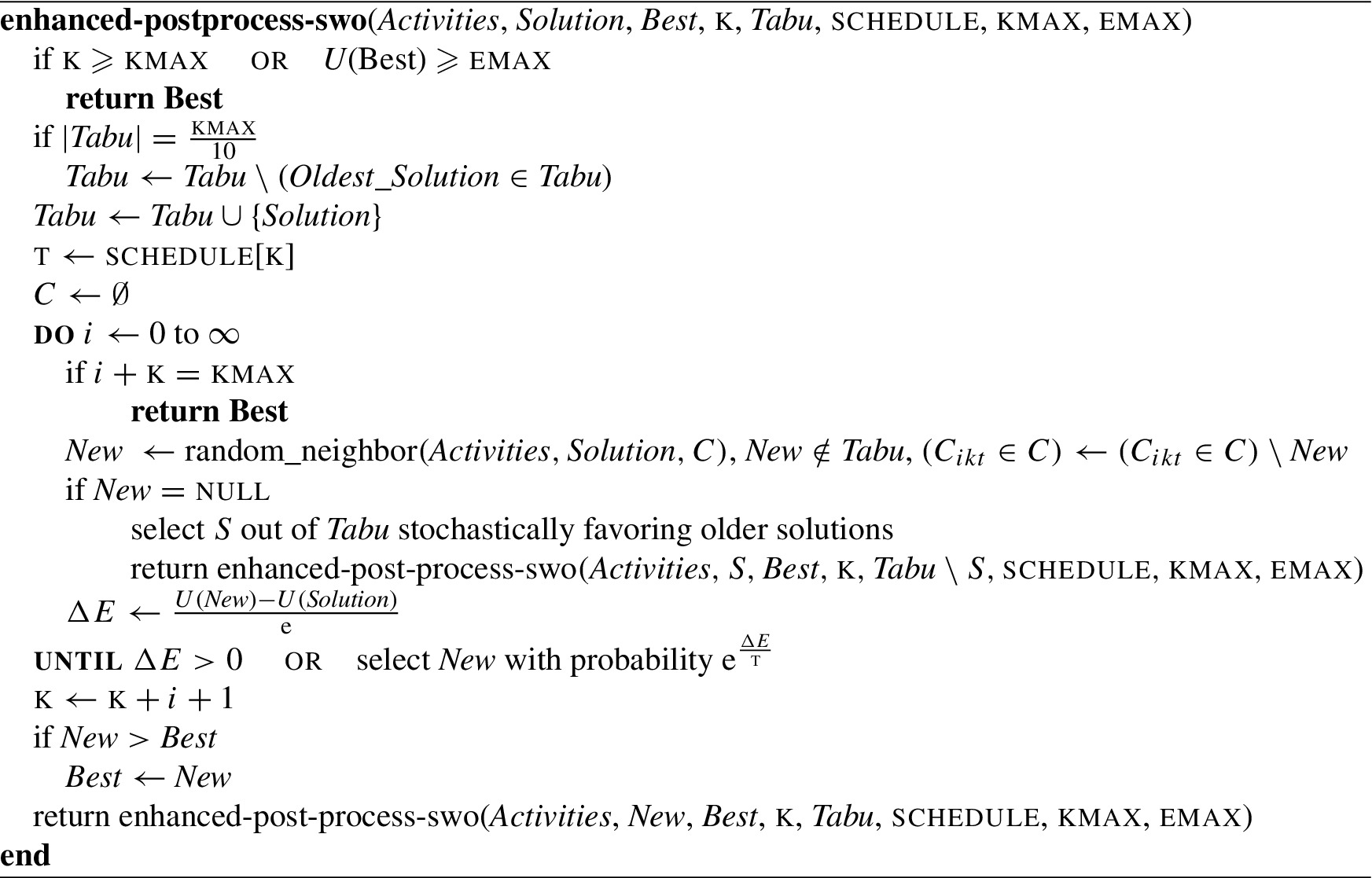
Similar to HC, SA based post-processing algorithm (Fig. 3) uses as seed the solution produced by the preceding SWO phase. The transformation functions presented in the previous section have been modified so as to return all the valid neighbor solutions, instead of just the best one. A solution is picked stochastically in four stages: First a transformation is selected, then an activity (scheduled or not scheduled, depending on the transformation) is selected, then a part of an activity is selected (if anticipated by the transformation) and, finally, all the valid neighbors for the selected transformation, activity and part of it are computed and one of them is picked.

The SA post-processing algorithm uses the random_neighbor function (instead of best_neighbor), which returns a random neighbor state. For increased efficiency, the sets of neighbor solutions created are cached as long as the randomly picked neighbor solutions are not accepted (variable $C_{i k t}$ in Fig. 3 holds the cached neighbors for activity $T_{i}$ , part $T_{i k}$ and transformation t). Thus, if one of the cached triples (transformation, activity, part) is selected in the next iteration, the set of neighbor solutions for that transformation is not generated again. Cached data are cleared as soon as a new solution is accepted. The number of valid states, for a transformation applied on a part, is not known beforehand.

If the selected variable list $C_{i k t}$ is empty, the algorithm will choose another transformation or activity part. If all the lists are empty, the search algorithm will backtrack to a previous solution, according to a probability distribution. Thus, backtracking is employed each time SA cannot find a neighbor that is not already in the tabu list. Without backtracking, such situations constitute a termination condition for SA. Backtracking selects stochastically a solution from the tabu list, giving higher probability to earlier solutions, and continues from there on. Backtracking is employed in over-constrained problems, when the size of the neighborhood decreases drastically towards the size of the tabu list.

The SA search algorithm uses four parameters: kmax, emax, schedule and $| Tabu |$ . kmax is the number of iterations of the simulated annealing algorithm and emax is the loosely computed upper bound of the utility for the problem in hand. schedule defines the cooling schedule of SA. We used a cooling schedule dependent on kmax, which is defined as: $SCHEDULE [K] = SCHEDULE [K - 1] \times (1 - 0.07 \times \frac{100}{KMAX})$ , where $SCHEDULE [1] = 0.9$ . We set the maximum value of $| Tabu |$ (the number of past states kept in the tabu list) to $\frac{KMAX}{10}$ . These values were chosen after extensive experimentation.

4. Evaluation

This section comprises an extensive evaluation of the proposed local search techniques applied to the problem of scheduling individual personal activities. First we compare the base algorithm SWO to its enhancements with either HC or SA in the post-processing phase, employing the eleven transformations presented in the previous section. We also compare SWO to SA applied to an empty plan. Then, we present a sensitivity analysis showing the contribution of each individual transformation to the performance of SA. Next we evaluate post-processing optimization on an illustrative realistic scenario. Finally, we discuss transferability issues of the evaluated computational methods.

4.1. Comparing to SWO

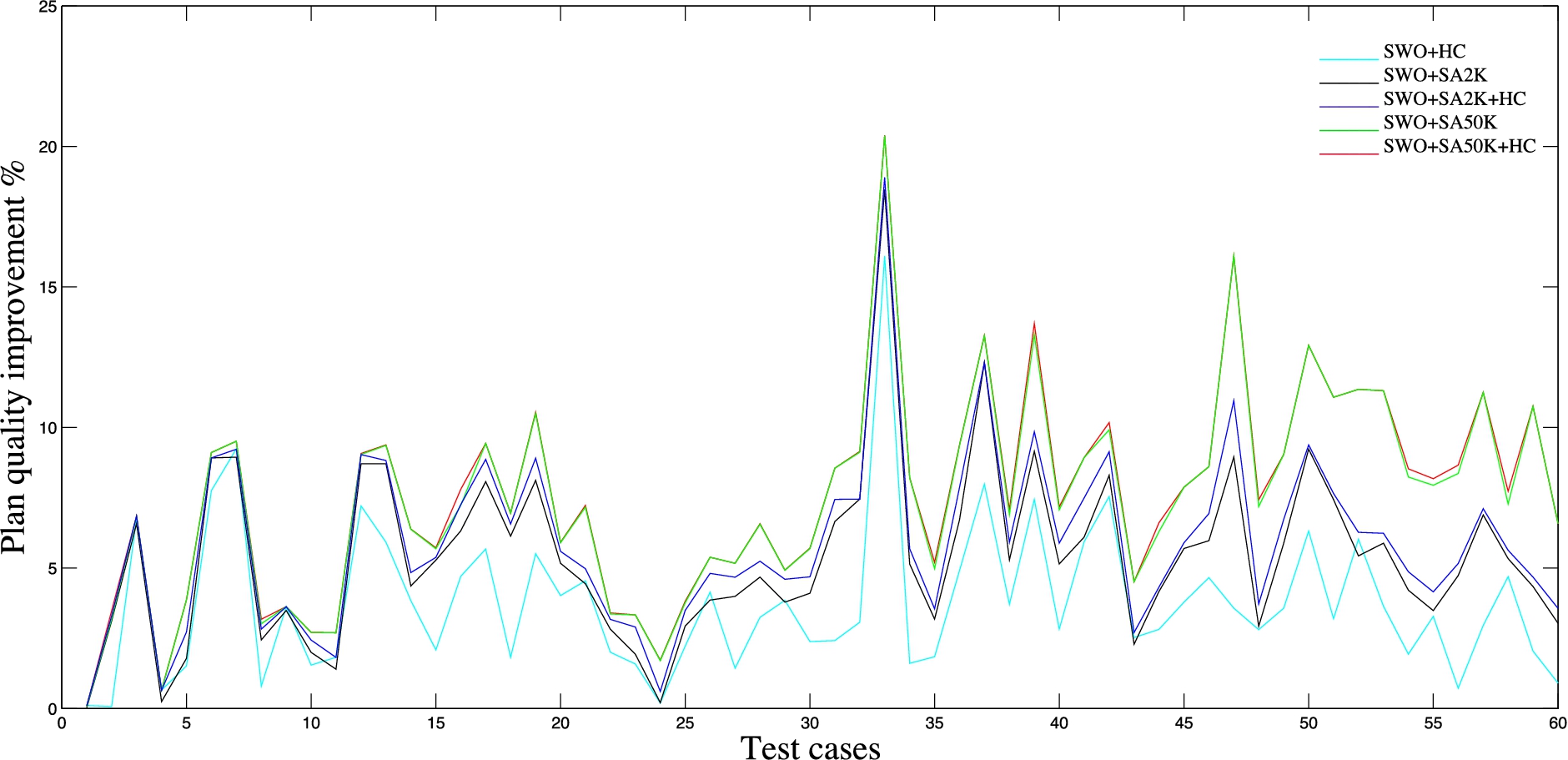
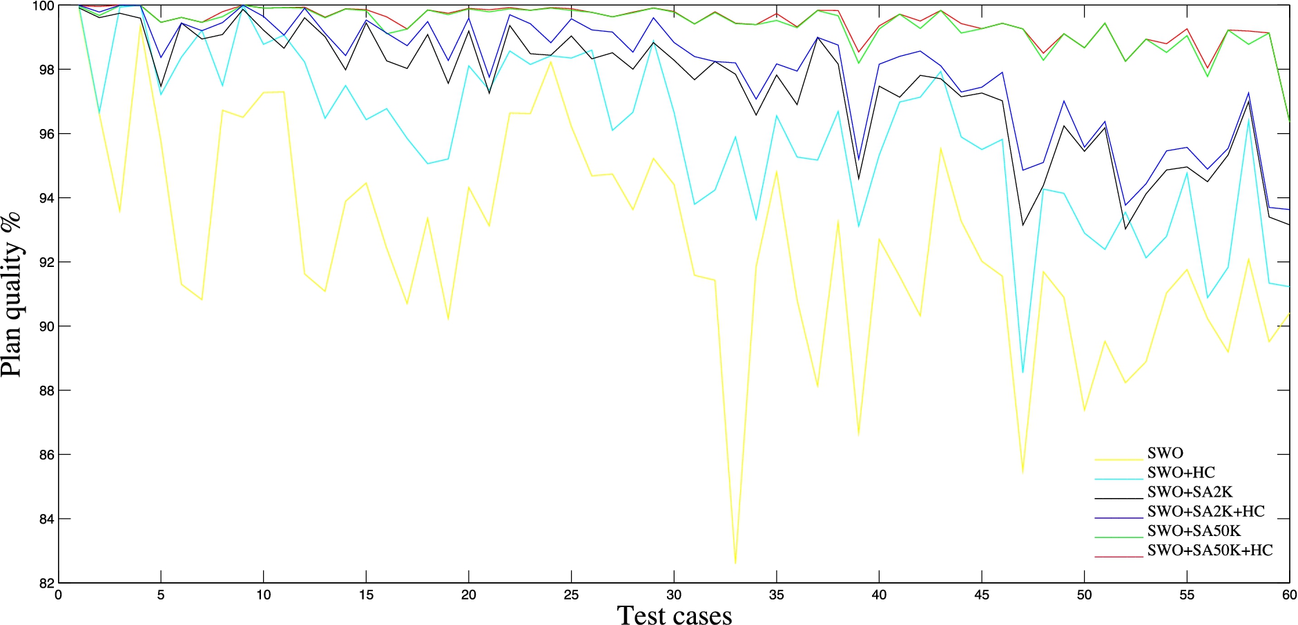
We first compare the original SWO algorithm to SWO coupled with HC at a post-processing phase, as well as to SWO coupled with SA, on $60$ test cases, ranging in size, taken from previous work [18]. All experiments involving either HC or SA were executed $10$ times and the averages are reported. The implementation of the above algorithms was done in C++ and the experiments were run on an Intel Xeon 2.66 GHz processor.

Fig. 4.

Improvement of plan quality over SWO. (Colors are visible in the online version of the article; https://dx-doi-org.web.bisu.edu.cn/10.3233/AIC-150680.)

According to the literature [18], the problems in the test suite differ only in the number of activities, whereas the rest of the parameters are constant. The planning horizon is set to 500 time units for all problems, with the temporal domain of each activity being a random set of intervals covering the entire planning horizon. 70% of the activities have fixed duration. 40% of the activities are interruptible with minimum distance constraints, 30% of these have maximum distance constraints, 30% have minimum distance preferences and 30% have maximum distance preference. 20% of the activities have utilization 0.5; the rest have full utilization. Binary constraints and preferences are defined with probability $1 / (2 N)$ for every pair of activities and every type of constraint or preference. There are 4 locations, with random subsets of them assigned to the activities. Activity utilities are selected from the interval $[5, 12]$ , temporal preference utilities from the interval $[5, 10]$ and duration utilities from the interval $[2, 5]$ . All utilities assigned to binary preferences are selected from the interval $[1, 3]$ .

The results of the first comparison are shown in Fig. 4. The plot represents the plan quality percentage improvement of the post-processing algorithms to the original SWO. We explored five post processing configurations: SWO followed by HC (denoted with SWO+HC); SWO followed by SA running for 2,000 iterations (denoted with SWO+SA2K); SWO+SA2K followed by HC, in order to reach the nearest local maximum (denoted with SWO+SA2K+HC); SWO followed by SA running for 50,000 iterations (denoted with SWO+SA50K); and, finally, SWO+SA50K followed by HC (denoted with SWO+SA50K+HC).

As we can observe from Fig. 4, there is an improvement in all test cases with the less aggressive configurations SWO+HC and SWO+SA2K. The best case was a 18.46% improvement in plan quality with SWO+SA2K. The average improvement was 3.75% for SWO+HC and 5.37% for SWO+SA2K. SWO+SA2K+HC’s improvement over SWO was 5.89% on average. Concerning the more aggressive configurations, SWO+SA50K+HC improves over SWO 7.51% on average, with a best case of 20.38%, whereas SWO+SA50K’s average improvement was 7.48%, with a best case of 20.37%.

Figure 5 compares the run-time of the algorithms. The figure is in logarithmic (base 10) scale, with the yellow line representing SWO as the base case. Concerning the less aggressive configurations (SWO+SA2K and SWO+HC) on relatively small instances, that is, with up to 20 activities, the run-times of them are similar. On larger instances, SWO+SA2K outperforms SWO+HC in terms of run-time, whereas simultaneously it provides better quality results as it has been shown in Fig. 4. Having in mind real-world situations, we consider the time requirements acceptable, since the problems of the test set are artificially created with increased complexity (many binary constraints and preferences), thus they are more complex than typical real-world situations that are expected to involve less activities with few interdependencies between them.

Fig. 5.

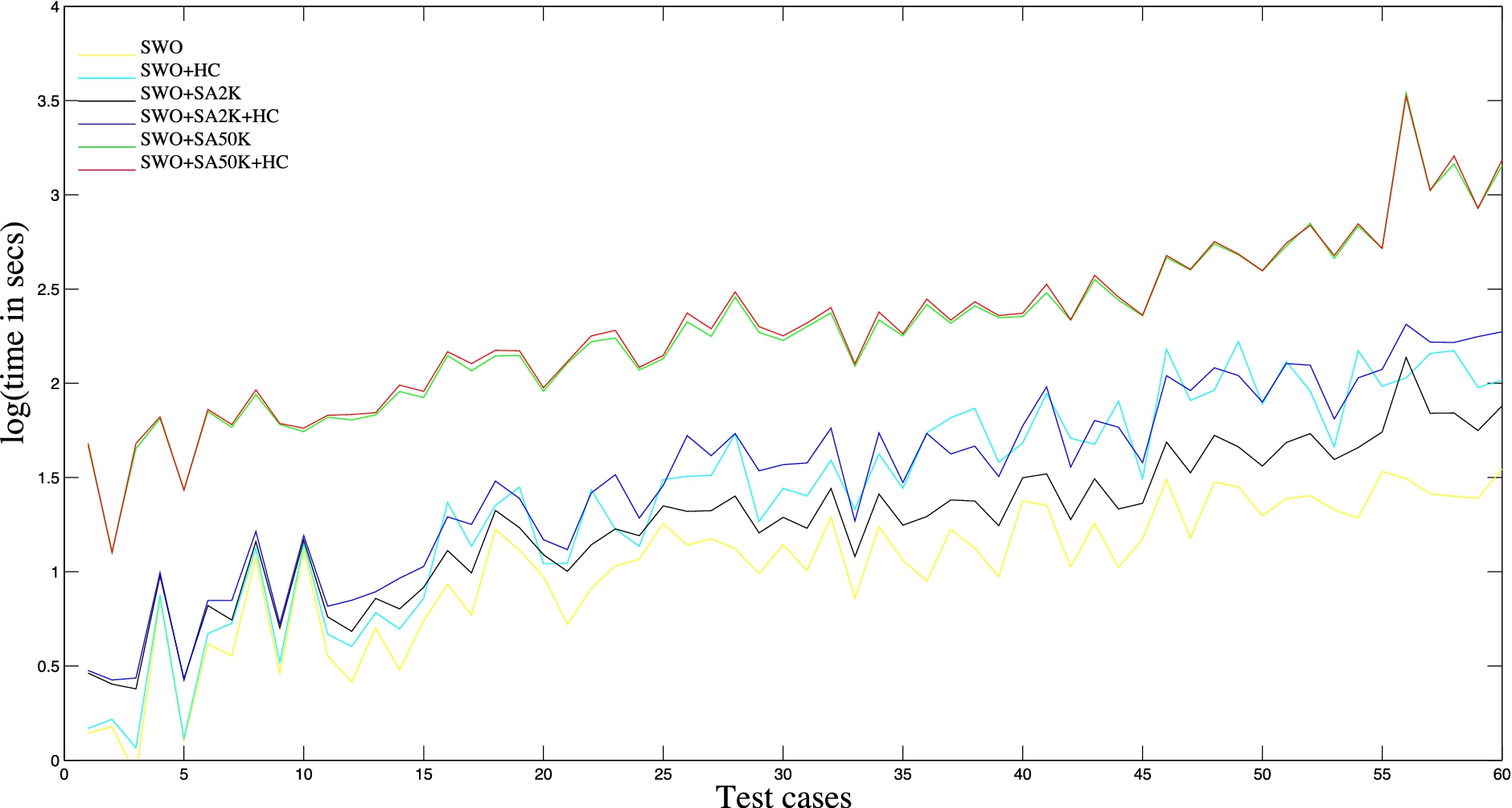
Execution time results. (Colors are visible in the online version of the article; https://dx-doi-org.web.bisu.edu.cn/10.3233/AIC-150680.)

Fig. 6.

Quality relative to the experimental upper bound. (Colors are visible in the online version of the article; https://dx-doi-org.web.bisu.edu.cn/10.3233/AIC-150680.)

Fig. 7.

Running SA from the empty plan for the same time as SWO. Quality relative to the experimental upper bound. (Colors are visible in the online version of the article; https://dx-doi-org.web.bisu.edu.cn/10.3233/AIC-150680.)

Concerning the more aggressive configurations, SWO+SA50K and SWO+SA50K+HC have similar run-times, since there are not many chances for further improvement after running SA for 50K steps. Finally, SWO+SA2K+HC is on average 114% more time demanding than SWO+SA2K.

In addition, we compared the performance of the above algorithms to the experimental upper bound of the various problem instances. The experimental upper bound was computed by running the SWO+SA50K+HC algorithm 170 times on the test set and obtaining the utility of the best solution found for each problem instance. These results are shown in Fig. 6. Particularly, SWO had an average plan quality of 92.58% to the experimental upper bound, whereas SWO+HC and SWO+SA2K had 95.99% and 97.47%, respectively. Coupling SA with HC resulted in less than 1% of average improvement relative to SA (97.94%), whereas increasing kmax raised it to 99.39%.

The worst case for SWO had a plan quality of 82.59%, which was increased to 95.89% with SWO+HC, and to 97.84% with SWO+SA2K. SWO+SA50K+HC further raised it to 99.43% on average.

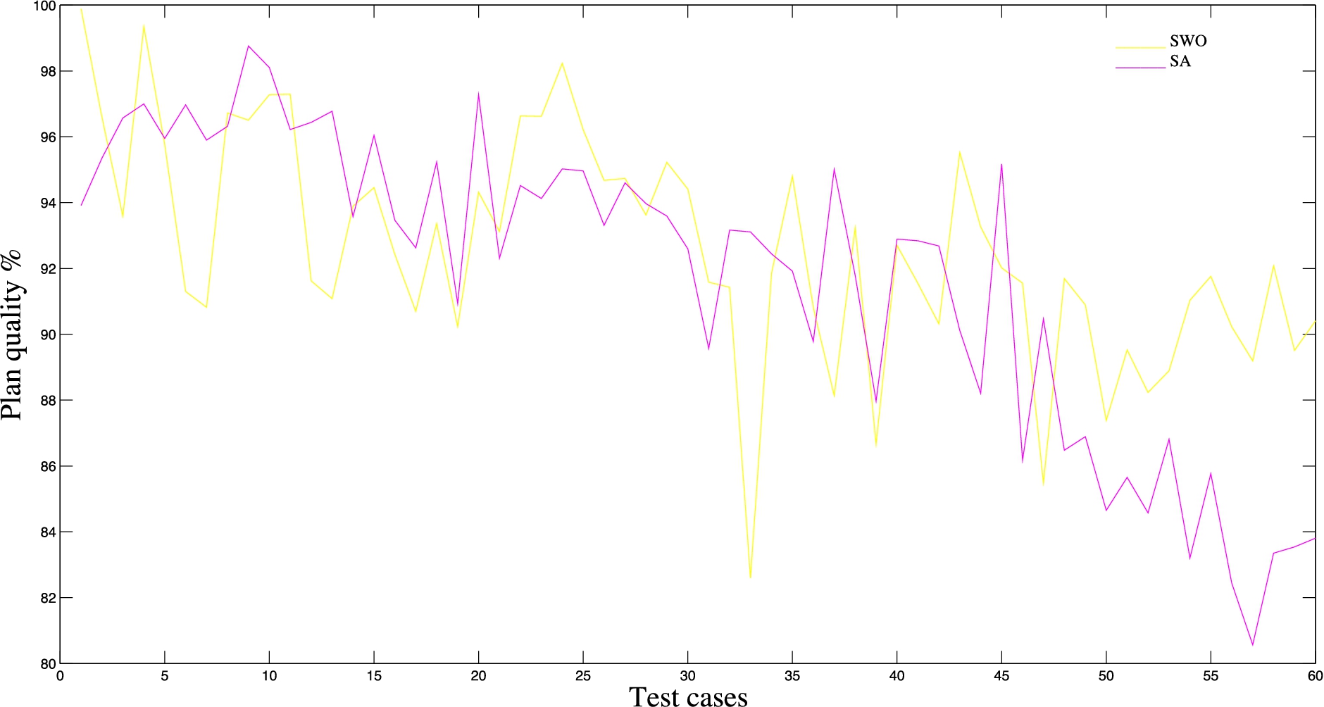
Finally, we ran SA as the only scheduler, that is, applying it to the empty plan, for all test cases. We did not use a predefined kmax value for this test (as we did in the other experiments), but we adopted as a termination criterion the run time $t_{i}^{SWO}$ spent by SWO on problem instance i, using the same settings as in the previous work [18]. The results, compared to the experimental upper bound, are shown in Fig. 7. The average utility of the SWO runs is 92.58%, whereas the average utility of the SA runs is 91.72%. As it can be seen, SA is competitive to SWO for small problems, however SWO clearly wins on the hard problem instances. Thus, running first SWO and then SA in a post-processing phase is a dominant strategy compared to running SA from the beginning, when applied to hard problems.

Additional experiments have shown that by giving more time to SWO (compared to the settings used in previous work [18]) no improvement is noticed; thus, employing stochastic local search in a post-processing phase is the only option to further optimize these plans, provided that more time is available. After thorough investigation of SWO’s behavior we realized that the main obstacle for SWO is that it searches in two coupled spaces, that is, the priority space and the solution space (Fig. 1(b)). Not every solution in the solution space has a corresponding ordering of the activities in the priority space. So, many interesting solutions cannot be reached by pure SWO, thus why the need to couple SWO with a post-processing search algorithm.

Fig. 8.

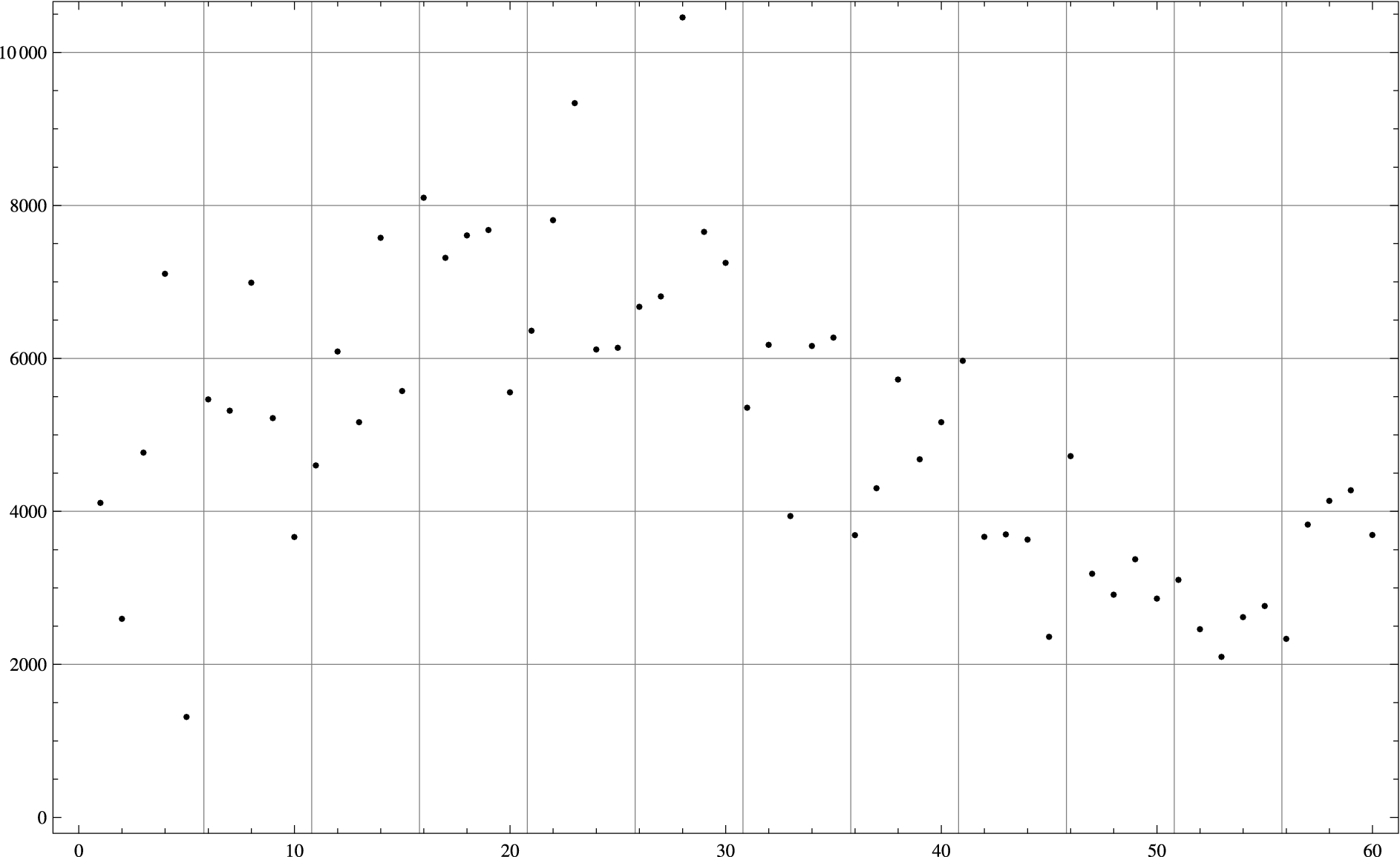
Average neighborhood size for each test case.

Fig. 9.

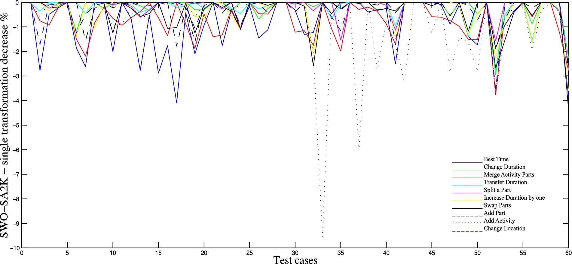
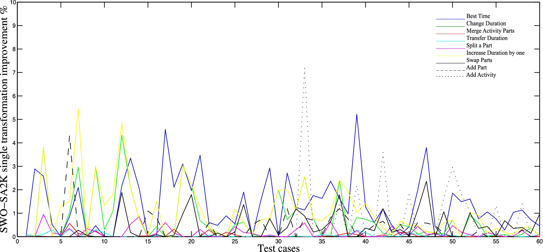
Percentage decrease in the quality of the resulting plans when nine out of the 10 transformations are employed. Each line corresponds to removing a single transformation from their bundle. (Colors are visible in the online version of the article; https://dx-doi-org.web.bisu.edu.cn/10.3233/AIC-150680.)

Fig. 10.

Percentage increase in the quality of the resulting plans when each transformation is employed separately. Each line corresponds to a single transformation being employed. (Colors are visible in the online version of the article; https://dx-doi-org.web.bisu.edu.cn/10.3233/AIC-150680.)

4.2. On the size of the neighborhood

The average neighborhood size for the 60 problem instances was computed using the SWO+SA2K+HC configuration of the scheduler. Since SA does not compute all the neighbors of a solution, we used HC’s $best_neighbor$ function, which tries every transformation that can be applied to a solution. The reported values are averages over all iterations of HC, 10 times per problem.

The results are presented in Fig. 8. The problem instances with 25 and 30 activities have the largest neighborhood size. For problems with fewer activities, the neighborhood size is smaller as expected. For problems with more activities within the same time horizon, the neighborhood size is again smaller due to the complex interactions between the activities that render many transformations invalid.

4.3. Contribution of individual transformations

Using SWO+SA2K as our basic configuration, we removed transformations from the post-processor, one of them at a time. In Fig. 9 we compare each transformation’s contribution, based on the transformations’ absence from SWO+SA2K.

The top line (0%) represents the total utility of the solutions produced by SWO+SA2K, whereas for each transformation we see the percentage decrement from SWO+SA2K, when that transformation is omitted from the post-processor. The results vary depending on the problem instance. For example, test cases #52 and #60 (hard problems) demonstrate a large drop in total utility when removing any one of the transformations, whereas in other cases removing a single transformation produces minor reduction in the total utility of the resulting solutions. These results of course depend also on the improvement that SA2K induced over the seed solution produced by SWO. The fact that by removing any one of the transformations we get a drop in the quality of the produced solutions demonstrates that the synergy of all transformation is significant in the post-processing phase. The transformation Add Activity was not always applicable, but when it was its removal gave us large drops in total utility, as should be expected.

In Fig. 10 we compare a minimal version of the SWO+SA2K with just a single transformation employed. Each transformation was tested separately to obtain a view of its contribution when used by itself. The only transformation not tested was Location Changes, as it relies on its combination with other transformations to alter the utility of a schedule, and does not modify the total utility by itself. The baseline represents SWO.

Some transformations managed to increase the total utility without relying on synergies with others. The most significant seem to be Best Start, that is, moving activity parts in the schedule and altering their $U (time)$ utility bonus, and Increase Duration by one, that is, increasing an activity part’s duration by one time unit. Other transformations did not provide any benefit when used alone. For example, Merge Activity Parts does not seem to do much by itself, there were few cases where it provided a contribution to the solution quality. Others, such as Add Activity, did not contribute anything by themselves in most test cases, but when they did they provided a huge boost in utility.

4.4. A realistic scenario

In this section we compare SWO+SA50K against SWO on a realistic scenario. The motivation is two-fold: First, to demonstrate the effectiveness of post-processing on a realistic problem and, second, to visualize the improvement incurred by post-processing over the seed plan. The scenario comprises an over-constrained problem; however, such scenarios are typical of busy people, who are reasonably expected to be interested in using intelligent assistance in managing their activities. In the following paragraphs we first describe the scenario informally, then we compare the two algorithms and finally we discuss their relative performance.

The scenario has as follows: Ann is a university teacher, with a tight weekly schedule. In addition to her regular commitments (that is, teaching, student hours, etc.), this particular week she has five additional activities. Her regular working hours are 09:00 to 19:00, Monday to Friday. On this Friday morning however she is traveling to a conference abroad, in order to present a technical paper.

Her first two activities concern preparing educational material for two of her classes (Module A and Module B). For each one of these activities Ann needs at least two hours, in case she will exploit as much as possible from last year’s material, and at most six hours, if she is going to prepare entirely new material. The extra duration, for the preparation of new material, has a high utility for her. Ann prefers to work on these activities during the evenings. The activities are interruptible; whenever Ann works on anyone of them, she should not spend less than one hour or more than two hours on it.

The third activity concerns preparing slides for the conference presentation. She wants to spend at least three hours on this activity, whereas spending two more hours might result in a more attractive presentation and, consequently, more utility for herself. Preparing the slides is a task better accomplished in the morning, whereas again the activity can be scheduled in parts of between one and two hours. The deadline of course is before the scheduled talk at the conference.

The fourth activity concerns participating at a meeting with a colleague, requiring physical presence at a nearby location that is approximately one hour away. Her colleague expects Ann either on Monday evening (between 17:00–19:00) or Tuesday afternoon (between 12:00–15:00), depending on Ann’s availability. The estimated duration of the meeting is between one and two hours, however this activity has a low utility for Ann, so she is not enthusiastic about spending more time for the meeting.

The fifth activity concerns finishing and submitting an article for a journal special issue. This is a very important task for Ann, since she is working on the article for the last two months. She expects to spend at least three hours to finish the article; however, having another last read of the text would require six hours in total (high utility). Writing the article needs large compact periods of time, of at least one and a half hours and at most three hours. Since this activity requires her complete focus, Ann prefers to accomplish writing the article within a temporal period of at most 24 hours (low utility), whereas she also prefers to schedule it as early in a day as possible. She can only work on this activity though after the meeting with her colleague (ordering constraint), since the article concerns the project they are working on together.

Regular activities involve five lectures of two hours each, which Ann is giving to her classes, in a pre-determined schedule; the regular one-hour weekly meeting with her PhD student, which can be scheduled between 13:00 and 18:00 on Thursday; a meeting with her colleagues at her Department (this is a fixed time commitment); weekly students hours, requiring two to three hours, that should be scheduled on Tuesday morning, between 9:00 and 13:00 (the utility of the extra duration is low); and, finally, daily afternoon lunches, to be scheduled between 15:00 and 17:00, having duration between half an hour and one full hour (again, the extra utility from having a long lunch is low).

The loose upper bound of the problem, that is, if all activities are scheduled with maximum duration and at their best possible intervals, was calculated to be 2,473.47. A solution of that utility can easily be shown as unattainable, due to the over-constrained nature of the problem, as the available time is less that the sum of the maximum durations of all involved activities. Furthermore, there are conflicting temporal preferences, Ann needs some time to travel to the location of the fourth activity and come back, whereas there are additional constraints such as the fifth activity’s maximum proximity preference. The experimental upper bound was found to be 2,082.2. This was calculated by running SWO+SA50K+HC 1,000 times on the problem.

SWO’s solution has a utility of 1,831.53, whereas SWO+SA50K’s solution has a utility of 2,074.09 (average over 100 runs), which is an improvement of 13.24% over SWO’s. The two solutions are outlined in Figs 11 and 12. Since the post-processor is a stochastic algorithm, we executed it 100 times on Ann’s problem and selected to present in Fig. 12 the mode (most common) solution. The “meeting with colleague” activity is denoted with different color, because it is scheduled at a different location (that is, colleague’s office) than Ann’s university. The average time required by SWO+SA50K is 12 seconds on our system, which we consider acceptable. In contrast, SWO solved the problem in 0.1 seconds.

Fig. 11.

SWO’s solution. (Colors are visible in the online version of the article; https://dx-doi-org.web.bisu.edu.cn/10.3233/AIC-150680.)

Fig. 12.

SWO+SA50K’s solution. (Colors are visible in the online version of the article; https://dx-doi-org.web.bisu.edu.cn/10.3233/AIC-150680.)

SWO (Fig. 11) omitted two activities from the plan, that is “Module A preparation” and “Meeting with PhD student”. The post-processor added these activities and returned a schedule with all seventeen activities included. Monday morning 9:00–10:00 was left unused by both algorithms, as the current time (that is, when the problem is solved) was considered to be Monday morning at 09:30 and there is no activity that can be broken into thirty minute parts and be scheduled at that time. Similarly, intervals 11:00–12:00 and 13:00–14:00 on Tuesday are used as the traveling time from Ann’s university to her colleague’s office and back. However, SWO resulted in three more unused half-hour intervals, on Monday, on Wednesday and on Thursday, that could not be used for any activity parts due to their short length.

Let’s have a deeper look at the plan found by SWO. On Monday SWO placed two parts of “Prepare slides” next to each other, so the unused space was necessary as parts of the same activity must have at least 30 min temporal distance to each other (proximity constraint). The unused space on Wednesday cannot be used by either “Prepare slides” or “Submit article” activities, since both adjacent activities are already scheduled with their maximum duration. The same is also true for the unused space on Thursday, since the lecture is a fixed-time commitment, whereas “Submit article” is already scheduled at its maximum duration (at a total time of 6 hours).

Taking this schedule of Fig. 11 as its seed solution, SWO+SA50K produced the schedule shown in Fig. 12. There are no unused intervals in the improved schedule, whereas all activities are now scheduled, even if not with their maximum duration. On Monday there is a single part of “Prepare slides”, thus making room for another part of “Module B preparation” and allowing for an one hour lunch. The total duration of “Prepare slides” has been decreased by an hour. On Tuesday, “Module B preparation” was decreased to one hour, and a part for “Module A preparation” was scheduled in the resulting free space. On Wednesday, the post-processor utilized the half-an-hour available duration out of the one-hour one it had gained for “Prepare slides” (by removing the one-hour part on Monday) to expand that activity to fill in the unused space. The rest of that day’s schedule is unaltered. Finally, on Thursday, the two “Submit article” parts were swapped and the first one was moved earlier to fill in the unused space. The afternoon lunch was decreased to half-an-hour and the “Meeting with PhD student” was added in the resulting free space. At the 18:00–19:00 interval “Module B preparation” was replaced by “Module A preparation”.

Activity “Finish article” gives the highest utility per unit of extra duration, so both schedules included it with its maximum duration (6 hours). In Fig. 12 we can observe that the allocated duration for “Prepare slides” was decreased by half-an-hour compared to Fig. 11, whereas the duration of “Module B preparation” was decreased by one hour. The one and a half hours freed, together with the one and a half hours of unused temporal space of Fig. 11, were used for adding the two extra activities, that is, two hours for “Module A preparation” and one hour for “Meeting with PhD student”.

One could argue that the post-processor should have freed one hour from “Prepare slides” and half-an-hour from “Module B preparation”, as the extra duration for Module B is more important. But, the space was needed mostly for “Module A preparation”, which has a higher utility for evening times, the same as module B, thus gaining utility from its temporal placement. Moreover, “Meeting with PhD student” had a small available domain (could only be scheduled between 13:00–18:00 on Thursday with no other temporal preference).

It is important to emphasize that the solution presented in Fig. 12 is not the best solution found by the post-optimization process; as we noted earlier, this is the most-common solution found over 100 runs, with a utility of 2,074.09, whereas the best solution found had a utility of 2,082.2. A user trying to manually improve the seed solution may occasionally find a better solution than the one suggested by the system. However, manually optimizing the seed solution could not be adopted as a regular practice, since it requires significant human effort, especially by inexperienced users. For example, by comparing the plans before and after applying post-optimization to the realistic scenario, we count more than ten activity parts that have been changed with at least one transformation. In this way we justify the need for intelligent solutions to produce optimized personal plans, such as the one presented in this article.

4.5. On the contribution of trimming and backtracking in over-constrained problems

Trimming and backtracking are two techniques that are employed in over-constrained problems only. Since the realistic scenario is such a problem, it is interesting to have a closer view at their contribution (separately and jointly) to the outcome of the post-processing optimization. Neither backtracking nor trimming have any effect on the rest of the problems of our test suite, since even the tight problems with 60 activities are not over-constrained.

Table 1
SWO+SA50K 100 runs

Backtracking Trimming Utility average St. deviation

ON ON 2,074.30 3.0863

OFF ON 2,049.21 37.4489

ON OFF 1,997.27 41.7054

OFF OFF 1,861.80 17.0797

Backtracking	Trimming	Utility average	St. deviation
ON	ON	2,074.30	3.0863
OFF	ON	2,049.21	37.4489
ON	OFF	1,997.27	41.7054
OFF	OFF	1,861.80	17.0797

Table 1 presents aggregated results of the post-optimization phase over 100 runs on the realistic scenario, with four configurations: (a) with backtracking, with trimming, (b) without backtracking, with trimming, (c) with backtracking, without trimming, and (d) without backtracking, without trimming. As it is clear from the results, post-optimization in over-constrained problems, enhanced with trimming and backtracking, produces steadily better results with negligible deviation, compared to not using either trimming or backtracking or both. By having a closer look at the data, we notice that trimming is more important than backtracking, producing better average results with lower deviation. However, their combination is by far better, both in terms of utility, as (most significantly) in terms of deviation.

4.6. Discussion

The approach followed in this work can be applied to other constraint optimization problems (COP) as well, particularly in project scheduling applications. The first step is to define in-domain characteristics of the problem, that affect the overall utility of a solution, and exploit them to produce a reasonable set of transformations to compute the neighborhood of any solution.

A transformation may be defined over a single decision variable, but can affect other decision variables as well. A transformation may decrease the value of the objective function; however, this would allow subsequent transformations to increase it further. Transformations should be evaluated both in isolation, as well as in combination to each other. Transformations with no apparent and distinct contribution to the overall local search optimization process should be abandoned.

Hierarchical neighborhood exploration is another novel feature of the proposed work. In order to find a neighbor, first one major decision has to be made, such as what activity to alter. Then, the type of transformation has to be selected. Depending on the type, another decision might be necessary, i.e., which part of the activity to alter. Finally, all the valid values for the involved decision variable are generated and one of them is selected stochastically. Neither the number of the valid neighbors, nor its upper-bound, need to be known.

Hierarchical neighborhood can be combined with caching subsets of neighbors. The first time a specific combination of activity, transformation and part of activity is encountered, the set of valid values for the involved decision variable can be cached. Note that extracting the set of valid values for a specific decision variable is a time demanding process. So, the next time the same combination is encountered, without having accepted any neighbor in the between, valid neighbors can be retrieved from the cache, thus accelerating SA significantly, especially during the last stages of its execution, when accepting a neighbor occurs less often.

5. Summary and future work

In this article we employed local search optimization methods to further improve the quality of individual activity personal plans with complex constraints and preferences, that were originally produced by an adaptation of the squeaky wheel optimization framework. Due to the complexity and interplay of the constraint optimization model, local search seems to be a necessity to obtain locally optimal plans.

Based on extensive experimental results, we found two practical configurations of the proposed post-optimization modules: The first one, which is optimized for speed, consists of a simulated annealing post-processing phase with a predefined moderate number of iterations. The second one, which is optimized for utility, couples an extended simulated annealing phase with a hill-climbing one. Local search is based on a series of transformations over the schedules, resulting in a large neighborhood. As demonstrated in the article, all transformations, either independently or jointly, have a value in getting qualitative solutions. Furthermore, we showed that similar results can be achieved by employing local search techniques only, i.e., using the empty plan as the start point. A real-world scenario was also employed to demonstrate the effectiveness of the proposed local search methods, presenting the schedules before and after post-optimization in the familiar calendar form.

For the future, we are considering further enhancements to both the model and the scheduling algorithm. Concerning the model, we are working on supporting joint activities, that is, activities where many persons are involved. We are also considering to support preferences over alternative locations for each activity. Our ultimate goal is to convert the constraint optimization problem to a planning problem, with activities having preconditions and effects, thus allowing for intelligent agent assistants that proactively add tasks into a user’s task list.

Concerning the algorithms, we are working on devising new transformations for exploring the local neighborhood, including pre-specified combinations of the transformations presented in this article. Using heuristics to select a subset of the transformations to consider might be of great significance, in order to keep the whole approach efficient.

Footnotes

Acknowledgements

The authors are supported for this work by the European Union and the Greek Ministry of Education, Lifelong Learning and Religions, under the program “Competitiveness and Enterprising” for the areas of Macedonia–Thrace, action “Cooperation 2009”, project “A Personalized System to Plan Cultural Paths (myVisitPlanner^GR)”, code: 09SYN-62-1129.

References

[1]

Alexiadis and

Refanidis, Meeting the objectives of personal activity scheduling through post-optimization, in: First International Workshop on Search Strategies and Non-standard Objectives (SSNOWorkshop’12), in Conjunction with CPAIOR’2012, Nantes, France, May 2012, 2012.

[2]

Alexiadis and

Refanidis, Post-optimizing individual activity plans through local search, in: Proceedings of ICAPS 2013 Workshop on Constraint Satisfaction Techniques for Planning and Scheduling Problems (COPLAS), 2013, pp. 7–15.

[3]

Bank,

Cain,

Shoham,

Suen and

Ariely, Turning personal calendars into scheduling assistants, in: Proceedings of the 2012 ACM Annual Conference Extended Abstracts on Human Factors in Computing Systems Extended Abstracts, CHI EA’12, ACM, New York, NY, USA, 2012, pp. 2667–2672.

[4]

P.M.

Berry,

Gervasio,

Peintner and

Yorke-Smith, PTIME: Personalized assistance for calendaring, ACM Transactions on Intelligent Systems and Technology 2(4) (2011), 40.

[5]

Chrpa,

T.L.

McCluskey and

Osborne, Optimizing plans through analysis of action dependencies and independencies, in: ICAPS,

McCluskey,

Williams,

J.R.

Silva and

Bonet, eds, AAAI Press, 2012.

[6]

Curran,

Freuder and

Jansen, Incremental evolution of local search heuristics, in: Proceedings of the 12th Annual Conference on Genetic and Evolutionary Computation, GECCO’10, ACM, New York, NY, USA, 2010, pp. 981–982.

[7]

Freed,

Carbonell,

Gordon,

Hayes,

Myers,

Siewiorek,

Smith,

Steinfeld and

Tomasic, Radar: A personal assistant that learns to reduce email overload, in: Proceedings of the 23rd National Conference on Artificial Intelligence, AAAI’08, Vol. 3, AAAI Press, 2008, pp. 1287–1293.

[8]

Ingber, Simulated annealing: Practice versus theory, Mathematical and Computer Modelling 18(11) (1993), 29–57.

[9]

Joslin and

D.P.

Clements, Squeaky wheel optimization, Journal of Artificial Intelligence Research 10 (1999), 353–373.

10.

[10]

Kirkpatrick,

C.D.

Gelatt and

M.P.

Vecchi, Optimization by simulated annealing, Science 220 (1983), 671–680.

11.

[11]

H.-J.

Lee,

S.-J.

Cha,

Y.-H.

Yu and

G.-S.

Jo, Large neighborhood search using constraint satisfaction techniques in vehicle routing problem, in: Advances in Artificial Intelligence,

Gao and

Japkowicz, eds, Lecture Notes in Computer Science, Vol. 5549, Springer, Berlin, Heidelberg, 2009, pp. 229–232.

12.

[12]

K.L.

Myers,

Berry,

Blythe,

Conley,

M.T.

Gervasio,

D.L.

McGuinness,

D.N.

Morley,

Pfeffer,

M.E.

Pollack and

Tambe, An intelligent personal assistant for task and time management, AI Magazine 28(2) (2007), 47–61.

13.

[13]

Nakhost and

Müller, Action elimination and plan neighborhood graph search: Two algorithms for plan improvement, in: ICAPS,

R.I.

Brafman,

Geffner,

Hoffmann and

H.A.

Kautz, eds, AAAI Press, 2010, pp. 121–128.

14.

[14]

Palen, Social, individual and technological issues for groupware calendar systems, in: Proceedings of the SIGCHI Conference on Human Factors in Computing Systems: The CHI Is the Limit, CHI’99, ACM, New York, NY, USA, 1999, pp. 17–24.

15.

[15]

Refanidis, Managing personal tasks with time constraints and preferences, in: ICAPS,

M.S.

Boddy,

Fox and

Thiébaux, eds, AAAI Press, 2007, pp. 272–279.

16.

[16]

Refanidis and

Alexiadis, Deployment and evaluation of SelfPlanner, an automated individual task management system, Computational Intelligence 27(1) (2011), 41–59.

17.

[17]

Refanidis,

Emmanouilidis,

Sakellariou,

Alexiadis,

R.-A.

Koutsiamanis,

Agnantis,

Tasidou,

Kokkoras and

P.S.

Efraimidis, myVisitPlanner^GR: Personalized itinerary planning system for tourism, in: SETN,

Likas,

Blekas and

Kalles, eds, Lecture Notes in Computer Science, Vol. 8445, Springer, 2014, pp. 615–629.

18.

[18]

Refanidis and

Yorke-Smith, A constraint-based approach to scheduling an individual’s activities, ACM Transactions on Intelligent Systems and Technology 1(2) (2010), 12.

19.

[19]

Schöning, Comparing two stochastic local search algorithms for constraint satisfaction problems, in: Computer Science – Theory and Applications,

Ablayev and

Mayr, eds, Lecture Notes in Computer Science, Vol. 6072, Springer, Berlin, Heidelberg, 2010, pp. 344–349.

20.

[20]

Selman,

Kautz and

Cohen, Local Search Strategies for Satisfiability Testing, DIMACS: Series in Discrete Mathematics and Theoretical Computer Science, 1995, pp. 521–532.

Optimizing individual activity personal plans through local search

Abstract

Keywords

1. Introduction

2. Background

2.1. Problem formulation

2.3. Usability issues

3. Applying local search methods to improve SWO output

3.1.1. Best start time

3.1.2. Changing the duration

3.1.3. Merging two parts of an activity

3.1.4. Transfering duration

3.1.5. Splitting a part

3.1.6. Increasing the duration of an activity

3.1.7. Swapping parts of different activities

3.1.8. Adding a part

3.1.9. Adding an activity

3.1.11. Trimming activity parts

3.2. Avoiding local optima

4. Evaluation

4.1. Comparing to SWO

4.3. Contribution of individual transformations

4.4. A realistic scenario

Table 1 SWO+SA50K 100 runs Backtracking Trimming Utility average St. deviation ON ON 2,074.30 3.0863 OFF ON 2,049.21 37.4489 ON OFF 1,997.27 41.7054 OFF OFF 1,861.80 17.0797

5. Summary and future work

Footnotes

Acknowledgements

References

Table 1
SWO+SA50K 100 runs

Backtracking Trimming Utility average St. deviation

ON ON 2,074.30 3.0863

OFF ON 2,049.21 37.4489

ON OFF 1,997.27 41.7054

OFF OFF 1,861.80 17.0797