A machine learning pipeline for extracting decision-support features from traffic scenes 1

Abstract

Traffic systems play a key role in modern society. However, these systems are increasingly suffering from problems, such as congestions. A well-known way to efficiently reduce this kind of problem is to perform traffic light control intelligently through reinforcement learning (RL) algorithms. In this context, extracting relevant features from the traffic environment to support decision-making becomes a central concern. Examples of such features include vehicle counting on each queue, identification of vehicles’ origins and destinations, among others. Recently, the advent of deep learning has paved to way to efficient methods for extracting some of the aforementioned features. However, the problem of identifying vehicles and their origins and destinations within an intersection has not been fully addressed in the literature, even though such information has shown to play a role in RL-based traffic signal control. Building against this background, in this work we propose a deep learning pipeline for extracting relevant features from intersections based on traffic scenes. Our pipeline comprises three main steps: (i) a YOLO-based object detector fine-tuned using the UAVDT dataset, (ii) a tracking algorithm to keep track of vehicles along their trajectories, and (iii) an origin-destination identification algorithm. Using this pipeline, it is possible to identify vehicles as well as their origins and destinations within a given intersection. In order to assess our pipeline, we evaluated each of its modules separately as well as the pipeline as a whole. The object detector model obtained 98.2% recall and 79.5% precision, on average. The tracking algorithm obtained a MOTA of 72.6% and a MOTP of 74.4%. Finally, the complete pipeline obtained an average error rate of 3.065% in terms of origin and destination counts.

Keywords

Object detection object tracking traffic scenes intersections deep learning

1. Introduction

Traffic congestion represents a major challenge in urban areas [3]. Intelligent Transportation Systems (ITS) emerged as a way to more efficiently handle traffic issues by means of information and communication technologies, as leveraged by data-driven artificial intelligence approaches [4]. In this context, obtaining data becomes a central concern in order to enable a more intelligent management of the traffic environment [38]. Such data is of great value for several purposes, namely for estimating the flow of vehicles, monitoring them, controlling traffic lights, among others.

Recently, reinforcement learning (RL) algorithms have shown potential for traffic lights control [23]. Roughly, considering that traffic light control can be seen as a sequential decision-making problem, RL can be used to learn a behavior able to indicate which action should be taken for any given traffic condition. In this context, having access to relevant information describing traffic conditions is essential to enable RL adoption [34]. One such information refers to the origin and destination of each vehicle on the scene, which enables traffic light controllers to consider the traffic dynamics on the decision-making process.

The extraction of features from traffic scenes can be performed using different approaches. Recurrent approaches include [39]: lane sensors to count vehicles passing through a given location, connected GPS devices to keep track of vehicles’ routes, laser radars to help reducing collisions, and so on. However, these approaches typically rely on expensive, intrusive infrastructure. On the other hand, recent advances in digital image processing leveraged by deep learning techniques have enabled the adoption of less invasive, more easily deployable approaches. A particularly interesting direction here refers to the use of intersection cameras coupled with computer vision techniques to automatically extract relevant traffic information [7].

The problem of extracting information from traffic scenes has been increasingly investigated in the literature [2,7,14,15,29,30,36]. Typically, existing works consider traffic scenes (e.g., images, videos) and extract relevant information using classification or object detection models, such as YOLO [31], CornerNet [17,18] and R-CNN [13]. However, these works fail to obtain more complex traffic information, like the origin and destination of the vehicles, which has shown essential for traffic light control [23,27,34]. More recently, other works [8,32] took a step forward by also proposing tracking methods able to keep track of vehicles’ trajectories along the traffic scenes. However, to the best of our knowledge, the identification of origins and destinations has been neglected in the literature, which has hindered the applicability of RL-based traffic light control in real world.

Motivated by the need to obtain relevant information for supporting RL-based traffic lights control, in this work we introduce a complete pipeline for identifying and counting vehicles’ origins and destinations from traffic scenes. Our pipeline includes three main steps. The first step employs a YOLOv4 network [31] for detecting vehicles in a traffic scene. Our model is pre-trained on the COCO dataset [19] and then fine-tuned for traffic scenes using aerial images from intersections, as available in the UAVDT dataset [10]. The second step of our pipeline consists in a tracking algorithm, which identifies vehicles along frames in order to recognize their trajectories throughout the intersection. Finally, as the last step, our pipeline identifies the origin and destination of each vehicle by analyzing the lane from which it has departed and the lane in which it arrived.

The proposed pipeline was assessed using previously unseen traffic scenes. The object detector step obtained a recall of 98.2% and accuracy of 79.5%. The tracking step yielded a multiple object tracker accuracy (MOTA) of 72.6% and precision (MOTP) of 74.4%. The complete pipeline obtained an average error as low as 3.065% in terms of origins and destination counts. Hence, putting all together, our pipeline has shown to recognize vehicles, their trajectories and their origin and destinations, thus being able to properly summarize the origin-destination table for a given traffic intersection.

The main contributions of this work can be enumerated as follows:

A customized YOLOv4 neural network [31] fine-tuned with the UAVDT dataset [10] for detecting vehicles at intersections. Our model also features larger input images, with a shape of $832 \times 832$ .

A vehicle tracking algorithm to identify the trajectory of a vehicle throughout an intersection by comparing its position along different frames.

An algorithm for analyzing the vehicles’ trajectories and extracting the number of vehicles belonging to each origin and destination lanes in the intersection.

The rest of this paper is organized as follows. Section 2 presents a brief overview of related work. Section 3 introduces the pipeline presented in this paper. Section 4 presents an empirical evaluation of our pipeline. Finally, Section 5 brings the concluding remarks.

2. Related work

In this section, we briefly review the literature from two perspectives. As for the first perspective, we consider approaches related to multi-object tracking, which comprise the first and second stages of our pipeline. Considering the second perspective, we review works related to traffic flow control from video inputs.

In the context of multi-object detection and object tracking, the primary objective of the detector is to extract relevant information about objects of interest, including their location within the scene. Currently, most methods in this category are based on Convolution Neural Networks (CNNs). These approaches can be broadly classified into two categories: one-stage, which encompasses algorithms such as YOLO [31], SSD [21], and CornerNet [17,18], and two-stage, such as R-CNN [13], Fast R-CNN [12], and Faster R-CNN [26].In addition, the literature contains proposals for extracting decision-support features from traffic scenes, such as detecting agents in the traffic environment and obtaining their sizes, velocities, and trajectories using various detection methods, including those mentioned previously [1,25,28,33].

In contrast, the tracker aims at identifying the same object throughout different scenes. To this end, the tracker typically relies on detections output by a detector along multiple frames. Object tracking can then be used for counting unique objects in a video, for example. Some of the approaches that can be used to perform tracking include IOU Tracker [6], SORT [5], and DEEP SORT [35].

When it comes to vehicle counting, however, it is necessary to go beyond. Once vehicles are detected and tracked throughout a traffic scene, specific methods are necessary to count the number of vehicles, to estimate the traffic flow, or even to identify the origin and destination of each vehicle in the scene. For this type of problem, [8] and [20] proposed the use of virtual lines, which enable trajectories to be associated with given origins and destinations.

In spite of the promising results achieved in the literature, to the best of our knowledge no previous work proposed a complete pipeline for extracting and analyzing the origins and destinations of vehicles within traffic intersections using a combination of deep learning approaches. In particular, none of them jointly: consider the use of aerial images of intersections, recognize vehicles, identify their paths, and quantify the number of vehicles for each combination of origin-destination pairs. The lack of solutions comprising all these aspects motivates the pipeline we propose in this work.

3. Proposed pipeline

This paper introduces a deep learning pipeline for extracting the origin and destination of vehicles throughout a traffic intersection using aerial images. The underlying idea of our pipeline is that, by identifying a vehicle and keeping track of its trajectory, it is possible to identify the lanes through which it has entered and exited the intersection. That information can then be used to count the number of vehicles on each origin and destination within the intersection. In order to accomplish that task, our pipeline performs three tasks: (i) vehicle detection, (ii) vehicle tracking, and (iii) origin-destination identification. The overview of our pipeline is presented in Fig. 1.

Fig. 1.

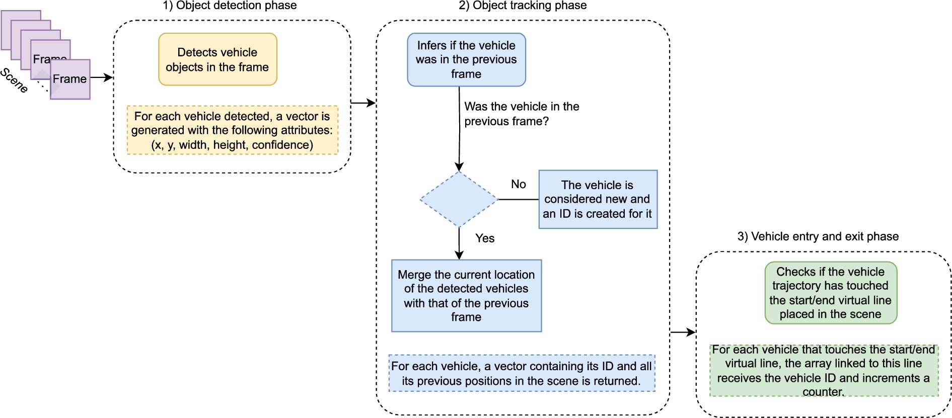
Overview of the proposed pipeline, comprising the vehicle detection, vehicle tracking, and origin-destination identification steps.

Roughly speaking, our pipeline receives a sequence of frames as input and processes each of them sequentially. The first phase is the object detection one (Section 3.2), which detects the vehicles on the frame using a fine-tuned YOLOv4 network [31]. The network is fine-tuned using the UAVDT dataset, as described in Section 3.1. Once a vehicle is detected, it is time for the object tracking phase (Section 3.3), where the positions of a vehicle within subsequent frames are used to form its trajectory. This step is performed using the tracking method proposed in [6]. Finally, the origins and destinations identification phase (Section 3.4) is responsible for detecting the entrance and exit points of each trajectory in order to allow summarizing the number of vehicles on each origin-destination pair within the intersection.

3.1. Dataset

In order to train and test our pipeline, we first had to search a dataset featuring traffic footage with aerial angulation and appropriately annotated vehicles. Meeting these requirements provide sufficient conditions to perform object detection and tracking tasks using CNN architectures.

We consider the UAVDT dataset [10]. The UAVDT dataset features traffic scenes with diverse heights (i.e., low, medium, high) and angulations (i.e., front, side, and bird). This dataset includes 50 different traffic scenes, totaling over 80,000 frames. However, in order to ensure that the whole intersection is captured in the scenes, we selected only a subset of scenes that are high enough to enable all incoming and outcoming lanes to be observed. This includes scenes with front or side views with at least medium altitude as well as bird view at any altitude. The final list of scenes is presented in Table 1. These scenes are essential to train the vehicle detector method, which we describe in detail in the next section.

Table 1
Subset of UAVDT dataset scenes used in our work for training and testing

Name Frames View Altitude Car Truck Bus Total vehicles Unique vehicles Type

M0101 407 Front+Side Medium 5156 188 70 5414 20 Train

M0210 583 Bird Medium 4725 1796 0 6521 33 Train

M0402 410 Side Medium 10210 0 0 10210 45 Train

M0601 372 Front+Side High 9908 150 365 10423 51 Train

M0606 1374 Front+Side Medium 17071 224 459 17754 96 Train

M0701 1308 Bird High 90563 2472 1008 94043 182 Train

M0702 777 Bird Medium 42042 386 3699 46127 94 Train

M0703 683 Bird Low 15235 643 628 16506 89 Train

M0801 298 Bird Low 3832 108 207 4147 24 Train

M1201 1197 Front+Side Medium 23080 4188 0 27268 59 Train

M0403 514 Front+Side Medium 31403 0 0 31403 99 Test

M0603 2035 Bird Medium 41478 1748 1500 44726 71 Test

Name	Frames	View	Altitude	Car	Truck	Bus	Total vehicles	Unique vehicles	Type
M0101	407	Front+Side	Medium	5156	188	70	5414	20	Train
M0210	583	Bird	Medium	4725	1796	0	6521	33	Train
M0402	410	Side	Medium	10210	0	0	10210	45	Train
M0601	372	Front+Side	High	9908	150	365	10423	51	Train
M0606	1374	Front+Side	Medium	17071	224	459	17754	96	Train
M0701	1308	Bird	High	90563	2472	1008	94043	182	Train
M0702	777	Bird	Medium	42042	386	3699	46127	94	Train
M0703	683	Bird	Low	15235	643	628	16506	89	Train
M0801	298	Bird	Low	3832	108	207	4147	24	Train
M1201	1197	Front+Side	Medium	23080	4188	0	27268	59	Train
M0403	514	Front+Side	Medium	31403	0	0	31403	99	Test
M0603	2035	Bird	Medium	41478	1748	1500	44726	71	Test

3.2. Object detection phase

At this stage of the pipeline, the main objective is to feed the frames provided by the dataset as input to the detector and identify the vehicles in the scene. The detector takes the input data and produces bounding boxes around the vehicles present in the scene, thus providing their locations.

In order to perform object detection, we employed the YOLOv4 network [31], which is considered the state-of-the-art architecture for real-time object detection. The YOLOv4 network was pre-trained with the COCO dataset. However, for the particular case of traffic scenes, this was not enough to yield satisfactory performance. To this end, we fine-tuned the YOLOv4 network using the UAVDT dataset.

We started with the Darknet implementation of YOLOv4.2

²
Available at https://github.com/AlexeyAB/darknet.

The loaded model had its first 136 layers frozen, while the remaining layers were unfrozen for fine-tuning. In this way, we aimed to accelerate the learning process while preserving the knowledge already acquired by the pre-trained model.

We further customized the input shape of the network to $832 \times 832$ pixels (the original network had an input of $512 \times 512$ pixels) to improve the performance of the network on distant scenes. The batch size and number of subdivisions were both set to 64. The number of channels was set to 3. The saturation and exposure values were both set to 1.5. The momentum value was set to 0.949, weight decay to 0.0005, learning rate to 0.001, and max batches to 6000 samples (the original network uses 2000 samples) in order to take into account the RAM limitations of our setup. Figure 2 illustrates the output of this phase. Our model was trained using Google Colab Pro, featuring a NVIDIA Tesla P100 GPU, providing significant computing power to our training process. The model was trained for a period of 30627 seconds (approximately 9 hours) and has an average inference cost of 0.07 seconds per frame.

Fig. 2.

Output of the vehicle detection phase based on a frame from the M0603 scene.

3.3. Object tracking phase

In the object tracking phase, each vehicle detected in the previous phase is tracked throughout a sequence of frames in order to enable the identification of its trajectory. This step is essential to enable the interpretation of the origins of destinations of the vehicles, as performed by the phase described in the next section.

We highlight that, although the object detection phase is the one responsible for identifying the vehicles, it is not able to tell whether an object appearing in subsequent frames represent the same vehicle. This is precisely the objective of the tracking phase, which needs to compare the position of vehicles in subsequent frames in order to have a unique correspondence.

To perform the task at hand, we utilized the tracker proposed in [6]. This method operates under the assumption that the detector produces a single detection per frame for each vehicle to be tracked. Essentially, for a given vehicle, the distance between its positions in consecutive frames must be either minimal or non-existent. Additionally, the method relies on the bounding boxes representing the vehicle in two successive frames having a substantial overlap, as measured by the Intersect Over Union (IoU) metric. We set the threshold for the IoU metric at 50%, meaning that to be considered the same object, the previous and current bounding boxes must have at least a 50% overlap.

Fig. 3.

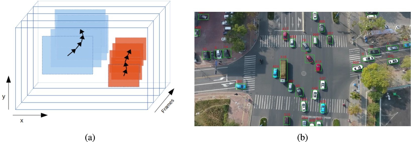
Object tracking phase, where (a) shows a sketch of the method proposed by [6], and (b) presents the output of the tracking phase based on a frame from the M0603 scene.

Figure 3a illustrates how the tracking technique works. In the figure, two objects are shown along a sequence of four frames. Each object is delimited by a bounding box and the arrow denotes its direction. Position are represented as x and y coordinates. As seen, for any object, the bounding boxes on subsequent frames present a high overlap. Building upon that observation, the trajectory of an object can be inferred by observing the position of its bounding box along frames.

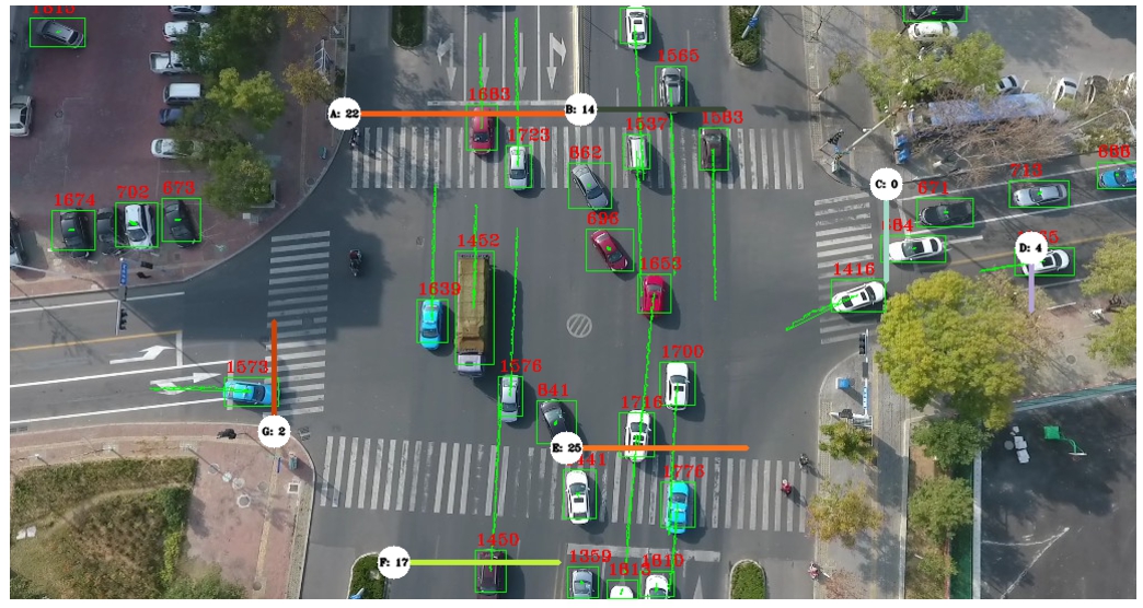
In this sense, after receiving the vehicle detection coordinates, the tracking algorithm starts its verification to infer whether the vehicle is new on the scene or not. If the vehicle is new, an ID is assigned to it. Otherwise, the newly perceived coordinates are stored in an array containing all coordinates previously detected for that particular vehicle. Figure 3b presents the result of the tracking method, where an ID is assigned to each vehicle identified in the previous stage.

3.4. Origin and destination identification

At this stage of the pipeline, the objective is to detect the points where a vehicle enters and exits the intersection. The idea is that, by detecting such points, one can infer the origin and destination of each vehicle. Recall that, for RL-based traffic light control, this information is of uttermost importance, as it allows the agent to properly model the flow of vehicles and make its decisions [23]. To this end, we define virtual lines in the frames to represent the entrance and exit points of the intersection, where each virtual line is composed of a pair of x and y coordinates. The sequence of steps of this phase are depicted in Fig. 4a.

Fig. 4.

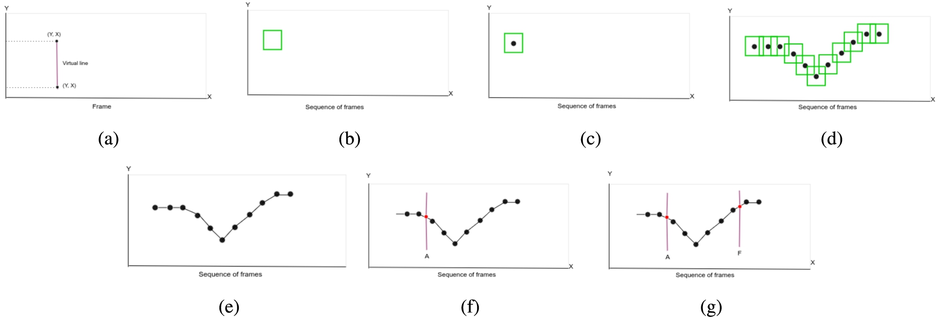
Origin and destination identification phase: (a) shows how the virtual lines are positioned in the scene; (b) illustrates the detection of a single vehicle in a single frame, and (c) its center; (d) presents the same vehicle being detected along multiple frames and their corresponding detection centers (e) shows the detection centers being joined by a line, thus representing a trajectory; (f) represents the moment that the trajectory touches the virtual line A; (g) illustrates the moment that the trajectory touches virtual line F. The tracking shown in (d) makes use of an IoU threshold lower than the one described in Section 3.3. This was done only for illustration purposes, in order avoid too close frames and thus enhance presentation.

In order to enable the identification of origins and destinations, virtual lines are placed at the entrances and exits of the intersections. Then, through the data provided by the tracking phase, it is possible to discover the entire trajectory of the vehicle along the scene based on the returned array of coordinates. For each coordinate, its center is calculated to generate the trajectory, as depicted in Fig. 4d. In this way, the trajectory is a set of centroids obtained from the array of coordinates, as seen in Fig. 4e.

To be able to know where a vehicle entered and exited the intersection, we calculate the intersection between the vehicle’s trajectory and the annotated virtual line, as shown in Figs 4f and 4g. If the intersection is positive, we store the vehicle ID in an array associated with the respective straight segment. In addition, we increment a counter that shows how many vehicles have passed through that line.

Fig. 5.

Identification of the origins and destinations of the vehicles based on frames from the M0603 (Fig. 6a) and M0403 (Fig. 6b) scenes.

In Fig. 5, we can observe the operation of the pipeline. In the figure, once vehicles and their trajectories are detected, it is possible to compute through which entrance and exit lines each vehicle goes through. Such information can then be used to count the number of vehicles on each origin and destination pair within the given intersection.

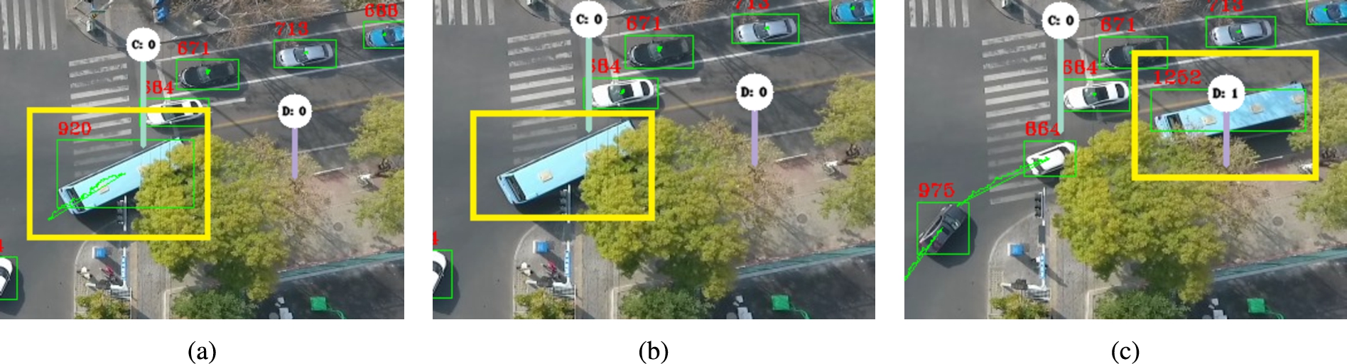
As mentioned in Section 3.3, the object detection phase is not able to distinguish between object instances; it only tells where each object is placed at the scene. Our tracking algorithm is then responsible for discerning between them by a certain degree of confidence. Unfortunately, there are cases in which we lost track in the middle of the experiment. For instance, consider the bus tracked in Fig. 6a with id 920 (the one turning right). In the next frame (Fig. 6b), when the bus passes beneath the tree, the detector fails to detect the given bus. Once the bus crosses the tree (Fig. 6c), the detector is again able to detect the bus. However, as the connection with the previous frames was lost, our algorithm assigns it a new id, namely 1520, and after that the bus crosses an end-point. So, as shown in this example, the object with id 1252 seems to only crosses an end-point, but without ever crossing any starting point.

In order for a vehicle’s track to be counted as finished, it must cross both the start point and end point. If the detector loses track of a vehicle in the middle of its journey, a new ID is assigned and its track begins again. This can occur multiple times for the same vehicle, resulting in its ID being reassigned and its track being restarted. To address this issue, our approach is straightforward: we identify all tracks that have crossed the end point but not the start point (a.k.a output tracks) and attempt to match them with tracks that have crossed the start point but not the end point (a.k.a. input tracks). Our aim is to find the shortest distance between the last frame of the input track and the first frame of the output track, thereby determining if the two tracks correspond to the same vehicle.

In the example shown in Fig. 7, the detector loses track of a bus multiple times, resulting in the creation of several tracks for the same vehicle, including both input and output tracks. After the simulation is completed, our algorithm attempts to match each output track with an input track by using the shortest distance criteria between the last frame of the input track and the first frame of the output track. In this particular case, the algorithm matches output track 1272 with input track 748, combining them both into a single track with ID 748, thus establishing an origin-destination pair. It is worth noting that track 1182, shown in Fig. 7d, is neither an input track (as it has not crossed a start point) nor an output track (as it has not crossed an end point), and therefore it is not included in the matching algorithm.

Fig. 6.

Tracker losing identification on vehicle. As the bus from Fig. 6a passes beneath the tree, the tracker loses its track, as shown in Fig. 6b. Later, in Fig. 6c, when the bus became once again detectable, the tracker associates that object as a new one; thus, assigning it a new id.

Fig. 7.

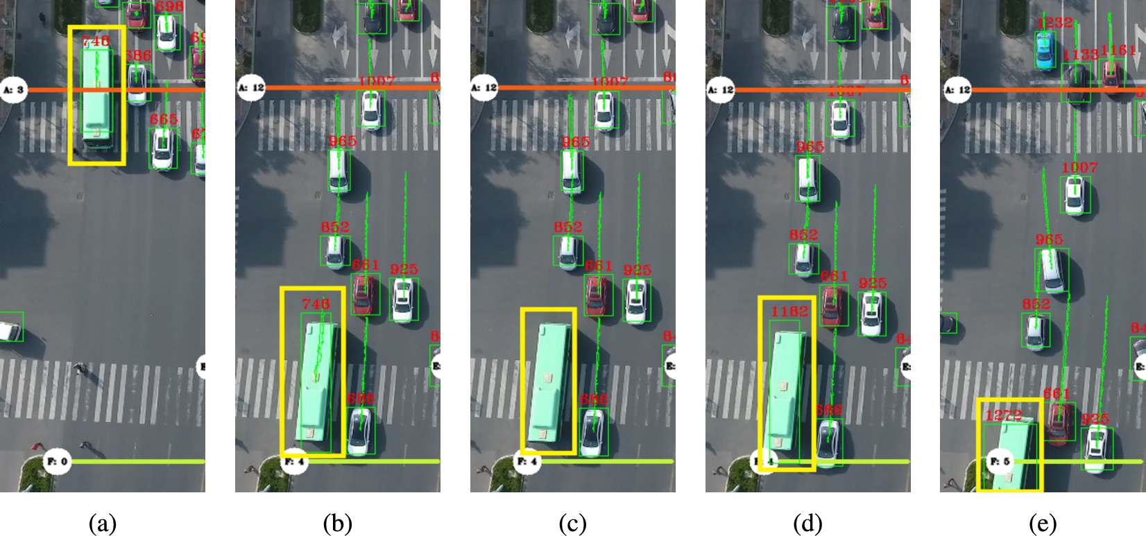
This example demonstrates the method described in Section 3.4. In Fig. 7a, the center of the bus’ bounding box crosses imaginary line A, marking this track (known as track 748) as a new input track. The detector continues to track the bus without issue until Fig. 7b, where it fails to detect the bus in the next frame (Fig. 7c), resulting in the loss of track 748. In Fig. 7d, the detector detects the bus again, but assigns it a new track (track 1182) since track 748 was lost. As mentioned in Section 3.4, this loss of detection can occur multiple times for the same object, as is evident in Fig. 7e, where the center of the bus’ bounding box crosses imaginary line F with a track ID of 1272 (indicating that the detector failed to detect the bus again). Track 1272 is an output track. After completing the detection run, our algorithm matches the closest pairs between input and output tracks, combining them to create a single track. In this case, tracks 748 and 1272 are matched, resulting in a single track with an ID of 748 (using the ID of the input track).

4. Experimental evaluation

The experiments were conducted to evaluate the performance of each phase of the pipeline and the complete pipeline. The evaluation methodology is described in Section 4.1, and the results are discussed in Section 4.2.

4.1. Methodology

In order to test our pipeline, we selected the scenes M0403 and M0603 from the UAVDT dataset. To evaluate the pipeline, we adopted two complementary strategies. The first one is to evaluate the pipeline’s task, which is multi-object tracking. Measuring the performance of multi-object trackers requires some care. Although a variety of assessment metrics have been proposed in the literature [24], there has yet to be a general consensus on the best set of metrics to use. In this sense, we decided to employ the following metrics. In the list, the arrows in parentheses indicate whether each metric should be maximized (↑) or minimized (↓).

IDF1 (↑): global min-cost F1 score.

IDP (↑): global min-cost precision.

IDR (↑): global min-cost recall.

Recall (↑): number of detections over number of objects

Precision (↑): number of detected objects over sum of detected and false positives.

FP (↓): total number of false positives.

FN (↓): total number of misses.

IDs (↓): total number of track switches.

MOTA (↑): multiple object tracker accuracy.

MOTP (↑): multiple object tracker precision.

IDF1 is a metric that combines precision and recall to evaluate the performance of multi-object tracking algorithms. It is based on optimal assignment between ground truth objects and detected objects. The IDP and IDR metrics are calculated based on optimal assignment between ground truth objects and detected objects. The recall metric assesses the algorithm’s ability to detect all objects in the scene, while precision measures its ability to avoid false positives. False positives refer to objects falsely detected as present, while false negatives (FN) refer to objects present in the scene but not detected by the algorithm. The IDs metric provides an indication of tracking stability, with a lower value indicating better tracking. MOTA calculates the percentage of errors made by the algorithm in tracking all objects, while MOTP measures tracking accuracy in terms of object positions.

The strategy to evaluate the complete pipeline, on the other hand, requires metric able to compare the number of vehicles on each origin-destination pair as output by our pipeline in comparison to the ground truth counting. To this end, we propose a new metric called OD Counting Error, as shown below: $\begin{matrix} (1) & OD Counting Error = \frac{1}{GT} \sum_{i = 0}^{n} | {Detection}_{i} - {GT}_{i} |, \end{matrix}$ where GT is the total number of vehicles that completed their routes, n represents the number of OD pairs in the scene (which in this case is the same as the number of routes), ${Detection}_{i}$ and ${GT}_{i}$ denote the number of vehicles from OD pair i that completed their routes as detected by our pipeline and represented as ground truth, respectively. An intuitive description of the newly proposed metric is provided in Fig. 8, where an illustrative traffic intersection with 20 vehicles is explained and the resulting $OD Counting Error$ is computed. This metric is employed to assess our pipaline in the next section by means of Tables 4 and 5.

Fig. 8.

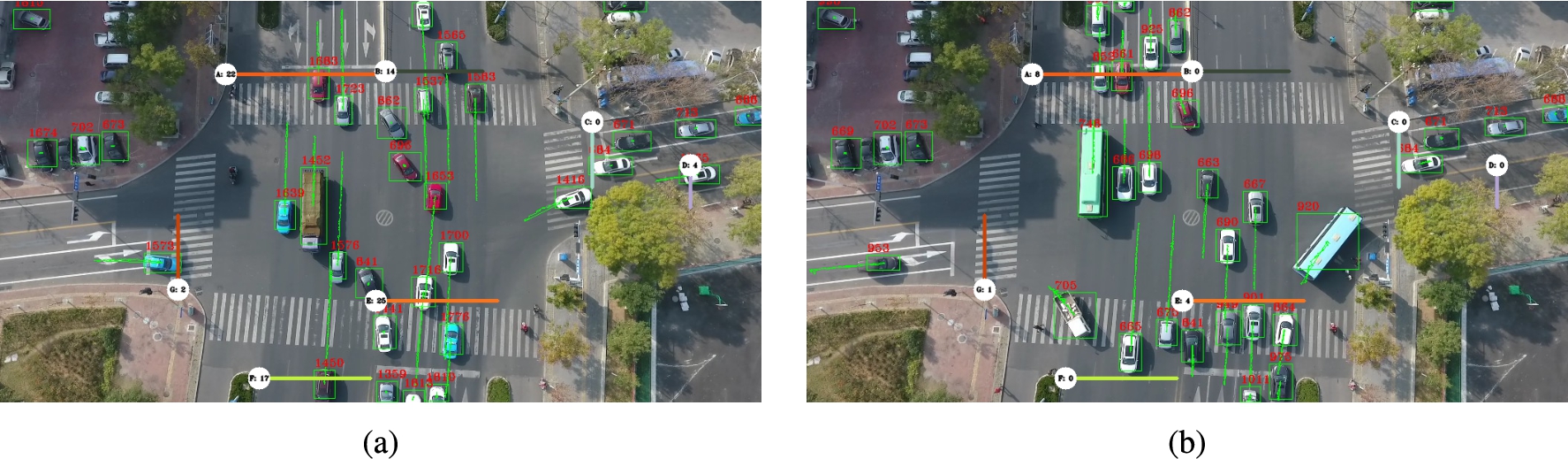
An example of the newly proposed metric (Eq.(1)) can be illustrated as follows. Consider two OD pairs (AC and AB). Figure (a) shows the ground truth, indicating that ${GT}_{AB} = 10$ , ${GT}_{AC} = 10$ , and $GT = 20$ . Figure (b) shows our detection results, where we intentionally made a mistake in identifying the AC pair, resulting in ${Detection}_{AB} = 10$ and ${Detection}_{AC} = 9$ . When the OD Counting Error metric is computed using Eq. (1), we obtain a value of $OD Counting Error = 0.05$ , indicating that we lost tracking of 5% of the OD pairs.

In order to better assess the performance of our approach, we adopted [37] as a baseline method for object detection and tracking, which we consider to be the state of the art in the context of traffic. As for the origin-destination identification part, we include no comparison given the lack of works on the topic.

Our experiments were executed in two different environments. The object detector was trained using Google Colab Pro, featuring a NVIDIA Tesla P100 GPU. The remaining experiments, in turn, were performed on a standard computer with Intel Core i7 CPU with 16GB of RAM and a NVIDIA GeForce RTX 2060 GPU.

Table 2

Results for the vehicle detection and vehicle tracking methods. Arrows denote whether metrics should be maximized (↑) or minimized (↓). Best results are highlighted in bold

Metrics	M0603	M0403	Average	State-of-art [37]
Frames	2035	514	2549	–
IDF1 ↑	82.5%	90.6%	85.7%	62.6%
IDP ↑	72.4%	86.1%	77.5%	76.00%
IDR ↑	95.9%	95.5%	95.8%	58.00%
Recall ↑	98.4%	97.8%	98.2%	–
Precision ↑	74.3%	88.3%	79.5%	–
FP ↓	15241	4087	19328	–
FN ↓	726	677	1403	–
IDs ↓	57	45	102	–
MOTA ↑	64.2%	84.7%	72.6%	43.1%
MOTP ↑	74.6%	74.1%	74.4%	78.5%

4.2. Results

We start the results section by analyzing the performance of our pipeline in its first two phases, the vehicle detector and the vehicle tracker. Table 2 presents the results obtained by our method and the baseline for the M0603 and M0403 scenes of the UAVDT dataset. As seen, the average results obtained by our pipeline outperform the current state-of-the-art approach by a good margin for most metrics. These results indicate that our pipeline is able to properly detect and track vehicles. This was made possible because we used a fine-tuned version of the YOLOv4 network, which yielded superior results than those obtained by the siamese network used in [37]. Moreover, since the our method yields better detections, the tracking phase ends up outperforming [37] as well.

The detector achieved a precision of 79.5%. This result directly influence the accuracy of the tracker, which ended up with an MOTP 74.4%. In order to improve the accuracy of the detector, it is necessary to train the model with more instances of the truck and bus classes, whose number was not sufficient in the UAVDT dataset. Throughout the experiments we observed that these specific classes end up failing more than cars. In addition, the use bird view images hinders the identification of smaller objects in the image. To improve this aspect, one could increase the size of the network at the time of training, which could enhance the accuracy at the cost of increasing the complexity of the object detection network.

Table 3 presents the results related to the number of vehicles that passed through each virtual line drawn in the scenes. Observe that the number of virtual lines is seven and nine for the M0603 and M0403 scenes, respectively. Results are compared to the annotated ground truth values. As seen, our method correctly detected all cases in the first scene and mistakenly detected only 3.38% of the cases in the second scene. We remark that the errors occurred because the detector failed to identify these vehicles. These errors could be reduced by improving the accuracy of the detector.

Table 3
Results for the number of vehicles passing through each virtual line for scenes M0403 and M0603

Virtual line M0603 M0403

GT Detections Error (N) GT Detections Error (N)

A 24 24 0 28 27 1

B 26 26 0 5 2 3

C 0 0 0 3 3 0

D 5 5 0 8 8 0

E 36 36 0 22 22 0

F 25 25 0 3 3 0

G 3 3 0 3 3 0

H − − – 5 5 0

I − − – 9 9 0

Virtual line	M0603	M0403
A	24	24	0	28	27	1
B	26	26	0	5	2	3
C	0	0	0	3	3	0
D	5	5	0	8	8	0
E	36	36	0	22	22	0
F	25	25	0	3	3	0
G	3	3	0	3	3	0
H	−	−	–	5	5	0
I	−	−	–	9	9	0

Table 4

Origin-destination identification results for the M0603 scene

OD Pair	GT	Detections	OD Error by Route	–
A to F	22	22	0	–
E to B	26	26	0	–
E to D	5	4	1	–
G to F	3	3	0	–
OD Error % ↓	56	55	1	1.78%

Table 4 presents the overall results of our pipeline on the M0603 scene by means of the OD Error metric. Recall that this metric shows for how many vehicles the pipeline failed to identify their complete trajectories. As seen in the table, our pipeline missed a single vehicle, which goes from E to D. In that case, the error happened because part of the scene is occluded, which prevented the detector from detecting the vehicles on that part of the scene. This situation is illustrated in Fig. 6, where the vehicle with ID 920 becomes undetectable when passing close to a tree and then becomes detectable again, thus receiving a new ID (namely 1252). In addiction to that, the detector was not well trained to deal with different classes of vehicles (such as buses). That fact increases the difficulty of finding a continuous track, as well as its origin and destination.

Table 5

Origin-destination identification results for the M0403 scene

OD Pair	GT	Detections	OD Error by Route	–
A to D	5	5	0	–
A to E	12	12	0	–
C to B	3	2	1	–
F to G	3	3	0	–
OD Error % ↓	23	22	1	4.35%

Finally, Table 5 presents the overall results of our pipeline on the M0403 scene by means of the OD Error metric. As seen, only a single vehicle was not properly identified, which represents a percentage error of 4.35% in the identification of the complete trajectory of the vehicles. In this scene, no occlusion points exist. However, the error also happened due to a failure in the detector. After the vehicle started its trajectory entering C, the detector failed, as such the vehicle ended up receiving a new ID before ending its trajectory.

5. Conclusions

This paper introduced a comprehensive pipeline for accurately extracting vehicle origins and destinations in traffic intersections. To achieve this, we first developed a customized YOLOv4 neural network that is fine-tuned using the UAVDT dataset and can detect vehicles with larger input images of size 832 x 832. We also proposed a vehicle tracking algorithm that can identify the trajectory of a vehicle across multiple frames, enabling accurate analysis of their movements. Finally, we presented an innovative algorithm that analyzes vehicle trajectories and extracts the number of vehicles in each origin and destination lane of the intersection. Together, these contributions enabled us to accurately recognize vehicles, their trajectories, and their origin and destinations in traffic intersections, providing essential information for enabling reinforcement learning agents to control traffic lights and address other traffic problems. This information can be used to improve traffic flow, reduce congestion, and enhance safety at intersections, among other potential applications.

In general, the pipeline obtained promising results, achieving an average error rate as low as 3.065% in terms of origins and destinations identification. However, some aspects of the pipeline presented less impressive results when facing occlusions or even when facing trajectory interruptions. We achieved an average precision of 79.5%, which detracted from the tracker accuracy, which reached 74.4%.

As part of our future work, we aim to enhance the accuracy of our model by training it on a larger dataset to increase its precision and thereby improve the tracker’s accuracy. We also plan to extend our model to handle multi-camera setups, which could potentially overcome occlusion-related challenges. Additionally, we intend to incorporate techniques from the literature, such as those proposed in [16], to improve our tracking algorithm’s ability to analyze situations where vehicles may appear or disappear due to detection loss. These changes would be a significant step towards deploying our pipeline in real-world scenarios.

Moreover, we are interested in exploring the use of the latest object detection architectures, such as Vision Transformers [9] and SWIN Transformers [22], to enhance the accuracy of vehicle detection. This direction of future work could further improve the performance of our pipeline and potentially achieve even better results in real-world applications.

Footnotes

Acknowledgements

We thank the anonymous reviewers for their valuable feedback. This research was partially supported by Coordenação de Aperfeiçoamento de Pessoal de Nível Superior – Brasil (CAPES) – Finance Code 001, Conselho Nacional de Desenvolvimento Científico e Tecnológico – CNPq (grants 306395/2017-7 and 314042/2021-0), Fundação de Amparo à Pesquisa do Estado do Rio Grande do Sul – FAPERGS (grants 17/2551-0001197-0, 19/2551-0001277-2, and 19/2551-0001334-5), and Fundação de Amparo à Pesquisa do Estado de São Paulo – FAPESP (grant 2020/05165-1).

References

M.H.

Ali ,

Kurokawa and

Shafie , Autonomous road surveillance system: A proposed model for vehicle detection and traffic signal control, Procedia Computer Science19 (2013), 963–970. doi:10.1016/j.procs.2013.06.134.

Arinaldi ,

J.A.

Pradana and

A.A.

Gurusinga , Detection and classification of vehicles for traffic video analytics, Procedia Computer Science144 (2018), 259–268. doi:10.1016/j.procs.2018.10.527.

Arnott and

Small , The economics of traffic congestion, American scientist82(5) (1994), 446–455.

A.L.C.

Bazzan and

Klügl , Introduction to intelligent systems in traffic and transportation, Synthesis Lectures on Artificial Intelligence and Machine Learning7(3) (2013), 1–137. doi:10.1007/978-3-031-01565-6.

Bewley ,

Ge ,

Ott ,

Ramos and

Upcroft , Simple online and realtime tracking, in: 2016 IEEE International Conference on Image Processing (ICIP), IEEE, 2016, pp. 3464–3468. doi:10.1109/ICIP.2016.7533003.

Bochinski ,

Eiselein and

Sikora , High-speed tracking-by-detection without using image information, in: International Workshop on Traffic and Street Surveillance for Safety and Security at IEEE AVSS 2017, 2017.

Chintalacheruvu and

Muthukumar , Video based vehicle detection and its application in intelligent transportation systems, Journal of Transportation Technologies02(04) (2012), 305–314. doi:10.4236/jtts.2012.24033.

Dai ,

Song ,

Wang ,

Fang ,

Yun ,

Zhang and

Li , Video-based vehicle counting framework, IEEE Access7 (2019), 64460–64470. doi:10.1109/ACCESS.2019.2914254.

Dosovitskiy ,

Beyer ,

Kolesnikov ,

Weissenborn ,

Zhai ,

Unterthiner ,

Dehghani ,

Minderer ,

Heigold ,

Gelly et al., An image is worth 16x16 words: Transformers for image recognition at scale, 2020, arXiv preprint arXiv:2010.11929.

10.

Du ,

Qi ,

Yu ,

Yang ,

Duan ,

Li ,

Zhang ,

Huang and

Tian , The unmanned aerial vehicle benchmark: Object detection and tracking, 2018.

11.

V.A.

Fraga ,

Schreiber ,

Kunst ,

J.L.C.

Barbosa and

G.de.O.

Ramos , A machine learning pipeline for extracting decision-support features from traffic scenes, in: Proceedings of the 12th Workshop on Agents in Traffic and Transportation (ATT-2022),

A.L.C.

Bazzan ,

Dusparic ,

Lujak and

Vizzari , eds, Vol. 3173, Vienna, 2022, pp. 194–208.

12.

Girshick , Fast r-cnn, in: Proceedings of the IEEE International Conference on Computer Vision, 2015, pp. 1440–1448.

13.

Girshick ,

Donahue ,

Darrell and

Malik , Rich feature hierarchies for accurate object detection and semantic segmentation, in: Proceedings of the IEEE Conference on Computer Vision and Pattern Recognition, 2014, pp. 580–587.

14.

S.-C.

Huang and

B.-H.

Chen , Highly accurate moving object detection in variable bit rate video-based traffic monitoring systems, IEEE Transactions on Neural Networks and Learning Systems24(12) (2013), 1920–1931. doi:10.1109/tnnls.2013.2270314.

15.

Iwasaki ,

Misumi and

Nakamiya , Robust vehicle detection under various environmental conditions using an infrared thermal camera and its application to road traffic flow monitoring, Sensors13(6) (2013), 7756–7773. doi:10.3390/s130607756.

16.

S.D.

Khan ,

Bandini ,

Basalamah and

Vizzari , Analyzing crowd behavior in naturalistic conditions: Identifying sources and sinks and characterizing main flows, Neurocomputing177 (2016), 543–563. doi:10.1016/j.neucom.2015.11.049.

17.

Law and

Deng , Cornernet: Detecting objects as paired keypoints, in: Proceedings of the European Conference on Computer Vision (ECCV), 2018, pp. 734–750.

18.

Law ,

Teng ,

Russakovsky and

Deng , Cornernet-lite: Efficient keypoint based object detection, 2019, arXiv preprint arXiv:1904.08900.

19.

T.-Y.

Lin ,

Maire ,

Belongie ,

Hays ,

Perona ,

Ramanan ,

Dollár and

C.L.

Zitnick , Microsoft coco: Common objects in context, in: European Conference on Computer Vision, Springer, 2014, pp. 740–755.

20.

Liu ,

Zeng and

Jiang , A video-based real-time adaptive vehicle-counting system for urban roads, PloS one12(11) (2017), e0186098. doi:10.1371/journal.pone.0186098.

21.

Liu ,

Anguelov ,

Erhan ,

Szegedy ,

Reed ,

C.-Y.

Fu and

A.C.

Berg , Ssd: Single shot multibox detector, in: European Conference on Computer Vision, Springer, 2016, pp. 21–37.

22.

Liu ,

Lin ,

Cao ,

Hu ,

Wei ,

Zhang ,

Lin and

Guo , Swin transformer: Hierarchical vision transformer using shifted windows, in: Proceedings of the IEEE/CVF International Conference on Computer Vision (ICCV), 2021, pp. 10012–10022.

23.

Mannion ,

Duggan and

Howley , An experimental review of reinforcement learning algorithms for adaptive traffic signal control, in: Autonomic Road Transport Support Systems, 2016, pp. 47–66. doi:10.1007/978-3-319-25808-9_4.

24.

Milan ,

Leal-Taixe ,

Reid ,

Roth and

Schindler , MOT16: A Benchmark for Multi-Object Tracking, 2016.

25.

Mudoi and

P.A.

Kashyap , Vision based data extraction of vehicles in traffic, in: 2014 International Conference on Signal Processing and Integrated Networks (SPIN), IEEE, 2014, pp. 202–208. doi:10.1109/SPIN.2014.6776948.

26.

Ren ,

He ,

Girshick and

Sun , Faster r-cnn: Towards real-time object detection with region proposal networks, Advances in neural information processing systems28 (2015), 91–99.

27.

Schreiber ,

L.N.

Alegre ,

A.L.C.

Bazzan and

G.de.O.

Ramos , On the explainability and expressiveness of function approximation methods in RL-based traffic signal control, in: 2022 International Joint Conference on Neural Networks (IJCNN), IEEE, Padova, Italy, 2022. doi:10.1109/IJCNN55064.2022.9892422.

28.

Sochor ,

Špaňhel and

Herout , Boxcars: Improving fine-grained recognition of vehicles using 3-d bounding boxes in traffic surveillance, IEEE transactions on intelligent transportation systems20(1) (2018), 97–108. doi:10.1109/TITS.2018.2799228.

29.

Tang ,

Wu ,

Jin ,

Zou and

Li , Multi-modal metric learning for vehicle re-identification in traffic surveillance environment, in: 2017 IEEE International Conference on Image Processing (ICIP), IEEE, 2017. doi:10.1109/icip.2017.8296683.

30.

Tang ,

Y.C.

Xu and

C.Z.

Zhang , Robust vehicle detection based on cascade classifier in traffic surveillance system, The Open Automation and Control Systems Journal6(1) (2014), 349–354. doi:10.2174/1874444301406010349.

31.

C.-Y.

Wang ,

Bochkovskiy and

H.-Y.M.

Liao , Scaled-YOLOv4: Scaling Cross Stage Partial Network, 2021.

32.

Wang ,

Simeonova and

Shahbazi , Orientation-and scale-invariant multi-vehicle detection and tracking from unmanned aerial videos, Remote Sensing11(18) (2019), 2155. doi:10.3390/rs11182155.

33.

Wang ,

Xiao ,

Xiao and

Li , Fine-grained vehicle recognition in traffic surveillance, in: Pacific Rim Conference on Multimedia, Springer, 2016, pp. 285–295.

34.

Wei ,

Zheng ,

V.V.

Gayah and

Li , A Survey on Traffic Signal Control Methods, 2019, arXiv:1904.08117.

35.

Wojke ,

Bewley and

Paulus , Simple online and realtime tracking with a deep association metric, in: 2017 IEEE International Conference on Image Processing (ICIP), IEEE, 2017, pp. 3645–3649. doi:10.1109/ICIP.2017.8296962.

36.

Yang and

Qu , Real-time vehicle detection and counting in complex traffic scenes using background subtraction model with low-rank decomposition, IET Intelligent Transport Systems12(1) (2017), 75–85. doi:10.1049/iet-its.2017.0047.

37.

Yu ,

Li ,

Zhang ,

Huang ,

Du ,

Tian and

Sebe , The unmanned aerial vehicle benchmark: Object detection, tracking and baseline, International Journal of Computer Vision128(5) (2020), 1141–1159. doi:10.1007/s11263-019-01266-1.

38.

Zear ,

Singh and

Singh , Intelligent transport system: A progressive review, Indian Journal of Science and Technology9 (2016). doi:10.17485/ijst/2016/v9i32/100713.

39.

Zhang ,

F.-Y.

Wang ,

W.-H.

Lin ,

Xu and

Chen , Data-driven intelligent transportation systems: A survey, IEEE Transactions on Intelligent Transportation Systems12(4) (2011), 1624–1639. doi:10.1109/TITS.2011.2158001.

A machine learning pipeline for extracting decision-support features from traffic scenes 1

Abstract

Keywords

1. Introduction

2. Related work

3. Proposed pipeline

2 Available at https://github.com/AlexeyAB/darknet.

4.1. Methodology

Footnotes

Acknowledgements

References

²
Available at https://github.com/AlexeyAB/darknet.