Automated detection of vehicles with anomalous trajectories in traffic surveillance videos

Abstract

Video feeds from traffic cameras can be useful for many purposes, the most critical of which are related to monitoring road safety. Vehicle trajectory is a key element in dangerous behavior and traffic accidents. In this respect, it is crucial to detect those anomalous vehicle trajectories, that is, trajectories that depart from usual paths. In this work, a model is proposed to automatically address that by using video sequences from traffic cameras. The proposal detects vehicles frame by frame, tracks their trajectories across frames, estimates velocity vectors, and compares them to velocity vectors from other spatially adjacent trajectories. From the comparison of velocity vectors, trajectories that are very different (anomalous) from neighboring trajectories can be detected. In practical terms, this strategy can detect vehicles in wrong-way trajectories. Some components of the model are off-the-shelf, such as the detection provided by recent deep learning approaches; however, several different options are considered and analyzed for vehicle tracking. The performance of the system has been tested with a wide range of real and synthetic traffic videos.

Keywords

Anomaly detection video surveillance object tracking object detection deep learning

1. Introduction

There has been a historic increase in video surveillance cameras in public and private places. This trend has resulted in a wide variety of research studies about automated systems for object detection to monitor different activities by recognizing the events that occur in the observed scene [1]. These systems play an important role in modern computer vision tasks such as autonomous driving [2], pedestrian identification [3, 4] image captioning [5, 6], object tracking [7, 8] ship detection [9, 10], face recognition [11, 12], traffic control [13, 14] action recognition [15, 16] environment surveillance [17, 18], video checking in sports [19, 20], building information [21, 22, 23], robotic disinfection [24], safety surveillance [25, 26] and many others. Deep Learning has been the main approach when dealing with images for the last decade. Beyond surveillance it is an approach also applied to other fields such as material analysis [27], earthquake detection [28], medical applications [29, 30] and recommendation systems [31].

This work focuses on vehicle detection, an important part of surveillance systems and intelligent transport systems. The widespread use of vehicles means that numerous incidents regarding traffic violations occur. These incidents can be seen as anomalies with respect to the usual traffic behavior and are typically a source of problems and dangers. Therefore the detection of anomalies in traffic surveillance such as traffic congestion, parking violations, and rash driving on the roads can be considered one of the most researched topics in vehicle detection [32].

However, the automated detection of vehicles that follow an unusual, wrong-way trajectory has not received much attention in the literature. Here a methodology to detect wrong-way vehicle trajectories is proposed. Its aim is to automatically spot potentially dangerous behavior. This information could be later passed on to a human operator so that the danger is further evaluated and cautionary measures can be taken. This model is capable of monitoring, frame by frame, the movement of the vehicles to identify vehicles that drive in an unusual way by using three basic steps: vehicle detection, vehicle tracking, and trajectory processing. Our proposal departs from the previous literature in several ways. Firstly, vehicle tracking is optimized by several enhancements in the assignment procedure of vehicle detections to trajectories. Also, tracking errors for pairs of nearby vehicles and large trucks are minimized by appropriate techniques. Finally, a robust anomaly measure is designed in order to effectively evaluate trajectories, and an anomaly criterion is proposed to ascertain whether a trajectory is actually anomalous.

For moving vehicle detection, a Convolutional Neural Network is used because it can perform end-to-end detection of objects without specific characteristics [33]. Then the set of detections computed by the network is filtered to execute the second step, vehicle tracking. In this stage, vehicles are tracked as they move around in a video using two popular object tracking algorithms, Simple Online Real Time tracking (SORT) and BYTE. These algorithms can make some tracking errors in specific situations so a custom tracking algorithm is proposed and compared with the previous ones. Once trajectories are detected they are processed, which is the third step. In this phase, the velocity vectors are estimated by comparing the difference in the position of the vehicle between consecutive image frames, and anomalies are detected by comparing the vehicle’s trajectories with the trajectories of its nearest neighbors using mean and median moduli of the differences among vector velocities.

As this method has many tunable parameters, a comprehensive survey was conducted, including the impact of adding techniques such as border correction and bounding box similarity. This fine-tuning process concludes in a suitable procedure for detecting anomalous trajectories.

To describe the above mentioned methodology in detail, the paper is arranged as follows. First, Section 2 summarizes the related work. Then, the methodology to solve the stated problem is described in detail in Section 3. After that, in Section 4, experimental results are provided to verify the performance of the proposed model. And finally, Section 5 outlines the conclusions.

2. Related work

There are many techniques proposed in the literature to detect on-road traffic. Object detection can be performed using either classical image processing techniques or deep learning networks. Today, deep learning object detection is a modern approach widely accepted by researchers, involving two main types of detectors: two-stage target detection algorithms and single-stage target detection algorithms. As a general algorithm for target detection, all the deep learning models can be applied to vehicle detection tasks. Two-stage detection algorithms divide the vehicle detection task into two stages: generating vehicle region proposals and finding vehicle targets from the region proposal. One-stage detection algorithms eliminate the operation of generating vehicle region proposals and unifies vehicle identification and detection into one network for processing.

An example of a traditional proposal can be found in [34], where it uses a foreground object detection method and a feature extractor to obtain the most significant features of the detected vehicles into several categories such as car, motorcycle, truck, or van. The same task is addressed by two-stage algorithms in [35, 36] and [37] where a Convolutional Neural Network (CNN) is used in the first two cases and a Faster Regional Convolutional Neural Network (Faster R-CNN) in the third one. The most representative one-stage detector is YOLO [38] (You Only Look Once) and [39] combines it with other traditional classifiers to create a real-time vehicle detector. In [40] a comprehensive review of existing Faster Region-based Convolutional Neural Network (Faster R-CNN) and YOLO-based vehicle detection and tracking methods are included so the interrelations between both methods can be highlighted.

After carrying out an assessment of the advances in the field of traffic video surveillance, it is interesting to notice that there are other relevant problems whose solution is related to the analysis and detection of vehicles along the road. This is the case of the detection of pollution levels of transport vehicles problem which has been addressed in [41, 42]. In these works, the object detection and classification process are based on a pre-trained Faster-RCNN model [43]. With that recognition and vehicle tracking, the system predicts the pollution of the selected area in real time. Another example can be found in [44], where a video measurement system for road traffic surveillance has been developed and applied to acoustic surveillance. This system includes a trained deep learning YOLOv2 object detection model and uses it to show the usefulness of Intelligent Transportation Systems (ITS) in the fight against citizens’ exposure to noise.

In terms of trajectory analysis, the problem has also been approached with classical algorithms before deep learning such as [45], which analyses vehicle trajectories using clustering algorithms; or [46] using single-class SVM clustering to allow trajectory classification with no a priori information on the distribution outliers. Modern approaches often rely on neural networks as [47], which trains a neural network model to detect pedestrian trajectory anomalies by comparing predicted and actual trajectories; in [13], authors propose a methodology to detect anomalous vehicle trajectories by applying YOLOv5 as a vehicle detection network; [48] uses multi-scale tracking and multiple similarity metrics to refine anomaly via backtracking after detecting vehicles using YOLO; [49] also uses YOLO, Non-Maximum-Suppression algorithm and DeepSort [50] to obtain trajectories prior to filter them; [51] implements a noisy network using deep deterministic policy gradients to deal with the tracking task and predict the trajectory result; [52] uses spatio-temporal autoencoder and sequence-to-sequence long short-term memory autoencoders in order to model spatial and temporal features in video to detect road accidents; [53] proposal is to use YOLO and KCF object tracking algorithm to get initial trajectories to later apply polynomial approximation and Ramer-Douglas-Peucker thinning to train agglomerative hierarchical clustering in order to classify into normal or anomaly trajectories; [54] implements NLP-inspired embedding to create vector representations for each vehicle trajectory in order to compute their similarities so a hierarchical clustering algorithm can be used to identified falsified trajectories; [55] extracts CNN features to perform two separate traffic analysis, the first one is based on the speed estimation using camera calibration and the second one based on detecting abnormal events using optical flow. However, there are also works nowadays using more classical approaches: [56] proposes a model to detect anomalies in vehicle trajectories by using federated learning based on support vector machines and isolation forests; [57] uses main flow direction vectors to cluster coarsely vehicle trajectories prior to apply K-means clustering algorithm to obtain fine classifications to distinguish outliers and then apply a hidden Markov model to obtain path pattern within each cluster.

Some works have also explicitly studied the problem of wrong-way vehicle detection. Early works used traditional image processing techniques such as background subtraction, and optical flow estimation [58, 59, 60], but these require very stable scene conditions and a relatively long training stage for each video sequence. More recent works make use of deep learning models to detect vehicles but usually require some degree of manual setup or assume a specific scene orientation to determine the natural direction of traffic flow in the scene [61, 62, 63]. In contrast, our approach is automatic, fully unsupervised, and does not require long training times for each specific scene. It is also dynamic: it does not look at whole trajectories post facto, but works frame by frame, using only past and present information at each frame to flag vehicles as following anomalous trajectories.

3. Methodology

To detect anomalous trajectories in sequences from traffic cameras, a model is proposed to monitor the movement of vehicles across the camera’s field of view frame by frame, with an architecture structured in three stages: vehicle detection, vehicle tracking and trajectory processing. a schematic view of the model is shown in Fig. 1.

Figure 1.

Schematic depiction of the proposed model.

Figure 1 shows a schematic of the proposed model: a video sequence from a traffic camera (a) is fed, frame by frame, to an object detector that outputs the vehicles’ bounding boxes (b). A tracking algorithm incrementally recovers vehicle trajectories (c, d) from the bounding boxes, possibly enhanced by various heuristics (not shown). At each frame $t+1$ , the velocity vector is the difference between positions at frames $t$ and $t+1$ (e), and this velocity vector is compared to the nearest velocity vectors from other trajectories (f), flagging the trajectory as anomalous if the vectors are different enough. See Section 3 for details.

3.1 Vehicle detection

Our proposed model starts with the application of a deep convolutional network for object detection to obtain tentative detections of vehicles. Let us note as $S$ the set of detections obtained by the object detection network $\mathcal{F}$ for a given input image $\mathbf{X}$ . Each detection $s_{i}$ contains an axis-aligned bounding box $\mathbf{w}_{i}$ , an object class label $q_{i}$ , and a confidence level $r_{i}$ :

$\displaystyle S=\mathcal{F}(\mathbf{X})$ (1) $\displaystyle S=\{s_{i}|i\in\{1,\ldots,N\}\}$ (2) $\displaystyle s_{i}=(\mathbf{w}_{i},q_{i},r_{i}),i\in\{1,\ldots,N\}$ (3) $\displaystyle\mathbf{w}_{i}=(a_{i},b_{i},c_{i},d_{i})$ (4)

where $N$ is the number of detections, $(a_{i},b_{i})\in\mathbb{\mathbb{R}}^{2}$ are the coordinates of the upper left corner of the $i$ -th detection within the image $\mathbf{X}$ , $(c_{i},d_{i})\in\mathbb{\mathbb{\mathbb{R}}}^{2}$ are the coordinates of the lower right corner of the $i$ -th detection within $\mathbf{X}$ , $q_{i}$ is the class label of the $i$ -th detection, and $r_{i}\in\mathbb{R}$ is the confidence level of the $i$ -th detection.

A minimum confidence level $r_{\min}$ is defined so that detections below that threshold are ignored. Moreover, the detections corresponding to non-vehicle classes are filtered out, and the object class is disregarded after that. As a result, the filtered set of detections is computed:

$\displaystyle S^{\prime}=\{s_{i}\in S|r_{i}\geqslant r_{\min},q_{i}\in V\}$ (5)

where $V$ is the set of vehicle classes.

The next step consists in passing the filtered set $S^{\prime}$ to the non-maximal-suppression algorithm to compute a further filtered set of detections $S^{\prime\prime}$ for the currently processed video frame, which is forwarded to the next stage, namely vehicle tracking.

3.2 Vehicle tracking

The second stage is object tracking: after objects have been detected and their bounding boxes defined at isolated image frames, the next challenge is to track the objects, associating bounding boxes across sequences of image frames conforming to the trajectories of each tracked object. Sophisticated tracking strategies are required when many objects move across the camera’s field of view.

For objects detected with bounding boxes, object tracking is frequently posed as a linear sum assignment problem (LSAP) [64] between the detections at frames $t+1$ and $t$ contained in the detection sets $S^{\prime\prime}_{t+1}$ and $S^{\prime\prime}_{t}$ , such that a cost $C_{ij}$ is specified for matching each pair of detections $s_{i}$ , $s_{j}\in S^{\prime\prime}$ , and there are off-the-shelf algorithms to arrive at an assignment between objects in frames $t$ and $t+1$ , minimizing the total cost. LSAP-based algorithms differ in the specification of the cost $C_{ij}$ and in pre and postprocessing steps, such as applying Kalman filters, or hierarchically classifying bounding boxes by confidence before matching them.

The performance of the pipeline is evaluated with two well-known, generic, LSAP-based object trackers, SORT [65] and BYTE [66], as well as a custom tracking algorithm. SORT and BYTE specify the assignment cost $C_{ij}$ as the intersection-over-union (also known as the Jaccard index [67]) between the bounding boxes. While specifying the cost in this way enables these object trackers to be robust, it can fail when objects with small apparent size move fast, and their bounding boxes in consecutive frames are very close but do not intersect. Because of this, in the custom tracking algorithm, the cost $C_{ij}$ of matching two detections $s_{i}$ , $s_{j}\in S^{\prime\prime}$ is specified as the Euclidean distance between the centers $\bm{\mu}_{i}$ , $\bm{\mu}_{j}$ of their associated bounding boxes:

$\displaystyle\bm{\mu}_{i}=\left(\frac{a_{i}+c_{i}}{2},\frac{b_{i}+d_{i}}{2}\right)$ $\displaystyle\bm{\mu}_{j}=\left(\frac{a_{j}+c_{j}}{2},\frac{b_{j}+d_{j}}{2}\right)$ (6) $\displaystyle C_{ij}=\|\bm{\mu}_{i}-\bm{\mu}_{j}\|$

When a vehicle detected in frame $t$ is not assigned a detection in frame $t+1$ , the model does not keep track of it in case it is detected later, given the apparent speeds of cars on traffic cameras. This often results in tracking errors. To compare the custom tracking algorithm with SORT and BYTE, they are also configured to not keep track of lost objects.

The performance of LSAP-based algorithms is adequate as long as objects movements between one frame and the next one are comparatively small, and the detection of the objects during the frame subsequence where they are visible is consistent. Videos acquired by traffic surveillance cameras used in this work usually fulfill the first condition. However, the second condition is not met even for object detectors with a very good mAP score for vehicles that appear small in the video. To address this limitation and enhance the performance of our custom tracking algorithm, we avoid making the assignments (i.e. matching bounding boxes for frames $t$ and $t+1$ as the same tracked vehicle across both time instants) that fulfill any of the following heuristics:

•

Given the two axis-aligned bounding boxes, the ratios of their sizes differs more than a given threshold in any of the two dimensions (horizontal or vertical). This aims to avoid false tracking events among vehicles of very different apparent sizes. Moreover, the system becomes more robust whenever the object detector fails and the bounding box estimations fluctuate from one frame to the next.

•

The distance between the centers of the bounding boxes in both frames is larger than a predefined threshold. The threshold is computed for each pair of bounding boxes relative to the smallest dimension of the bounding box at frame $t+1$ , rather than using a constant threshold. The aim of this procedure is to avoid wrong tracking events, where a vehicle is found at frame $t$ but not at the next frame $t+1$ while a third vehicle appearing at $t+1$ is wrongly assigned to the vehicle at time $t$ . Since object detection networks are more likely to fail in the detection of vehicles with small apparent sizes, this technique is particularly effective for distant vehicles in the analyzed scene. The technique can also be used for close vehicles with large apparent sizes, but it has to be slightly modified to take into account that such objects undergo large displacements that are not common for faraway vehicles. This is addressed by employing two distinct thresholds, one for vehicles with large bounding box sizes and another one for small sizes. Values for these thresholds have been found experimentally: if the length $d$ of the smallest side of the bounding box at $t+1$ is over 2.5% of the largest side of the image side, it is deemed to be part of the same trajectory as a bounding box at $t$ only if the distance between their centers is at most 1.25 times $d$ . If the bounding box is smaller (such vehicles can be described as having a small apparent size), the maximum distance between centers is 0.75 times $d$ .

Many tracking errors happen as a result of object detection errors and induce false, large one-frame displacements in trajectories, potentially confounding the anomaly detection procedure into generating false positives (see next subsection). In the case of small vehicles, such tracking errors can happen when two vehicles are close, only one is detected at frame $t$ , and only the other one is detected at frame $t+1$ . Large vehicles do not present this problem, but in the case of trucks, object detection can sometimes fail by detecting the cabin as a separate entity for an isolated frame. These kinds of object detection errors are difficult to solve even with domain-specific heuristics if the only input to the tracking algorithm is the set of bounding boxes. However, the subsequent tracking errors can be minimized, by noting that the contents of several bounding boxes identifying the same vehicle across several frames should be similar: if they are not similar enough, they should not be part of the same trajectory. There are complicating factors such as non-convex partial occlusions due to tree branches, but these are not as important for the purpose of anomalous trajectory detection.

This is a similar problem to vehicle re-identifica- tion [68], and can be solved with similar techniques. Concretely, to compute a similarity measure between the contents of the bounding boxes, the contents of each bounding box are resized (respecting the aspect ratio with letterboxing) to the input size of a standard deep classification network such as ResNet or VGG. This network is applied to the contents of the bounding box, and the feature vectors from one of its final layers are extracted. These feature vectors convey semantic information about the input image, and their distance can be used as a similarity measure for images. With this information, two bounding boxes are determined to be part of the same trajectory only if the similarity measure is below a given threshold.

To measure the distance between feature vectors, cosine similarity is used:

$\displaystyle d(u,v)=1-\frac{u\cdot v}{\|u\|_{2}\cdot\|v\|_{2}}$ (7)

This has practical advantages over Euclidean distance: the range of cosine similarity is clamped to the interval $[0\ldots 2]$ , while Euclidean distance is inherently dependent on the statistical distribution of the feature vectors. Calibration of the similarity threshold is necessary both for cosine similarity and Euclidean distance, but the calibration is easier for cosine similarity.

3.3 Trajectory processing

As a result of the vehicle tracking stage, vehicle trajectories are recovered across the camera’s field of view. The detection of anomalous maneuvers carried out by the vehicles can be done by comparing the trajectory of the offending vehicles to those of the vehicles in their vicinity. We propose a straightforward but effective procedure to accomplish this task which is based on measuring the difference between the velocity of the vehicle with respect to the velocities of its nearest neighbors. Here the velocity is taken as the difference in the position of the vehicle between consecutive image frames.

Next, a more detailed description of this procedure is given with the help of some mathematical notation. Let $\bm{\mu}_{i}(t)\in\mathbb{R}^{2}$ be the center of the bounding box (the position) of vehicle $i$ at the current frame $t$ . Also, let us assume that the tracking stage has found out that the same vehicle was in position $\bm{\mu}_{i}(t-1)$ in the previous frame. Therefore the velocity vector of the vehicle $\mathbf{v}_{i}(t)\in\mathbb{R}^{2}$ is defined as follows:

$\displaystyle\mathbf{v}_{i}(t)=\bm{\mu}_{i}(t)-\bm{\mu}_{i}(t-1)$ (8)

Please note that in the above equation the camera frame rate is subsumed as a scale factor. In the case that a vehicle $i$ is not found both at time instants $t$ and $t+1$ , its velocity is not defined. For each vehicle $i$ at time step $t$ with defined velocity $\mathbf{v}_{i}(t)$ , we note the set of the detections of all other vehicles with defined velocities during the last $F$ frames as follows:

$\displaystyle D_{i}(t)=\{j:\exists\mathbf{v}_{j}(t^{\prime}),i\neq j,t-t^{% \prime}<F\}$ (9)

After that, the subset $D_{i}^{N}(t)\subseteq D_{i}(t)$ of the $N$ nearest detections for the analyzed vehicle $i$ at the current time $t$ is considered. We employ the Euclidean distance between the positions $\bm{\mu}_{i}(t)$ and $\bm{\mu}_{j}(t^{\prime})$ of vehicle $i$ at time $t$ and each vehicle $j$ at time $t^{\prime}$ as a measure of their proximity.

Once the set of nearest neighbors $D_{i}^{N}(t)$ is determined for each vehicle $i$ , it is necessary to evaluate the difference in the velocity vector $\mathbf{v}_{i}(t)$ of the analyzed vehicle as compared with the velocity vectors of its nearest neighbors $\mathbf{v}_{j}(t^{\prime})\in D_{i}^{N}(t)$ . To this end the anomaly value $A_{i}(t)$ of vehicle $i$ at frame $t$ is defined as the mean of the moduli of the differences among vector velocities:

$\displaystyle A_{i}(t)=\textrm{mean}(\|\mathbf{v}_{i}(t)-\mathbf{v}_{j}(t^{% \prime})\|\;:\;j\in D_{i}^{N}(t))$ (10)

It must be highlighted some issues with $A_{i}(t)$ as an anomaly criterion. In particular it is noisy, i.e. it exhibits large spikes as one-off tracking errors occur. These spikes can be smoothed out by using the median filter:

$\displaystyle A^{\prime}_{i}(t)=\mathrm{median}(A_{i}(t),A_{i}(t-1),A_{i}(t-2))$ (11)

such that $A^{\prime}_{i}(t)$ is defined if and only if the three values $A_{i}(t)$ , $A_{i}(t-1)$ and $A_{i}(t-2)$ are defined.

Figure 2.

Vehicle position estimation example.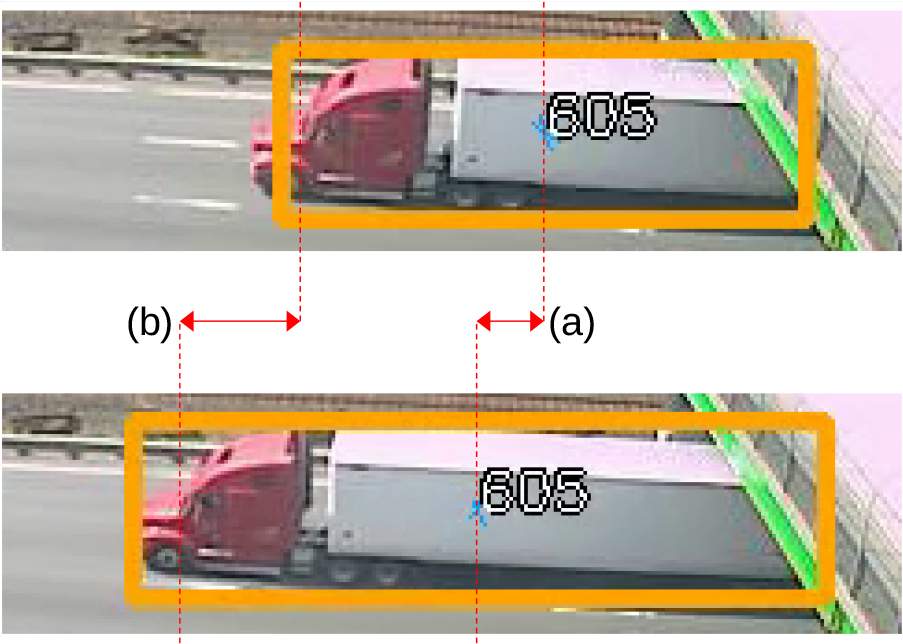

A second issue is that $A^{\prime}_{i}(t)$ is not dimensionless. Its dimension depends on the frame rate, traffic speed patterns, the distance to the camera, and other factors. This is managed by considering $A_{i}^{\prime}(t)$ as potentially anomalous whenever its value is equal to or higher than the $P_{k}$ -th percentile of the anomaly values observed during the last $F$ frames.

Also, there is an issue when vehicles take several frames to gradually go from being partially occluded to fully visible: the larger the vehicle, the lower the apparent velocity. This happens because the object detector defines the vehicle’s boundary relative to its visible portion, and the center of the bounding box is taken as a proxy for the position. As larger and larger portions of the vehicle become visible in the image, the bounding box will gradually grow, and the velocity of the center of the vehicle will be slower than if the vehicle were fully visible (see Fig. 2). This issue can happen with any road occlusion such as bridges or large trees, but the effect is especially acute at the borders of the camera’s field of view, since in general there will be one or more borders where traffic will appear or disappear.

This might not be a problem unto itself, because it just means that velocities will be generally slower near borders and road occlusions. However, the severity of the effect varies greatly according to apparent vehicle size, so large trucks will have significantly slower velocities than cars and motorcycles, and for longer stretches of road. When comparing these velocities of large trucks to cars, there will be a greater probability of marking the former as anomalous. To mitigate this effect, border correction is performed, i.e. filtering out as not potentially anomalous any $A_{i}(t)$ whose underlying bounding box is close to the border. As a quantitative heuristic, we apply this criterion with a bounding box if any of its edges is closer to the border than 5% of its smallest edge.

Table 1

Parameters of the model

Parameter description	Value(s)
Number of nearest neighbors	$N=5$
Anomaly threshold: percentile	$P_{k}\in\{0.85,0.9,0.95,0.98,0.99\}$
Anomaly threshold: severity	$S\in\{3,4,5,6\}$
Anomaly threshold: number of frames	$F=60$
Apply border correction	No/yes
Apply bounding box similarity	No/all vehicles/small vehicles
Bounding box similarity: network	Resnet18, resnet101, vgg11, vgg19
Bounding box similarity: threshold	$T\in\{0.1,0.2,0.3,0.4,0.5\}$

The final step is to classify a potentially anomalous $A^{\prime}_{i}(t)$ as actually anomalous if any of the following two conditions are met:

•

Its value relative to the $P_{k}$ -th percentile is larger than a specific ratio $s$ : $A_{i}^{\prime}(t)\geqslant s\cdot P_{k}$ .

•

A long record of potentially anomalous values has been accumulated for the vehicle during a number of consecutive frames. This criterion depends on the characteristic time and size scales of the vehicles in the traffic scene.

Figure 2 shows a vehicle position estimation example: the vehicle position is estimated as the center of the bounding box. Velocity is estimated as difference between such positions (a). For comparison, in this figure the real velocity (b) is estimated by measuring the distance between frames for a specific keypoint (the windshield). As a result, large vehicles appearing into the scene may be erroneously considered to be slower than they really are, thus potentially flagging them as anomalous. This problem is most common along the borders of the image, and a pragmatic and effective solution is to ignore vehicles near the border.

4. Experiments and results

The proposed model has been evaluated with a dataset several times, testing various configurations. The source code is available at http://github.com/jdfr/anomalous_trajectory_detection_2023.

4.1 Methods

All proposals have been implemented using Python (https://www.python.org/) language, tracking stage linear sum assignment is solved by using SciPy’s (https:// scipy.org/) implementation and video snippets are processed by using OpenCV library (https://opencv.org/).

Yolov5, a well-known neural network model, is used as the object detection method. We only need to detect vehicles, so yolov5’s configuration has been altered to only return objects from the following classes: car, motorcycle, bus, and truck. Most Yolov5 configuration values are the standard (particularly $r_{\min}=0.25$ ) but since the object detection model sometimes wrongly detects cars instead of truck cabins, even inside a bounding box of the whole truck, object class is disregarded in the non-maximum-suppression algorithm.

Concerning anomaly detection parameters, the number of nearest neighbors to check if a trajectory is anomalous (size of $D_{i}^{N}(t)$ ) should be small. Otherwise, $D_{i}^{N}(t)$ is likely to contain many vehicles with very different trajectories for a long time after initialization. A number of preliminary, non-exhaustive experiments were performed with different values for the number of nearest neighbors ( $N$ ), finding the method prone to false positives in the first processed frames when using high values for $N$ . Setting $N=5$ provided for a reasonable performance compared to other values. Regarding the number of frames the algorithm keeps track of past detections ( $F$ ), experiments show better results when no data are forgotten for the duration of each video sequence. To classify a trajectory as potentially anomalous, $P_{k}$ parameter is used, so a value equal to or above it will flag the trajectory as anomalous.

Table 1 provides a concise view of the parameters of the model. Exhaustive search to determine parameters $N$ and $F$ was deemed impractical, so preliminary experiments were conducted to settle on values providing reasonable performance. For the other parameters, this table provides the ranges of tested values. See the following subsections for an in-depth exploration of the parameters in the Table. Regarding the conditions to consider vehicles as actually anomalous:

•
For vehicles having very large $A_{i}^{\prime}(t)$ values, an array of experiments has been conducted to tune the values of parameters $s$ and $P_{k}$ (see Section 4.3).
•
For vehicles keeping anomalous $A_{i}^{\prime}(t)$ values for extended periods of time, they are marked as actually anomalous if they keep anomalous $A_{i}^{\prime}(t)$ for 60 or more consecutive frames (corresponding to 2–3 seconds for the videos used in the experiments). In preliminary experiments, shorter extents of time translated into increased false positive rates, while longer extents of time led to reduced detection rates of true positive frames.

4.2 Datasets

Different videos selected from several datasets have been considered in the experiments. With these sequences, the performance of the model can be analyzed under different anomaly conditions related to wrong-way driving, such as a vehicle in the opposite direction or backing onto roads. Videos from four datasets were used:

•
First subset: three videos from a project [69] dealing with anomalous trajectory detection in traffic videos. The selected sequences are a real video (Clip from 02:10 to 02:31 in this Youtube video: https://youtu.be/BF3WuB-7iPo) noted as Video1 that shows a vehicle backing onto a busy road, and two videos synthesized with CARLA [70] (noted as Video2, and emphVideo4), both of them depicting a car doing counterflow driving. All three videos depict anomalous vehicles.
•
Second subset: Six videos from the Ko-PER Intersection dataset [71]: the sequences 1a-SK_1, 1a-SK_4, 2-SK_1, 2-SK_4, 3-SK_1, and 3-SK_4. Each pair of sequences with the same prefix and ending in _1 or _4 are recordings of the same scene from two different cameras, providing valuable validation of the model for scenes that should result in similar predictions in each case. Videos with prefixes 1a- and 3- do not actually show anomalous trajectories, while videos with prefix 2- show a vehicle that waits in the middle of the intersection to turn. To test the proposed methodology, that vehicle has been considered anomalous.
•
Third subset: Three videos from the 2014 CDNET dataset [72]: the sequences highway, streetLight, and traffic. All of them were taken from a camera looking at traffic on a straight road from different orientations (respectively: from the front, side, and rear). None of them show anomalous vehicles.
•
Fourth subset: Fifteen videos from the training set of the 2021 NVidia AI City Challenge [73], Track #4: videos 1, 2, 3, 5, 9, 13, 14, 17, 20, 22, 25, 33, 39, 41, and 50. These were selected with two criteria in mind: avoiding views of intersections and avoiding videos where the off-the-shelf object detector struggles to detect vehicles reliably (see Section 4.3.6 for details on these limitations). Each video is 15 minutes long. For practical reasons, each video was divided into 15 segments, approximately one minute each, resulting in 225 video clips. At 30 frames per second, these one-minute clips average 1800 frames each. It is worth noting that this dataset is designed as a challenge to detect traffic accidents where anomalous vehicles pull up to the roadside. However, our proposed method does not detect this type of anomaly, but wrong-way anomalies. Because of this, none of these one-minute video clips has any anomalous frame for our purposes.

Thus, we have four subsets of video sequences, 237 videos in total. The fourth one (the video clips from the NVidia AI City Challenge dataset) represents the vast majority of the videos (225), but they have no anomalous frames. The first three subsets represent a mix of videos of various lengths, some depicting vehicles in wrong-way trajectories. To effectively use computing resources, we will use videos from these first three subsets to evaluate the system’s performance under a wide variety of configurations. Once the best configuration is selected, we will also evaluate its performance with the fourth subset (the video clips from the AI City Challenge).

It should be noted that datasets containing many examples of videos with wrong-way, anomalous trajectories can be found for videos taken from dashcams. However, we do not know of such a dataset with videos taken from traffic cameras, and videos taken from dashcams are not suitable for the proposed model. While the model is designed for views of non-intersecting roads, videos from intersections depicting vehicles that might be considered anomalous have been included in the experiments, as described above. For comparison, videos of intersections without anomalous trajectories have also been included (it should be noted, however, that the proposed model does not work well for these).

Table 2
Mean values for precision, recall, and Jaccard index, across videos from the first three subsets, for each combination of $s$ and $P_{k}$

$P_{99}$ $P_{98}$ $P_{95}$ $P_{90}$ $P_{85}$

P R J P R J P R J P R J P R J

$s=3$ – – – – – – 0.409 0.263 0.219 0.275 0.327 0.171 0.222 0.335 0.147

$s=4$ – – – – – – 0.445 0.259 0.220 0.290 0.298 0.163 0.244 0.330 0.146

$s=5$ – – – – – – – – – 0.319 0.289 0.158 0.249 0.295 0.139

$s=6$ – – – – – – – – – – – – 0.265 0.257 0.133

For each video, ground truth is determined by manually labeling each frame of each video as being anomalous/not anomalous (in all instances, videos with anomalies had at most one anomalous car in each frame). At evaluation time, for each frame in a video:

•
If the frame was labeled as non-anomalous, it is a true negative (TN) if no trajectory was considered as actually anomalous by the model at that frame; false positive (FP) otherwise.
•
If the frame was labeled as anomalous, it is a true positive (TP) if exactly one trajectory was considered as anomalous by the model at that frame; false negative (FN) otherwise.

With these considerations, standard measures such as precision $P$ , recall $R$ , and Jaccard index $J$ (which can be interpreted as a combination of the first two) can be computed for each video:

$\displaystyle P=\frac{TP}{TP+FP}$ $\displaystyle R=\frac{TP}{TP+FN}$ (12) $\displaystyle J=\frac{TP}{TP+FP+FN}$

Please note that these formulae might become indeterminate for videos with no frames labeled as anomalous. In such cases, if there are no false positives, the algorithm performs perfectly. Because of this, when these formulae are indeterminate, the value is set to 1 if $FP=0$ (0 if $FP>1$ ). Since we are interested in being able to flag whole videos as either having or not having anomalous trajectories, TP and FP frames are considered to be more significant than FN frames. Therefore, for our purposes, precision and the Jaccard index are deemed to be more significant than recall. Also, as long as the TP frame count is not zero for videos whose ground truth includes anomalous frames, the model is considered to have correctly predicted the video as containing anomalous vehicles.

Labeling anomalies at the bounding box level might be a more precise way to measure performance, but the proposed methodology works reasonably well for the use case exposed here.
4.3 Results

	$P_{99}$	$P_{98}$	$P_{95}$	$P_{90}$	$P_{85}$
	P	R	J	P	R	J	P	R	J	P	R	J	P	R	J
$s=3$	–	–	–	–	–	–	0.409	0.263	0.219	0.275	0.327	0.171	0.222	0.335	0.147
$s=4$	–	–	–	–	–	–	0.445	0.259	0.220	0.290	0.298	0.163	0.244	0.330	0.146
$s=5$	–	–	–	–	–	–	–	–	–	0.319	0.289	0.158	0.249	0.295	0.139
$s=6$	–	–	–	–	–	–	–	–	–	–	–	–	0.265	0.257	0.133

Experiments were carried out to evaluate the performance of the model under various combinations of parameters. Because of the large number of parameters and unknowns, it was impractical to perform an exhaustive evaluation of performance for all possible combinations of parameters, with a large number of video sequences. Instead, a staggered approach was followed, conducting three studies of the performance of the system:

•
First, reasonable values were sought for the parameters $s$ and $P_{k}$ of the anomaly detection model by disabling advanced techniques (border correction and bounding box similarity), testing all possible combinations of parameters $s\in\{3,4,5,6\}$ and $P_{k}\in\{0.85,0.9,0.95,0.98,0.99\}$ .
•
With established values for $s$ and $P_{k}$ , the model was tested with all combinations of using/not using border correction, not using bounding box similarity, or using bounding box similarity with various deep classifiers (resnet18, resnet101, vgg11 and vgg19) at a range of similarity thresholds: $\{0.1,0.2,0.3,0.4,0.5\}$ . This range was selected by manually examining the similarity values at the beginning of a few videos.
•
A comparison of the performance yielded by other state-of-the-art LSAP-based trackers. In particular, our proposal is compared to two well-known methods: SORT and BYTE. Also, we study its performance in videos with added rain and snow.

The first two studies (Sections 4.3.1 and 4.3.2) require an extensive array of experiments. Because of this, the system’s performance with different configurations in these two studies is conducted with the videos from the first three subsets. Once the best configuration is determined, the third study (Sections 4.3.4 and 4.3.5) evaluates its performance on all videos from the four subsets. For more details on the four subsets of videos, see Section 4.2.
4.3.1 Finding optimal values for $s$ and $P_{k}$

Results for the first stage are shown in Table 2. It shows mean values for precision, recall, and Jaccard index, across videos from the first three subsets, for each combination of $s$ and $P_{k}$ . Cells with “ $-$ ” correspond to configurations resulting in one or more videos with actual anomalies but no TP frames. The best values for each performance measure are in bold, computing the average values across all videos from the first three subsets (see Section 4.2) for precision, recall, and Jaccard index. Since one of the applications of the model might be to flag video snippets as containing anomalous vehicle behaviors, it is deemed especially important to tune the model so that no video actually depicting anomalous vehicles has zero TP frames, since that would mean that video to be predicted as having non-anomalous trajectories at all. Consequently, parameter combinations leading to this are not considered adequate (even if they have better performance values than others). From Table 2, it can be seen that the best configuration in terms of precision and Jaccard index corresponds to $s=4$ and $P_{k}=0.95$ .

Table 3
Mean precision, recall, and Jaccard index, across videos from the first three subsets, for configurations with $s=4$ , $P_{95}$ with border correction

	resnet18			resnet101			vgg11			vgg19
	P	R	J	P	R	J	P	R	J	P	R	J
$T=0.1$	–	–	–	–	–	–	–	–	–	–	–	–
$T=0.2$	0.512	0.240	0.238	–	–	–	–	–	–	–	–	–
$T=0.3$	0.503	0.290	0.281	0.521	0.288	0.285	–	–	–	–	–	–
$T=0.4$	0.494	0.298	0.285	0.494	0.298	0.285	0.499	0.282	0.280	0.426	0.199	0.196
$T=0.5$	0.507	0.298	0.284	0.507	0.298	0.284	0.413	0.213	0.201	0.405	0.213	0.201

Table 4

Same as Table 3, but applying bounding box similarity only to vehicles of small apparent size

	resnet18			resnet101			vgg11			vgg19
	P	R	J	P	R	J	P	R	J	P	R	J
$T=0.1$	0.519	0.287	0.282	0.520	0.287	0.282	0.530	0.277	0.274	0.519	0.277	0.274
$T=0.2$	0.516	0.290	0.284	0.525	0.290	0.284	0.534	0.277	0.274	0.519	0.287	0.282
$T=0.3$	0.507	0.298	0.284	0.533	0.290	0.285	0.517	0.290	0.284	0.517	0.290	0.284
$T=0.4$	0.508	0.298	0.284	0.507	0.298	0.284	0.550	0.313	0.306	0.543	0.316	0.305
$T=0.5$	0.507	0.298	0.284	0.508	0.298	0.284	0.508	0.298	0.284	0.507	0.298	0.284

Table 5

Same as Table 3, but for configurations without border correction

	resnet18			resnet101			vgg11			vgg19
	P	R	J	P	R	J	P	R	J	P	R	J
$T=0.1$	–	–	–	–	–	–	–	–	–	–	–	–
$T=0.2$	0.526	0.251	0.241	0.550	0.283	0.279	–	–	–	–	–	–
$T=0.3$	0.424	0.223	0.203	0.514	0.324	0.304	0.477	0.248	0.237	0.540	0.245	0.236
$T=0.4$	0.448	0.259	0.222	0.448	0.259	0.222	0.481	0.292	0.280	0.491	0.292	0.282
$T=0.5$	0.446	0.259	0.221	0.445	0.259	0.220	0.507	0.315	0.294	0.507	0.314	0.293

Table 6

Best performance of the proposed method with different combinations of border correction and bounding box similarity

Border correction	Bounding box similarity	P	R	J
No	No	0.445	0.259	0.220
Yes	No	0.507	0.298	0.284
No	All vehicles	0.550	0.283	0.279
No	Small vehicles	0.463	0.229	0.216
Yes	All vehicles	0.512	0.240	0.238
Yes	Small vehicles	0.550	0.313	0.316

4.3.2 Effects of border correction and bounding box similarity

For the second stage, with the first parameters fixed to $s=4$ and $P_{95}$ , the performance of the system was studied when using both border correction and bounding box similarity with various configuration of deep network and threshold $T$ , using the videos from the first three subsets (see Section 4.2). Results can be seen in Table 3, applying bounding box similarity for all vehicles, for each combination of backbone and similarity threshold $T$ . Cells without values correspond to configurations resulting in one or more videos with actual anomalies but no TP frames. The best values for each performance measure are in bold. values for $T=0.4$ are slightly better than for $T=0.5$ for resnet18 and resnet101. Additionally, for $T=0.4$ , resnet18 and resnet101 are tied for recall and the Jaccard index. ResNet models were found to produce better results than VGG models, with deeper models providing little to no benefit over shallower, more efficient models. Table 4 shows that with small vehicles it is slightly preferable to use VGG models, although the value $T=0.4$ is still preferable. This trend changes if we look at configurations without border correction in Table 5. In these we observe that the values $T=0.2$ for precision and $T=0.3$ for recall and Jaccard index are significantly better. On the whole, very few configurations with border correction and bounding box similarity had either better precision or better recall than using border correction alone, but one of them was found to have a better average value for the Jaccard index, which can be considered as a combination of the other two.

Table 7
Detailed performance values (TP, FP, TN, FN, precision, recall, Jaccard index) for the best configuration

	vid.1	vid.2	vid.4	1a-SK_1	1a-SK_4	2-SK_1	2-SK_4	3-SK_1	3-SK_4	highway	streetLight	traffic
TP	60	7	3	0	0	395	108	0	0	0	0	0
FP	19	1	0	136	36	14	0	21	39	0	3	0
TN	168	1046	807	2283	2383	512	521	999	981	1700	3197	1570
FN	66	91	139	0	0	26	318	0	0	0	0	0
P	0.759	0.875	1	0	0	0.966	1	0	0	1	0	1
R	0.476	0.071	0.021	0	0	0.938	0.254	0	0	1	0	1
J	0.414	0.071	0.021	0	0	0.908	0.254	0	0	1	0	1

The purpose of applying bounding box similarity is to limit errors in trajectory tracking. Given that the model already performed well for vehicles with large apparent sizes, we hypothesized that the relatively small performance improvement of bounding box similarity was the result of excessive disruption to the tracking of vehicles with large apparent sizes. In order to test this hypothesis, all experiments with bounding box similarity were run again, but restricting its application to vehicles of small apparent size (as described in Section 3.2, vehicles whose smaller side is below 2.5% of the largest side of the image). Results for this array of experiments are shown in Table 4. In this case, results improve significantly over using border correction alone for most configurations. However, no backbone and no threshold $T$ seem to consistently outperform others, although all configurations with the best performance used VGG backbones.

The performance of the model was also investigated for configurations with bounding box similarity but not border correction. When applying bounding box similarity only for small vehicles with apparent size, results were consistently worse than also using border correction (data not shown). However, when applying it to vehicles of any size, some configurations outperformed border correction alone, as shown in Table 5, possibly because boxes of vehicles that are appearing/disappearing naturally tend to have lower similarity scores, thus having an effect similar to border correction. In this case, ResNet models outperformed VGG models, and deeper models produced better results.

According to these results, we determine the best configuration: use border correction and bounding box similarity just for vehicles of small apparent size, with threshold $T=0.4$ and network vgg11. These results are shown in Table 6, where the results of the other tables discussed in this section are included in an ablation study (third, fifth and sixth rows are best results from Tables 5, 3 and 4, respectively), showing the relative performance gains of using each configuration of parameters. For the sake of completeness, additional experiments were carried out to test the system’s performance with all possible combinations of using/not using border correction and bounding box similarity. While the table shows progression in performance from the vanilla system to the best combination of border correction and bounding box similarity, this progression does not seem to represent a linear progression of gains in performance, reflecting that the effects of both border correction and bounding box similarity interact in non-trivial ways.

Figure 3.

Graphic depiction of the results for our best method with border correction and bounding box similarity (see Section 4.3.3 for details).

Figure 4.

Predictions made for different videos in an specific instant. Left to right: Video1 (frame 247), Video4 (frame 873) and seq. 2 SK_4 (frame 672).

4.3.3 Best configuration

The configuration with the best precision and Jaccard index is the one with border correction and bounding box similarity applied only to vehicles with small apparent size, using the vgg11 backbone, and similarity threshold $T=0.4$ . For this configuration, Table 7 shows per-video performance figures, for all videos from the first three subsets (see Section 4.2) using border correction and bounding box similarity applied only for vehicles with small apparent size, backbone vgg11, and similarity threshold $T=0.4$ . Please note that formulae for P, R, and J might be indeterminate for videos with no frames labeled as anomalous. In such cases, we set the value to 1 if $FP=0$ , and 0 otherwise: the algorithm performed perfectly in such videos if there were no false positives. As explained in Section 4.2, the model struggles with videos of intersections, but videos for intersections (1a-SK_1, 1a-SK_4, 2-SK_1, 2-SK_4, 3-SK_1, and 3-SK_4) are included for comparison.

The information in the table about the TP, FP, TN and FN frames is also shown in Fig. 3 in a more visual way: each video is represented by a horizontal bar whose length is its number of frames. These are the videos used to compute the statistics for Tables 2–6. For each video, its length is expressed in frames. Frames can be labeled as TP (bright red), FP (dark red), TN (bright green) and FN (dark green). Actually anomalous frames (ground truth) are the union of TP and FN frames, comprising one or two contiguous segments in several videos. For Video1, the anomalous segments are the periods when a car is backing onto a busy road. For Video2 and Video4, the anomalous segment includes cars engaging in counterflow driving. For seq. 2-SK_1 and SK_4, the anomalous segment depicts a car stopped in the middle of an intersection, flanked by fast traffic. All other videos lack anomalous segments. The bar is colored according to the status of each frame: TP frames are bright red, FP frames are dark red, TN frames are bright green, and FN frames are dark green. Given the above configuration, the frame-by-frame results for the tested video sequences are shown in Fig. 3. Video1, Video2, seq. 2, cam. SK_1 and seq. 2, cam. SK_4 contain real, well-detected anomalies (i.e. true positives). False positives typically represent very brief segments, and by analyzing the frames in which the false positives appear, two cases are deduced: the first time that, after the start of the sequence, any vehicle uses a lane of the road or an intersection, the system is likely to mark those vehicles as anomalous; the second case is when many overlapping trajectories accumulate in the same area (e.g. an intersection) due to the comparison between the trajectories of some vehicles with very different overlapping trajectories.

Table 8
Mean values for precision, recall, and Jaccard index across all videos, for configurations with $s=4$ , $P_{95}$ and using either SORT or BYTE instead of the custom tracking algorithm

	SORT			BYTE			OURS
	P	R	J	P	R	J	P	R	J
No border correction	0.541	0.532	0.530	0.460	0.453	0.452	0.592	0.583	0.581
Border correction	0.577	0.568	0.567	0.526	0.512	0.512	0.619	0.607	0.606

Table 9

Pairwise Cochran’s Q tests between distributions of correctly classified frames for the best method with border correction and all other methods in Table 8

		OURS, border correction		Cochran’s Q statistic	$p$ -value
		Correct	Incorrect
SORT, border correction	Correct	415912	80	215.112	1.05E-48
	Incorrect	402	1764
BYTE, border correction	Correct	413956	197	1827.757	0
	Incorrect	2358	1647
SORT, no border correction	Correct	415235	342	382.244	4.03E-85
	Incorrect	1079	1502
BYTE, no border correction	Correct	413601	380	1759.744	0
	Incorrect	2713	1464
OURS, no border correction	Correct	415602	320	148.899	3.01E-34
	Incorrect	712	1524

Specific vehicles with trajectories classified as anomalous by the model are shown in Fig. 4:

•

Left image: a vehicle is backing onto a busy road.

•

Center image: a vehicle driving in opposite direction.

•

Right image: a vehicle is stopped in the middle of a busy intersection.

Cyan-colored lines on the center of each vehicle bounding box represent the $N=5$ nearest neighbors involved in obtaining $A_{i}(t)$ value for each vehicle at time $t$ . Each line goes from the center of the vehicle’s bounding box to the center of the bounding box of one of the nearest neighbors (these bounding boxes are typically from past frames, and they are not shown in the current frame to avoid cluttering the scene).

4.3.4 Comparison with other models

Finally, the model was tested by substituting the custom tracker with two well-known generic LSAP-based trackers: SORT and BYTE. In this case, once the best configuration has already been established for our proposal, we test the performance of the models with all videos, including the fourth subset (see Section 4.2) with 225 one-minute video clips. As border correction is applied outside the tracking algorithm, both trackers were tested with and without border correction, finding that border correction can enhance the performance of both. Without border correction, SORT is superior to BYTE in all metrics. However, BYTE’s metrics are more significantly boosted than SORT’s, to the point that BYTE’s precision surpasses SORT’s with border correction, while its recall and Jaccard index get close but do not surpass SORT’s.

Table 8 shows average precision, recall and Jaccard index across all videos for six different possibilities: our best configuration (with vgg11 and similarity threshold $T=0.4$ , only for vehicles with small apparent size), SORT and BYTE, each one either with or without border correction, from all six evaluated methods. The best configuration of the custom tracking algorithm outperforms both SORT and BYTE for all three metrics in both modalities (with and without border correction). As border correction is applied outside of the tracking algorithm, tests with and without border correction were carried out. For comparison, values are shown for the best configuration with our custom tracker (using box similarity with vgg11 and similarity threshold $T=0.4$ , only for vehicles of small apparent size). The best values for each performance measure are in bold.

Figure 5.

Lower-left corner of the frame 150 of Video1 with detections and trajectory identifier, same excerpt with synthetically added rain, and with snow.

To validate the statistical significance of these results, we perform an array of statistical tests to validate that the distributions are different. However, in order to have a higher level of statistical significance, the statistical tests are performed not at the level of whole videos (237 videos in total) but over the population of all frames from all videos (418158 frames in total). At the frame level, a useful way to characterize each of these six methods is to consider the associated Boolean distribution that represents the set of frames correctly classified by that method (i.e., frames being either TP or TN). The Cochran’s Q test [74] assesses whether there is a statistically significant difference between binary distributions. To test whether these distributions are statistically different, we run pairwise Cochran’s Q tests between the distribution for the best method and all other methods. The resulting very low $p$ -values (presented in Table 9, together with the contingency table for each test) mean that the distribution of correctly classified frames with the best method is statistically different from the other ones with a high level of confidence. For each test, the contingency table (number of frames correctly/incorrectly in each test) is provided in the third and fourth columns, and the resulting Cochran’s Q statistic and associated $p$ -value in the fifth and sixth columns. In all cases, the $p$ -value is effectively 0, meaning that the distributions are statistically significant.

4.3.5 Rain and snow

As an anomaly detection system for outdoor cameras, it is also desirable to test its performance for traffic videos with rain and snow. The Aalborg dataset [75] provides real traffic videos in raining and snowing conditions. However, only select frames (i.e. not the full videos) are readily available, and all videos from this dataset depict intersections rather than highways. Instead, we tested the system’s performance by artificially adding rain and snow to all the videos (from all four subsets) using a publicly available library (https:// github.com/aleju/imgaug). Figure 5 shows the lower-left corner of frame 150 for Video1 with synthetically added rain and snow. Performance results (average precision, recall and Jaccard index across all videos from all four subsets) are shown in Table 10: rain and snow degrade performance, but not dramatically so.

Table 10
Comparison of mean values for precision, recall, and Jaccard index, across all videos, for the best method in different conditions

Weather	P	R	J
No changes	0.619	0.607	0.606
Added rain	0.582	0.572	0.572
Added snow	0.559	0.546	0.546

4.3.6 Limitations

The previous sections explore the model’s performance of the model under good favourable conditions. However, it is also necessary to discuss the limitations of the proposed model. An important restriction is that all used videos have reasonably high framerates, translating into relatively small and smooth vehicle displacements from one frame to the next. When applying the method to videos with significantly lower framerates (from half to a third), we found the performance to be substantially poorer, as the various tested tracking subsystems failed to accurately track trajectories for very fast vehicles and vehicles of small apparent size. As a result, the statistical distribution of anomaly values significantly changed, dramatically increasing the number of false negatives.

Other limitations come from using a generic object detector (yolov5) as the detection stage: as the detector was trained on generic image datasets with very limited ranges of traffic conditions, the detecting performance is severely degraded in various scenarios:

•
For vehicles of very small apparent size (e.g. when using a wide camera aperture, or when cameras are placed relatively high).
•
For overlapping vehicles of small apparent size (e.g. with very dense traffic, when the viewing angle does not minimize vehicle overlapping in the image).
•
For unfocused vehicles (this is especially serious for vehicles of small apparent size).
•
For scenes with bad illumination (e.g., videos recorded at night).

Finally, the development of the system has been done with flexibility and ease of data collection in mind, resulting in a Python implementation that is significantly slower than it could be. The full-fledged system (using bounding box similarity and border correction) takes about 3.5 minutes to process a one-minute video clip in a machine with an Intel i7 processor and a 3080 GPU. Consequently, it cannot be used for real-time detection in its current state.
5. Conclusions

An approach to detect anomalous, wrong-way vehicle trajectories from traffic video sequences has been proposed in this work. This proposal computes the video frame by frame, and it is based on the velocity vectors of those detected trajectories. The proposed methodology is composed of several steps. First, the detection of the vehicles that appear in a frame is addressed by a component base on a deep learning model. Then, the trajectories of the detected vehicles are tracked. To enhance the performance of the tracker, the impact of adding techniques such as border correction and bounding box similarity has been analyzed. Once trajectories have been tracked, the velocity vector of each trajectory is computed and compared with velocity vectors from other spatially adjacent trajectories. This comparison aims to detect those unusual (that is, anomalous) trajectories.

Different experiments have been conducted to test the performance of the approach. A set of synthetic and real sequences and several methods from state-of-the-art have been considered in the comparison. Results demonstrate our proposal is suitable for detecting anomalous trajectories such as vehicles driving in opposite directions or backing onto a road.

Future works include the addition of a specific procedure to manage intersecting roads. In these situations, the velocity vectors of the normal trajectories exhibit two or more different modes associated with the allowed directions for the cars to traverse the crossroads. In other words, the velocity vector distribution is multimodal. This adaptation could be done by modeling each of the modes with a probabilistic mixture component, or any other unsupervised learning model that finds the clusters in a multimodal input distribution.

Another line of future work is the optimization of the implementation: if it were fast enough to be applied in real-time, it would allow for the online detection of anomalies, as at each time step, no information is used to determine if a trajectory is anomalous. This can be accomplished by reimplementing the deep learning parts of the pipeline in TensorRT, as well as carefully reimplementing the data structures used for trajectory tracking and anomaly detection, bounding their sizes and optimizing them for fast access times.

While the system as currently proposed works reasonably well in various weather conditions, another avenue for improvement is to optimize the off-the-shelf object detector. It can be fine-tuned to reliably detect individual vehicles in currently problematic scenarios such as nighttime, unfocused cameras, small apparent size and the high overlapping of vehicle silhouettes that can arise from a combination of the camera angle and dense traffic. In a related line of work, it should also be possible to tweak the trajectory subsystem to track trajectories at lower framerates reliably. This would enable application in real-time with less optimization work, and also application to video feeds that are naturally available at lower framerates.

To test other classification approaches we plan to test dynamic neural classifications [76], fast learning [77] and ensembles of classifiers [78], as well as to study the possibility of processing 3D data [79, 80].

Footnotes

Acknowledgments

This work is partially supported by the University of MÃ¡laga under grant B1-2022_14. This work is partially supported by the Ministry of Science, Innovation and Universities of Spain under grant RTI2018-094645-B-I00, project name Automated detection with low-cost hardware of unusual activities in video sequences. It is also partially supported by the Autonomous Government of Andalusia (Spain) under project UMA18-FEDERJA-084, project name Detection of anomalous behavior agents by deep learning in low-cost video surveillance intelligent systems. It is also partially supported by the Autonomous Government of Andalusia (Spain) under project UMA20-FEDERJA-108, project name Detection, characterization and prognosis value of the non-obstructive coronary disease with deep learning. All of them include funds from the European Regional Development Fund (ERDF). It is also partially supported by the University of Malaga (Spain) under grants B1-2019_01, project name Anomaly detection on roads by moving cameras; B1-2019_02, project name Self-Organizing Neural Systems for Non-Stationary Environments; and B1-2021_20, project name Detection of coronary stenosis using deep learning applied to coronary angiography. The authors thankfully acknowledge the computer resources, technical expertise and assistance provided by the SCBI (Supercomputing and Bioinformatics) center of the University of Málaga. They also gratefully acknowledge the support of NVIDIA Corporation with the donation of two Titan X GPUs. The authors also thankfully acknowledge the grant of the Universidad de Málaga and the Instituto de Investigación Biomédica de Málaga y Plataforma en Nanomedicina-IBIMA Plataforma BIONAND.

References

Avola

Cascio

Cinque

Foresti

Pannone

. Machine learning for video event recognition. Integrated Computer-Aided Engineering. 2021; 28(3): 309-332.

Carranza-García

Galán-Sales

Luna-Romera

Riquelme

. Object detection using depth completion and camera-LiDAR fusion for autonomous driving. Integrated Computer-Aided Engineering. 2022 5; 29: 1-18.

Liu

Liao

Ren

. High-Level Semantic Feature Detection: A New Perspective for Pedestrian Detection. 2019 IEEE/CVF Conference on Computer Vision and Pattern Recognition (CVPR). 2019. pp. 5182-5191.

Tomè

Monti

Baroffio

Bondi

Tagliasacchi

Tubaro

. Deep convolutional neural networks for pedestrian detection. Signal Processing: Image Communication. 2016; 47: 482-489.

Herdade

Kappeler

Boakye

Soares

. Image captioning: Transforming objects into words. Advances in Neural Information Processing Systems. 2019; 32.

Sehgal

Mandan

. Automated image capturing using CNN and RNN. International Journal of Research in Engineering, Science and Management. 2022; 5(1): 13-17.

Lee

. CNN-based single object detection and tracking in videos and its application to drone detection. Multimedia Tools and Applications. 2021; 80(26): 34237-34248.

Kashika

Venkatapur

. Automatic tracking of objects using improvised Yolov3 algorithm and alarm human activities in case of anomalies. International Journal of Information Technology. 2022; 1-7.

Liu

Weng

Yang

. Rotated region based CNN for ship detection. In: 2017 IEEE International Conference on Image Processing (ICIP). IEEE; 2017. pp. 900-904.

10.

Daranda

Dzemyda

. Reinforcement learning strategies for vessel navigation. Integrated Computer-Aided Engineering. 2022; (Preprint): 1-14.

11.

Benamara

Val-Calvo

Alvarez-Sanchez

Diaz-Morcillo

Ferrandez-Vicente

Fernandez-Jover

, et al. Real-time facial expression recognition using smoothed deep neural network ensemble. Integrated Computer-Aided Engineering. 2021; 28(1): 97-111.

12.

Wang

Bai

. Regional parallel structure based CNN for thermal infrared face identification. Integr Comput-Aided Eng. 2018 jan; 25(3): 247-260. Available from: doi: 10.3233/ICA-180560.

13.

Fernández

García-González

Benítez-Rochel

Molina-Cabello

López-Rubio

. Anomalous Trajectory Detection for Automated Traffic Video Surveillance. In: International Work-Conference on the Interplay Between Natural and Artificial Computation. Springer; 2022. pp. 173-182.

14.

Sousa

Teixeira

Carneiro

Nunes

Novais

. Knowledge-based decision intelligence in street lighting management. Integrated Computer-Aided Engineering. 2022; (Preprint): 1-19.

15.

Patil

Prabhushetty

. A Survey on Human Action Recognition and Detection Techniques. In: ICT Analysis and Applications. Springer; 2022. pp. 157-165.

16.

Kong

. Human action recognition and prediction: A survey. International Journal of Computer Vision. 2022; 130(5): 1366-1401.

17.

Foresti

Scagnetto

. An integrated low-cost system for object detection in underwater environments. Integrated Computer-Aided Engineering. 2022; (Preprint): 1-17.

18.

Gasienico-Jozkowy

Knapik

Cyganek

. An ensemble deep learning method with optimized weights for drone-based water rescue and surveillance. Integrated Computer-Aided Engineering. 2021; 28(3): 221-235.

19.

Manickam

Samuel

. Automatic detection technology for sports players based on image recognition technology: The significance of big data technology in China’s sports field. Annals of Operations Research. 2022; 1-18.

20.

Sharma

Shah

Prakash

. A Pilot Study on Human Pose Estimation for Sports Analysis. In: Pattern Recognition and Data Analysis with Applications. Springer; 2022. pp. 533-544.

21.

Ying

Zhou

Degani

Sacks

. A two-stage recursive ray tracing algorithm to automatically identify external building objects in building information models. Computer-Aided Civil and Infrastructure Engineering. 2022 7; 37: 991-1009.

22.

Pan

Yang

. Image-based monitoring of bolt loosening through deep-learning-based integrated detection and tracking. Computer-Aided Civil and Infrastructure Engineering. 2022 8; 37: 1207-1222.

23.

Zhang

Wang

KCP

Liu

Zhan

Yang

Wang

, et al. Intelligent pixel-level detection of multiple distresses and surface design features on asphalt pavements. Computer-Aided Civil and Infrastructure Engineering. 2022 11; 37: 1654-1673.

24.

. Recognizing object surface materials to adapt robotic disinfection in infrastructure facilities. Computer-Aided Civil and Infrastructure Engineering. 2022 10; 37: 1521-1546.

25.

Shen

Yan

Xiong

. Deep learning-based object identification with instance segmentation and <b> pseudo-LiDAR point cloud for work zone safety </b>. Computer-Aided Civil and Infrastructure Engineering. 2021 12; 36: 1549-1567.

26.

Luo

Yan

Ren

Bai

, et al. Autonomous detection of damage to multiple steel surfaces from 360∘ panoramas using deep neural networks. Computer-Aided Civil and Infrastructure Engineering. 2021 12; 36: 1585-1599.

27.

Rafiei

Khushefati

Demirboga

Adeli

. Supervised Deep Restricted Boltzmann Machine for Estimation of Concrete. ACI Materials Journal. 2017 4; 114.

28.

Rafiei

Adeli

. NEEWS: A novel earthquake early warning model using neural dynamic classification and neural dynamic optimization. Soil Dynamics and Earthquake Engineering. 2017 9; 100: 417-427.

29.

Nogay

Adeli

. Detection of epileptic seizure using pretrained deep convolutional neural network and transfer learning. European Neurology. 2020; 83: 602-614.

30.

Hassanpour

Moradikia

Adeli

Khayami

Shamsinejadbabaki

. A novel end-to-end deep learning scheme for classifying multi-class motor imagery electroencephalography signals. Expert Systems. 2019 12; 36.

31.

Martins

Papa

Adeli

. Deep learning techniques for recommender systems based on collaborative filtering. Expert Systems. 2020 12; 37.

32.

Santhosh

Dogra

Roy

. Anomaly detection in road traffic using visual surveillance: A survey. ACM Computing Surveys (CSUR). 2020; 53(6): 1-26.

33.

Zhao

Zheng

. Object detection with deep learning: A review. IEEE Transactions on Neural Networks and Learning Systems. 2019; 30(11): 3212-3232.

34.

Molina-Cabello

Luque-Baena

López-Rubio

Ortiz-de Lazcano-Lobato

Domínguez

Pérez

. Vehicle classification in traffic environments using the growing neural gas. In: International Work-Conference on Artificial Neural Networks. Springer; 2017. pp. 225-234.

35.

Molina-Cabello

Luque-Baena

López-Rubio

Thurnhofer-Hemsi

. Vehicle type detection by convolutional neural networks. In: International Work-Conference on the Interplay Between Natural and Artificial Computation. Springer; 2017. pp. 268-278.

36.

Molina-Cabello

Luque-Baena

Lopez-Rubio

Thurnhofer-Hemsi

. Vehicle type detection by ensembles of convolutional neural networks operating on super resolved images. Integrated Computer-Aided Engineering. 2018; 25(4): 321-333.

37.

Paidi

Fleyeh

. Parking occupancy detection using thermal camera. 2019 03.

38.

Redmon

Divvala

Girshick

Farhadi

. You Only Look Once: Unified, Real-Time Object Detection. IEEE; 2016; 779-788.

39.

Azimjonov

Ã–zmen . A real-time vehicle detection and a novel vehicle tracking systems for estimating and monitoring traffic flow on highways. Advanced Engineering Informatics. 2021 10; 50: 101393.

40.

Maity

Banerjee

Chaudhuri

. Faster R-CNN and YOLO based Vehicle detection: A Survey. IEEE; 2021; 1442-1447.

41.

Molina-Cabello

Luque-Baena

López-Rubio

Deka

Thurnhofer-Hemsi

. Road pollution estimation using static cameras and neural networks. In: 2018 International Joint Conference on Neural Networks (IJCNN). IEEE; 2018. pp. 1-7.

42.

García-González

Molina-Cabello

Luque-Baena

Ortiz-de Lazcano-Lobato

López-Rubio

. Road pollution estimation from vehicle tracking in surveillance videos by deep convolutional neural networks. Applied Soft Computing. 2021; 113: 107950.

43.

Ren

Girshick

Sun

. Faster R-CNN: Towards Real-Time Object Detection with Region Proposal Networks; 2016.

44.

Fredianelli

Carpita

Bernardini

Del Pizzo

Brocchi

Bianco

, et al. Traffic flow detection using camera images and machine learning methods in ITS for noise map and action plan optimization. Sensors. 2022 03; 22: 1929.

45.

Atev

Miller

Papanikolopoulos

. Clustering of vehicle trajectories. IEEE Transactions on Intelligent Transportation Systems. 2010 9; 11: 647-657.

46.

Piciarelli

Micheloni

Foresti

. Trajectory-based anomalous event detection. IEEE Transactions on Circuits and Systems for Video Technology. 2008 11; 18: 1544-1554.

47.

Kanu-Asiegbu

Vasudevan

. Leveraging Trajectory Prediction for Pedestrian Video Anomaly Detection. 2021 IEEE Symposium Series on Computational Intelligence (SSCI). 2021; 1-8.

48.

Chen

Ding

Yang

Han

Gao

, et al. Dual-Modality Vehicle Anomaly Detection via Bilateral Trajectory Tracing. IEEE; 2021; 4011-4020.

49.

Wang

Lam

Law

. Real-Time Traffic Monitoring and Status Detection with a Multi-vehicle Tracking System. In: International Conference on Intelligent Transport Systems. Springer; 2021. pp. 13-25.

50.

Wojke

Bewley

Paulus

. Simple online and realtime tracking with a deep association metric. IEEE; 2017; 3645-3649.

51.

Xing

Yang

Zhang

Wang

. NoisyOTNet: A robust real-time vehicle tracking model for traffic surveillance. IEEE Transactions on Circuits and Systems for Video Technology. 2022 4; 32: 2107-2119.

52.

Pawar

Attar

. Deep learning based detection and localization of road accidents from traffic surveillance videos. ICT Express. 2022 9; 8: 379-387.

53.

Anikin

Mardanova

. Identification of Vehicle Trajectory Anomalies on Streaming Video. In: Cyber-Physical Systems: Intelligent Models and Algorithms. Springer; 2022. pp. 255-266.

54.

Huang

Feng

Liu

. A data-driven method for falsified vehicle trajectory identification by anomaly detection. Transportation Research Part C: Emerging Technologies. 2021 7; 128: 103196.

55.

Giannakeris

Kaltsa

Avgerinakis

Briassouli

Vrochidis

Kompatsiaris

. Speed Estimation and Abnormality Detection from Surveillance Cameras. IEEE; 2018; 93-936.

56.

Koetsier

Fiosina

Gremmel

MÃ¼ller

Woisetschläger

Sester

. Detection of anomalous vehicle trajectories using federated learning. ISPRS Open Journal of Photogrammetry and Remote Sensing. 2022 4; 4: 100013.

57.

Cai

Wang

Chen

Jiang

. Trajectory-based anomalous behaviour detection for intelligent traffic surveillance. IET Intelligent Transport Systems. 2015 10; 9: 810-816. Trajectory analysis and clustering.

58.

Monteiro

Ribeiro

Marcos

Batista

. Wrongway drivers detection based on optical flow. In: 2007 IEEE International Conference on Image Processing. IEEE; Vol. 5. 2007. pp. V-141.

59.

SVU

Pham

Tran

Thanh

. Improved optical flow estimation in wrong way vehicle detection. Journal of Information Assurance & Security. 2014; 9(7).

60.

Jain

Tiwari

. Airborne vehicle detection with wrong-way drivers based on optical flow. In: 2015 International Conference on Innovations in Information, Embedded and Communication Systems (ICIIECS). IEEE; 2015. pp. 1-4.

61.

Rahman

Ami

Ullah

. A real-time wrong-way vehicle detection based on YOLO and centroid tracking. In: 2020 IEEE Region 10 Symposium (TENSYMP). IEEE; 2020. pp. 916-920.

62.

Usmankhujaev

Baydadaev

Woo

. Real-time, deeplearning based wrong direction detection. Applied Sciences. 2020; 10(7): 2453.

63.

Suttiponpisarn

Charnsripinyo

Usanavasin

Nakahara

. An enhanced system for wrong-way driving vehicle detection with road boundary detection algorithm. Procedia Computer Science. 2022; 204: 164-171.

64.

Kuhn

. The Hungarian method for the assignment problem. Naval Research Logistics Quarterly. 1955 3; 2: 83-97.

65.

Bewley

Ott

Ramos

Upcroft

. Simple online and realtime tracking. In: 2016 IEEE International Conference on Image Processing (ICIP). 2016. pp. 3464-3468.

66.

Zhang

Sun

Jiang

Weng

Yuan

, et al. ByteTrack: Multi-Object Tracking by Associating Every Detection Box. 2022.

67.

Jaccard

. The distribution of the flora in the alpine zone.1. New Phytologist. 1912 2; 11: 37-50.

68.

Liu

. Large-scale vehicle re-identification in urban surveillance videos. In: 2016 IEEE International Conference on Multimedia and Expo (ICME). IEEE; 2016. pp. 1-6.

69.

Calderón-Leiva

. Videovigilancia de trayectorias anómalas de vehículos en vídeos de tráfico. Universidad de Málaga; 2021.

70.

Dosovitskiy

Ros

Codevilla

Lopez

Koltun

. CARLA: An Open Urban Driving Simulator. In: Proceedings of the 1st Annual Conference on Robot Learning; 2017. pp. 1-16.

71.

Strigel

Meissner

Seeliger

Wilking

Dietmayer

. The ko-per intersection laserscanner and video dataset. In: 17th International IEEE Conference on Intelligent Transportation Systems (ITSC). IEEE; 2014. pp. 1900-1901.

72.

Wang

Jodoin

Porikli

Konrad

Benezeth

Ishwar

. CDnet 2014: An expanded change detection benchmark dataset. In: Proceedings of the IEEE Conference on Computer Vision and Pattern Recognition Workshops; 2014. pp. 387-394.

73.

Naphade

Wang

Anastasiu

Tang

Chang

Yang

, et al. The 5th AI City Challenge. In: The IEEE Conference on Computer Vision and Pattern Recognition (CVPR) Workshops; 2021.

74.

Cochran

. The comparison of percentages in matched samples. Biometrika. 1950; 37(3/4): 256-266.

75.

Bahnsen

Moeslund

. Rain Removal in Traffic Surveillance: Does it Matter? IEEE Transactions on Intelligent Transportation Systems. 2018; 1-18.

76.

Rafiei

Adeli

. A new neural dynamic classification algorithm. IEEE Transactions on Neural Networks and Learning Systems. 2017 12; 28: 3074-3083.

77.

Pereira

Piteri

Souza

Papa

Adeli

. FEMa: A finite element machine for fast learning. Neural Computing and Applications. 2020 5; 32: 6393-6404.

78.

Alam

KMR

Siddique

Adeli

. A dynamic ensemble learning algorithm for neural networks. Neural Computing and Applications. 2020 6; 32: 8675-8690.

79.

Liang

Zeng

. 3D mesh simplification with feature preservation based on Whale Optimization Algorithm and Differential Evolution. Integrated Computer-Aided Engineering. 2020 9; 27: 417-435.

80.

Liang

Zeng

Luo

. An improved loop subdivision to coordinate the smoothness and the number of faces via multi-objective optimization. Integrated Computer-Aided Engineering. 2021 12; 29: 23-41.

Automated detection of vehicles with anomalous trajectories in traffic surveillance videos

Abstract

Keywords

1. Introduction

2. Related work

3. Methodology

4.1 Methods

Table 3 Mean precision, recall, and Jaccard index, across videos from the first three subsets, for configurations with s = 4 , P 95 with border correction

Table 7 Detailed performance values (TP, FP, TN, FN, precision, recall, Jaccard index) for the best configuration

Table 8 Mean values for precision, recall, and Jaccard index across all videos, for configurations with s = 4 , P 95 and using either SORT or BYTE instead of the custom tracking algorithm

Table 10 Comparison of mean values for precision, recall, and Jaccard index, across all videos, for the best method in different conditions

Footnotes

Acknowledgments

References

Table 3
Mean precision, recall, and Jaccard index, across videos from the first three subsets, for configurations with $s=4$ , $P_{95}$ with border correction

Table 7
Detailed performance values (TP, FP, TN, FN, precision, recall, Jaccard index) for the best configuration

Table 8
Mean values for precision, recall, and Jaccard index across all videos, for configurations with $s=4$ , $P_{95}$ and using either SORT or BYTE instead of the custom tracking algorithm

Table 10
Comparison of mean values for precision, recall, and Jaccard index, across all videos, for the best method in different conditions