Asymptotic behaviour of a class of incompressible,quasi-Newtonian fluids in thin pipes

Abstract

The aim of this paper is to study the asymptotic behaviour of a wide class of incompressible quasi-Newtonian fluids flowing through a thin 3D pipe, with prescribed pressure variance at the ends. The small parameter is given by the ratio between the diameter of the cross section and the length. We prove that, if the domain satisfies a particular geometric condition at the ends, a complete asymptotic expansion can be obtained.

Keywords

quasi-Newtonian fluids thin pipes asymptotic expansion

1. Introduction of the problem

We deal with incompressible complex fluids flowing through thin 3D pipes, with prescribed pressure at the ends. Since, in anisotropic domains, the equations are not exactly solvable, it is very natural to look for an approximate solution. The very nature of the thin domain makes it computationally undesirable to employ standard numerical techniques. We show that, by formally expressing the rescaled solution as a power series of a small parameter ε, the problem of finding the its coefficients is considerable less complex. Finally, we prove error estimates of all orders to justify the validity of the above mentioned expansion. There exists a considerable amount of literature published on subjects related to fluid flow in thin domains – we shall mention only a few connected to our problem. The asymptotic behaviour of the Navier–Stokes flow in 2D thin domains has been studied in [2]. In [6] the curvature effects on the quasi-Newtonian flow in thin pipes are considered, while the inertial term is neglected. A more general quasi-Newtonian flow in a thin 3D slab has been studied in [7]. Finally, it is worth mentioning that the first mathematical investigation of the quasi-Newtonian fluids was done in [3] and [4]. While we restrict ourselves to the stationary case and we disregard the curvature effects, let us emphasise the strengths of this paper:

Taking into account the inertial term – which makes it more difficult to obtain an existence result.

Working with physically feasible boundary conditions and considering a general, abstract viscosity law.

Obtaining a complete asymptotic expansion provided that the domain satisfies a particular geometric condition. We emphasise this fact, since, as we shall prove, if no condition is imposed on the domain the result is no longer true.

The model we discuss is based on [5]. Let us then consider the stationary flow of a quasi-Newtonian incompressible fluid, whose equations are written as

\{\begin{matrix} (u \cdot \nabla) u + \nabla p = 2 div (η (I (u)) D u), \\ div u = 0 \end{matrix}

(1) with u the velocity, p the pressure and η the viscosity function depending on

I (u) = \sum_{i, j = 1}^{3} {(D_{i j} (u))}^{2},

where

D_{i j} (u) = \frac{1}{2} (\frac{\partial u_{i}}{\partial x_{j}} + \frac{\partial u_{j}}{\partial x_{i}}) .

While we shall work with a general η, we will later see how it applies to a realistic model (for instance, the case of Carreau fluids).

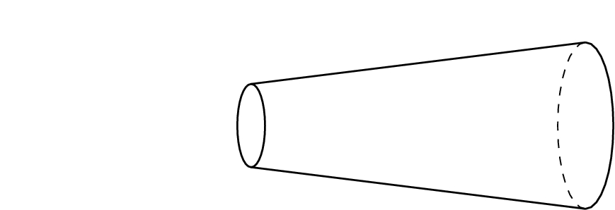
Consider now a small parameter $ε > 0$ (throughout this material we shall always have $ε ⩽ 1$ ). Suppose that the fluid flows through a simply connected, thin domain $Ω_{ε}$ of the form $Ω_{ε} = {(x_{1}, x_{2}, x_{3}) \in R^{3} ∣ x_{1} \in (0, 1), (x_{2}, x_{3}) \in ε S (x_{1})},$ where $S (x_{1})$ are sufficiently regular domains – we also suppose the application $x_{1} \mapsto S (x_{1})$ is also smooth enough ( $C^{2}$ regularity is sufficient). For the sake of simplicity we are going to assume $Ω_{ε} \subset D_{ε} = [0, 1] \times [0, ε] \times [0, ε]$ – and the three-part boundary of $Ω_{ε}$ is given by the following: $\begin{array}{l} Γ_{ε} = {(x_{1}, x_{2}, x_{3}) \in R^{3} ∣ x_{1} \in (0, 1), (x_{2}, x_{3}) \in ε \partial S (x_{1})}, \\ Σ_{0}^{ε} = ε S (0), Σ_{1}^{ε} = ε S (1) \end{array}$ (see Fig. 1). Moreover, we suppose that $Σ_{0}^{ε}$ and $Σ_{1}^{ε}$ are perpendicular on $e_{1} = (1, 0, 0)$ .

Fig. 1.

Thin, anisotropic domain.

We make the conventions $Ω_{1} = Ω$ , $Γ_{1} = Γ$ , $Σ_{i}^{1} = Σ_{i}$ . With respect to the boundary conditions, we impose $\{\begin{matrix} u = 0 & on Γ_{ε}, \\ u \times n = 0 & on Σ_{0}^{ε} \cup Σ_{1}^{ε}, \\ p = p^{i} & on Σ_{i}^{ε} \end{matrix}$ (2) with $p^{0}, p^{1} > 0$ given constants. Note that the second condition is equivalent to $u_{2} = u_{3} = 0$ on $Σ_{0}^{ε} \cup Σ_{1}^{ε}$ .

In the next section we prove the existence of the solution using a classical approximation technique, while in the final section we derive a complete asymptotic expansion with respect to the small parameter ε.

2. The existence theorem

The proof of the existence of the solution is based on classical compactness and monotony arguments, and is very similar to the one in [5]. There are two main differences; the first one is that we use different boundary conditions, the importance of which shall become apparent when discussing the asymptotic expansion. On the other hand, there is the problem of controlling the inertial term. While the author of [5] uses a specific property of the viscosity function, we shall use the smallness of ε together with some sharp Poincaré and Sobolev type of inequalities for thin domains.

We call the system given by (1) and (2) problem (P). We say that $(u, p)$ is a solution of (P) if it satisfies (1) in the sense of distributions and (2) in the sense of traces.

We will suppose that $η : R_{+} \to R$ is a function satisfying the following properties: $\begin{array}{l} η \in C (R_{+}), & (3) \\ 0 < η_{0} ⩽ η (x) ⩽ η_{1} \forall x \in R_{+}, & (4) \\ (η (x^{2}) x - η (y^{2}) y) (x - y) ⩾ 0 \forall x, y \in R_{+} . & (5) \end{array}$ Let us note that (5) is equivalent to the fact that the mapping $x \mapsto η (x^{2}) x$ is increasing. In particular, this is true if η is differentiable and $\frac{d}{d x} (η (x^{2}) x) ⩾ 0 \forall x \in R_{+} .$ (6) In order to introduce the variational problem, let us consider the space $V = {v \in H^{1} {(Ω_{ε})}^{3} | div v = 0, v = 0 on Γ_{ε}, v \times n = 0 on Σ_{0}^{ε} \cup Σ_{1}^{ε}} .$ We will say that $u \in V$ is the solution of the variational problem henceforth denoted ( $PV$ ) if it satisfies $\int_{Ω_{ε}} (u \cdot \nabla) u \cdot v + 2 \int_{Ω_{ε}} η (I (u)) D_{i j} (u) D_{i j} (v) + p^{0} \int_{Σ_{0}^{ε}} v \cdot n + p^{1} \int_{Σ_{1}^{ε}} v \cdot n = 0 \forall v \in V$ (7) (we are systematically going to use Einstein’s summation convention). Consider now the space $X = {v \in {(H^{1} (Ω_{ε}))}^{3} | v = 0 on Γ_{ε}, v \times n = 0 on Σ_{0}^{ε} \cup Σ_{1}^{ε}} .$ Define the application $L : X \to X^{'}$ by $⟨ L (u), h ⟩ = \int_{Ω_{ε}} (u \cdot \nabla) u \cdot h + 2 \int_{Ω_{ε}} η (I (u)) D_{i j} (u) D_{i j} (h)$ and $F : X \to R$ by $⟨ F, h ⟩ = - p^{0} \int_{Σ_{0}^{ε}} h \cdot n - p^{1} \int_{Σ_{1}^{ε}} h \cdot n,$ where $⟨ \cdot, \cdot ⟩$ represents the duality between $X^{'}$ and X. It is clear that L is well defined and $F \in X^{'}$ . The problem ( $PV$ ) can be rewritten as: find $u \in V$ such that $⟨ L (u) - F, v ⟩ = 0 \forall v \in V .$

It is a simple matter to verify that if $(u, p)$ is a smooth solution of (P) then u is a solution of ( $PV$ ). Conversely, the following is true.

Proposition 1.

Let u be a solution of ( $PV$ ). Then there exists $p \in L^{2} (Ω_{ε})$ such that $(u, p)$ satisfy (1) in the sense of distributions and (2) in the sense of traces.

Proof.

Let W be the complement of V in X. The proof of the theorem relies on the following lemma. Lemma 1.

The operator $div : W \to L^{2} (Ω_{ε})$ is an isomorphism. Consequently, so is the adjoint ${div}^{*} : L^{2} (Ω_{ε}) \to W^{'}$ .

Proof.

The one-to-one part is clear. To prove the that it is also onto, let $f \in L^{2} (Ω_{ε})$ . Then if $g = f - \frac{1}{| Ω_{ε} |} \int_{Ω_{ε}} f,$ we have $\int_{Ω_{ε}} g = 0$ and so by a well-known result (see [1]) we find there is $u \in {(H_{0}^{1} (Ω_{ε}))}^{3} \subset X$ such that $div u = g$ . Pick now any $h = (h_{1}, 0, 0) \in {(H^{1} (Ω_{ε}))}^{3}$ with $h_{1} = 0 on Γ_{ε}, \int_{\partial Ω_{ε}} h \cdot n = 1 .$ Then $h \in X$ and we get $\int_{Ω_{ε}} (div h - \frac{1}{| Ω_{ε} |}) = 0,$ so by the above mentioned result we obtain a $v \in X$ with $div v = div h - \frac{1}{| Ω_{ε} |}$ . Combining the results we can write $div ψ = f$ where $ψ = u + (h - v) \int_{Ω_{ε}} f \in X$ . Hence if $ψ = ψ_{w} + ψ_{v}$ ( $ψ_{w} \in W$ , $ψ_{v} \in V$ ) is the decomposition of ψ in X then we have found $ψ_{w} \in W$ such that $div ψ_{w} = f$ . □

Returning to the proof of Theorem 1, consider T be the restriction of $L (u) - F$ to W. Clearly $T \in W^{'}$ and so by Lemma 1 there is $p \in L^{2} (Ω_{ε})$ with ${div}^{*} p = T$ . Let $h \in X$ with the decomposition $h = v + w$ with $v \in V$ , $w \in W$ . $⟨ L (u) - F, h ⟩ = ⟨ T, w ⟩ = ⟨ {div}^{*} p, w ⟩ = \int_{Ω_{ε}} p div w = \int_{Ω_{ε}} p div h .$ By taking in the above equation $h \in {(C_{0}^{\infty} (Ω_{ε}))}^{3}$ we get readily that u satisfies the first equation of (1) in the sense of distributions. □

Henceforth, $∥ \cdot ∥$ will always mean the $L^{2}$ norm on $Ω_{ε}$ unless otherwise specified. In virtue of a Poincaré inequality – see further Lemma 4 – it follows that $∥ \nabla u ∥$ is a norm on V equivalent to the $H^{1}$ norm – and from now on we will consider V endowed with this norm.

A simple calculation – integrating twice by parts – shows that if $u \in X = {v \in {(C^{2} (\overline{Ω_{ε}}))}^{3} ∣ v = 0 on Γ_{ε}, v \times n = 0 on Σ_{0}^{ε} \cup Σ_{1}^{ε}}$ then $\int_{Ω_{ε}} \partial_{x_{i}} u_{j} \partial_{x_{j}} u_{i} = \int_{Ω_{ε}} {(div u)}^{2} .$ Since $X$ is dense in X it follows that for all $u \in V$ $\int_{Ω_{ε}} \partial_{x_{i}} u_{j} \partial_{x_{j}} u_{i} = 0,$ so we can write $\int_{Ω_{ε}} {(D_{i j} (u))}^{2} = \frac{1}{2} \int_{Ω_{ε}} {(\partial_{x_{i}} u_{j})}^{2} = \frac{∥ \nabla u ∥^{2}}{2} .$

Let us consider the mapping $A : V \to V^{'}$ defined by $⟨ A (u), v ⟩ = 2 \int_{Ω_{ε}} η (I (u)) D_{i j} (u) D_{i j} (v) \forall u, v \in V .$

Lemma 2.

The operator A is continuous and monotone, i.e. satisfies $⟨ A (u) - A (u^{'}), u - u^{'} ⟩ ⩾ 0 \forall u, u^{'} \in V .$

Proof.

First we prove continuity. Let $u_{n} \to u$ in V. Obviously we can choose a subsequence $u_{m}$ such that $I (u_{m}) \to I (u) a.e.$ (8) We can write $\begin{array}{l} | ⟨ A (u_{m}) - A (u), v ⟩ | ⩽ & 2 \int_{Ω_{ε}} | (η (I (u_{m})) - η (I (u))) D_{i j} (u) D_{i j} (v) | \\ + 2 \int_{Ω_{ε}} | η (I (u_{m})) (D_{i j} (u_{m}) - D_{i j} (u)) D_{i j} (v) | . \end{array}$ We look at the two terms separately. We have $2 \int_{Ω_{ε}} | (η (I (u_{m})) - η (I (u))) D_{i j} (u) D_{i j} (v) | ⩽ α_{m} ∥ \nabla v ∥$ (9) with $α_{m} = 6 {(\int_{Ω_{ε}} {(η (I (u_{m})) - η (I (u)))}^{2} I (u))}^{1 / 2} \to 0,$ (10) owing to the continuity and the boundedness of η, (8) and the use of Lebesgue’s dominated convergence theorem. Secondly, $2 \int_{Ω_{ε}} | η (I (u_{m})) (D_{i j} (u_{m}) - D_{i j} (u)) D_{i j} (v) | ⩽ η_{1} ∥ \nabla (u_{m} - u) ∥ ∥ \nabla v ∥ .$ (11) Therefore from (9), (10) and (11) we derive $A (u_{m}) \to A (u) in V^{'} .$ (12) We have actually proven more. From any subsequence $u_{k}$ of $u_{n}$ we can choose a subsequence $u_{m}$ for which (12) holds. Therefore we have $A (u_{n}) \to A (u)$ in $V^{'}$ , showing the continuity of A.

To prove the monotony of A, let us write $\begin{array}{l} ⟨ A (u) - A (u^{'}), u - u^{'} ⟩ = & 2 \int_{Ω_{ε}} [η (I (u)) I (u) + η (I (u^{'})) I (u^{'}) \\ - (η (I (u)) + η (I (u^{'}))) D_{i j} (u) D_{i j} (u^{'})] . \end{array}$ From the elementary Cauchy–Schwarz inequality $D_{i j} (u) D_{i j} (u^{'}) ⩽ \sqrt{I (u) I (u^{'})}$ we deduce $⟨ A (u) - A (u^{'}), u - u^{'} ⟩ ⩾ 2 \int_{Ω_{ε}} (η (I (u)) \sqrt{I (u)} - η (I (u^{'})) \sqrt{I (u^{'})}) (\sqrt{I (u)} - \sqrt{I (u^{'})})$ and the conclusion follows from (5). □

Define now $L_{0} : V \to V^{'}$ by $⟨ L_{0} (u), v ⟩ = \int_{Ω_{ε}} (u \cdot \nabla) u \cdot v \forall v \in V .$

Lemma 3.

If $u_{n} \to u$ weakly in V, then $L_{0} (u_{n}) \to L_{0} (u)$ weakly in $V^{'}$ .

Proof.

Taking into account the compact inclusion of V into ${(L^{4} (Ω_{ε}))}^{3}$ we deduce that we can choose a subsequence $u_{k}$ such that $u_{k} \to u$ strongly in ${(L^{4} (Ω_{ε}))}^{3}$ . Pick any $v \in V$ . We can write $| ⟨ L_{0} (u_{k}) - L_{0} (u), v ⟩ | ⩽ | \int_{Ω_{ε}} ((u_{k} - u) \cdot \nabla) u_{k} \cdot v | + | \int_{Ω_{ε}} (u \cdot \nabla) (u_{k} - u) \cdot v | .$ The second term is convergent to 0 since the mapping $z \mapsto \int_{Ω_{ε}} (u \cdot \nabla) z \cdot v$ is linear continuous on V, while for the first one we can write $| \int_{Ω_{ε}} ((u_{k} - u) \cdot \nabla) u_{k} \cdot v | ⩽ ∥ \nabla u_{k} ∥ ∥ u_{k} - u ∥_{L^{4}} ∥ v ∥_{L^{4}},$ and since $u_{k}$ is bounded being weakly convergent, we obtain that $⟨ L_{0} (u_{k}), v ⟩ \to ⟨ L_{0} (u), v ⟩$ . Reasoning the same as in Lemma 2, we get the desired result. □

We continue with a technical result, that will prove very useful lemma.

Lemma 4.

For any $u \in H^{1} (Ω_{ε})$ such that $u = 0$ on $Γ_{ε}$ in the sense of traces, the following inequalities hold: $\begin{array}{l} ∥ u ∥ ⩽ ε ∥ \nabla u ∥, \\ ∥ u ∥_{L^{4}} ⩽ c_{0} ε^{1 / 4} ∥ \nabla u ∥ \end{array}$ for some $c_{0}$ independent of ε. Moreover, for all $u \in V$ we have $| p^{0} \int_{Σ_{0}^{ε}} u \cdot n + p^{1} \int_{Σ_{1}^{ε}} u \cdot n | ⩽ ε^{2} | p^{1} - p^{0} | ∥ \nabla u ∥ .$

Proof.

The first is a classical Poincaré inequality in thin domains – see, for instance Proposition 2.1 in [8].

For the second part, use Proposition 2.3 in [8] and the first part of this lemma to find that the embedding constant of $L^{6}$ in $H^{1}$ is independent of ε. Let us call this constant c. By the interpolation inequality we obtain $∥ u ∥_{L^{4}} ⩽ ∥ u ∥^{1 / 4} ∥ u ∥_{L^{6}}^{3 / 4} ⩽ c^{3 / 4} ε^{1 / 4} ∥ \nabla u ∥,$ and so the conclusion is attained with $c_{0} = c^{3 / 4}$ .

Lastly, let us consider the scalar function $f : Ω_{ε} \to R$ given by $f (x_{1}, x_{2}, x_{3}) = - (1 - x_{1}) p^{0} - x_{1} p^{1} .$ By Green’s formula, we can write the following $p^{0} \int_{Σ_{0}^{ε}} u \cdot n + p^{1} \int_{Σ_{1}^{ε}} u \cdot n = \int_{Ω_{ε}} div (f u) = \int_{Ω_{ε}} \nabla f \cdot u,$ and since $| \nabla f | = | p^{1} - p^{0} |$ , an application of Cauchy–Schwarz and the first part of this lemma ensures the proof. □

Henceforth, we shall denote by C various constants independent of ε. Theorem 1.

Assume that η satisfies (3)–(5). Provided $ε > 0$ is small enough, there exists a solution u of the variational problem ( $PV$ ) satisfying $∥ \nabla u ∥ ⩽ C ε^{2} .$ (13)

Proof.

Since V is a separable space, let ${z_{1}, z_{2}, \dots}$ dense in V; moreover, let $V_{n}$ be the finite-dimensional subspace generated by ${z_{1}, \dots, z_{n}}$ . We begin by showing the approximate problem: Find $u \in V_{n}$ such that $⟨ L (u), v ⟩ = ⟨ F, v ⟩ \forall v \in V_{n}$ has at least one solution $u_{n} \in V_{n}$ .

Let us consider the applications $P_{n} : V_{n} \to V_{n}$ defined by $(P_{n} (w), v) = ⟨ L (w) - F, v ⟩ \forall w, v \in V_{n} .$ We intend to use the following classical result, whose proof can be found in [4]. Lemma 5.

Let $P : R^{n} \to R^{n}$ a continuous mapping such that, for some $ρ > 0$ , $(P (ξ), ξ) ⩾ 0 \forall ξ such that | ξ | = ρ .$ Then there exists ξ with $| ξ | ⩽ ρ$ such that $P (ξ) = 0$ .

By Lemma 4 we get $\begin{array}{l} | ⟨ L_{0} (w), w ⟩ | = \int_{Ω_{ε}} (w \cdot \nabla) w \cdot w ⩽ C ε^{1 / 2} ∥ \nabla w ∥^{3} ⩽ C ∥ \nabla w ∥^{3}, \\ | ⟨ F, w ⟩ | ⩽ C ε^{2} ∥ \nabla w ∥ . \end{array}$ Also we have $⟨ A (w), w ⟩ = \int_{Ω_{ε}} η (I (w)) I (w) ⩾ \frac{η_{0}}{2} ∥ \nabla w ∥^{2},$ so we obtain $(P_{n} (w), w) ⩾ \frac{η_{0}}{2} ∥ \nabla w ∥^{2} - C ∥ \nabla w ∥^{3} - C ε^{2} ∥ \nabla w ∥ .$ Hence if $ε ⩽ \frac{η_{0}}{4 C}$ , then for $∥ \nabla w ∥ = ρ_{ε} = \frac{η_{0} - \sqrt{η_{0}^{2} - 16 C^{2} ε^{2}}}{4 C}$ $(P_{n} (w), w) ⩾ 0$ , and so we can apply Lemma 5 to find $u_{n} \in V_{n}$ , $∥ \nabla u_{n} ∥ ⩽ ρ_{ε}$ with $P_{n} (u_{n}) = 0$ . Clearly $ρ_{ε}$ is independent of n so we can choose a subsequence still denoted by $u_{n}$ such that $\begin{array}{l} u_{n} \to u weakly in V, \\ u_{n} \to u strongly in L^{4} . \end{array}$ Moreover, we have $∥ \nabla u ∥ ⩽ lim inf ∥ \nabla u_{n} ∥ ⩽ ρ_{ε} = \frac{16 C ε^{2}}{\sqrt{η_{0}^{2} + 4 C^{2} ε^{2}}} ⩽ \frac{16 C}{η_{0}} ε^{2} .$ (14) Clearly $A (u_{n})$ is bounded in $V^{'}$ , hence we can choose another subsequence such that $A (u_{n}) \to χ weakly in V^{'} .$ (15) Let us now fix $n ⩾ 1$ . Then for all $m ⩾ n$ we have $⟨ A (u_{m}), z_{n} ⟩ + ⟨ L_{0} (u_{m}), z_{n} ⟩ = ⟨ F, z_{n} ⟩ .$ By Lemma 3 and (15) we can pass to the limit as $m \to \infty$ to get $⟨ χ, z_{n} ⟩ + ⟨ L_{0} (u), z_{n} ⟩ = ⟨ F, z_{n} ⟩ .$ Since this is true for all n and ${z_{1}, z_{2}, \dots}$ is dense in V, it easily follows $⟨ χ, v ⟩ + ⟨ L_{0} (u), v ⟩ = ⟨ F, v ⟩ \forall v \in V .$ (16) To conclude, it rests to prove $A (u) = χ$ . Since $u_{n}$ is the solution of the approximate problem, we can write $⟨ A (u_{n}), u_{n} ⟩ + ⟨ L_{0} (u_{n}), u_{n} ⟩ = ⟨ F, u_{n} ⟩ .$ Using similar arguments as those in the proof of Lemma 3 we derive $⟨ L_{0} (u_{n}), u_{n} ⟩ \to ⟨ L_{0} (u), u ⟩$ , and so $lim_{n \to \infty} ⟨ A (u_{n}), u_{n} ⟩ = ⟨ F, u ⟩ - ⟨ L_{0} (u), u ⟩ .$ (17) By Lemma 2, we have $⟨ A (u_{n}), u_{n} - v ⟩ ⩾ ⟨ A (v), u_{n} - v ⟩ \forall v \in V .$ Using (17) we can pass to the limit in the above equation to get $⟨ F, u ⟩ - ⟨ χ, v ⟩ ⩾ ⟨ A (v), u - v ⟩ \forall v \in V .$ By taking $v = u$ in (16) we get $⟨ χ, u ⟩ = ⟨ F, u ⟩$ , so that $⟨ χ - A (v), u - v ⟩ ⩾ 0 \forall v \in V,$ which can be further written as $t ⟨ χ - A (u + t v), v ⟩ ⩽ 0 \forall t \in R, v \in V .$ Using the continuity of A, we derive the desired result. □

3. Asymptotic expansion

In what follows, we make the following convention: if $v : Ω_{ε} \to R^{3} (R)$ then we will denote $\tilde{v} : Ω \to R^{3} (R)$ the application defined by $\tilde{v} (x_{1}, x_{2}, x_{3}) = v (x_{1}, ε x_{2}, ε x_{3}) .$ We will denote by $∥ \cdot ∥_{0}$ the $L^{2}$ norm on Ω. Moreover, we will also systematically use the dummy index k to represent either summation for $k \in {2, 3}$ , either the repeated index. We can write $\{\begin{matrix} {\tilde{u}}_{1} \partial_{x_{1}} {\tilde{u}}_{1} + \frac{{\tilde{u}}_{k} \partial_{x_{k}} {\tilde{u}}_{1}}{ε} + \partial_{x_{1}} \tilde{p} = 2 \partial_{x_{1}} (\tilde{η} \partial_{x_{1}} {\tilde{u}}_{1}) + \frac{\partial_{x_{k}} (\tilde{η} (\partial_{x_{1}} {\tilde{u}}_{k} + (\partial_{x_{k}} {\tilde{u}}_{1}) / ε))}{ε}, \\ {\tilde{u}}_{1} \partial_{x_{1}} {\tilde{u}}_{2} + \frac{{\tilde{u}}_{k} \partial_{x_{k}} {\tilde{u}}_{2}}{ε} + \frac{\partial_{x_{2}} \tilde{p}}{ε} = \partial_{x_{1}} (\tilde{η} (\partial_{x_{1}} {\tilde{u}}_{2} + \frac{\partial_{x_{2}} {\tilde{u}}_{1}}{ε})) + \frac{\partial_{x_{k}} (\tilde{η} (\partial_{x_{2}} {\tilde{u}}_{k} + \partial_{x_{k}} {\tilde{u}}_{2}))}{ε^{2}}, \\ {\tilde{u}}_{1} \partial_{x_{1}} {\tilde{u}}_{3} + \frac{{\tilde{u}}_{k} \partial_{x_{k}} {\tilde{u}}_{3}}{ε} + \frac{\partial_{x_{3}} \tilde{p}}{ε} = \partial_{x_{1}} (\tilde{η} (\partial_{x_{1}} {\tilde{u}}_{3} + \frac{\partial_{x_{3}} {\tilde{u}}_{1}}{ε})) + \frac{\partial_{x_{k}} (\tilde{η} (\partial_{x_{k}} {\tilde{u}}_{3} + \partial_{x_{3}} {\tilde{u}}_{k}))}{ε^{2}}, \\ \partial_{x_{1}} {\tilde{u}}_{1} + \frac{\partial_{x_{k}} {\tilde{u}}_{k}}{ε} = 0, \end{matrix}$ with $\tilde{η} = η (I (\tilde{u}))$ . An elementary calculation shows that $∥ \tilde{u} ∥_{0} = \frac{1}{ε} ∥ u ∥ ⩽ ∥ \nabla u ∥ ⩽ C ε^{2} .$ The above estimate, as well as fair intuitions leads us to formally write $\{\begin{matrix} {\tilde{u}}_{1} = ε^{2} {\tilde{u}}_{1}^{0} + ε^{4} {\tilde{u}}_{1}^{1} + \dots + ε^{2 n + 2} {\tilde{u}}_{1}^{n} + \dots, \\ {\tilde{u}}_{k} = ε^{3} {\tilde{u}}_{k}^{0} + ε^{5} {\tilde{u}}_{k}^{1} + \dots + ε^{2 n + 3} {\tilde{u}}_{k}^{n} + \dots \forall k \in {2, 3}, \\ \tilde{p} = {\tilde{p}}^{0} + ε^{2} {\tilde{p}}^{1} + \dots + ε^{2 n} {\tilde{p}}^{n} + \dots, \end{matrix}$ where ${\tilde{u}}_{α}^{m}$ , ${\tilde{p}}^{m}$ are independent of ε for all $m ⩾ 0$ , $α \in {1, 2, 3}$ . The boundary conditions are expected to become $\{\begin{matrix} {\tilde{u}}_{α}^{m} = 0 & on Γ, \forall m ⩾ 0, α \in {1, 2, 3}, \\ {\tilde{u}}_{k}^{m} = 0 & on Σ_{0} \cup Σ_{1}, \forall m ⩾ 0, k \in {2, 3}, \\ {\tilde{p}}^{0} (i) = p^{i} & on Σ_{i}, \\ {\tilde{p}}^{m} (i) = 0 & on Σ_{i}, \forall m ⩾ 1 . \end{matrix}$ (18) Writing (formally) the Taylor expansion of η in 0 and plugging in the above expansion, we arrive at $\tilde{η} = {\tilde{A}}_{0} + ε^{2} {\tilde{A}}_{1} + \dots + ε^{2 n} {\tilde{A}}_{n} + \dots,$ where ${\tilde{A}}_{n}$ depends only on ${\tilde{u}}^{i}$ for $i < n$ . Note ${\tilde{A}}_{0} = η (0) : = η^{0}$ .

Plugging in the expansions and identifying the coefficients of $ε^{- 1}$ in the second equation, of $ε^{0}$ in the first equation and taking (18) into account we get $\partial_{x_{2}} {\tilde{p}}^{0} = \partial_{x_{3}} {\tilde{p}}^{0} = 0$ and $\{\begin{matrix} - η^{0} \partial_{x_{k}}^{2} {\tilde{u}}_{1}^{0} + \partial_{x_{1}} {\tilde{p}}^{0} = 0 & on S (x_{1}), \\ {\tilde{u}}_{1}^{0} = 0 & on \partial S (x_{1}) . \end{matrix}$ (P₁⁰) Observe that we can solve for ${\tilde{u}}_{1}^{0} (x_{1}, x_{k}) = \partial_{x_{1}} {\tilde{p}}^{0} (x_{1}) W (x_{1}, x_{k})$ , where W is the unique solution of the problem $\{\begin{matrix} Δ_{k} \tilde{v} = 1 / η^{0} & on S (x_{1}), \\ \tilde{v} = 0 & on \partial S (x_{1}), \end{matrix}$ where $Δ_{k}$ signifies the Laplacian in two variables – $Δ_{k} = \partial_{x_{2}}^{2} + \partial_{x_{3}}^{2}$ . To find ${\tilde{p}}^{0}$ let us use (a priori) the following compatibility relation $\int_{S (x_{1})} \partial_{x_{1}} {\tilde{u}}_{1}^{0} = 0 .$ (C₀) If we define $β (x_{1}) = \int_{S (x_{1})} W (x_{1}, x_{k})$ then $\begin{array}{l} {\tilde{p}}^{0} (x_{1}) = p^{0} + \frac{p^{1} - p^{0}}{\int_{0}^{1} \frac{d x_{1}}{β (x_{1})}} \int_{0}^{x_{1}} \frac{d y_{1}}{β (y_{1})}, \\ {\tilde{u}}_{1}^{0} (x_{1}, x_{k}) = \frac{p^{1} - p^{0}}{\int_{0}^{1} \frac{d x_{1}}{β (x_{1})}} \cdot \frac{W (x_{1}, x_{k})}{β (x_{1})} . \end{array}$ Due to the imposed regularity requirements, we have ${\tilde{u}}_{1}^{0} \in C^{2} (\overline{Ω})$ and ${\tilde{p}}^{0} \in C^{1} (\overline{Ω})$ . It is easy to check that $({\tilde{u}}_{1}^{0}, {\tilde{p}}^{0})$ satisfy ( P 1 0 ) in the classical sense, and that ${\tilde{u}}_{1}^{0}$ verifies ( C 0 ) for all $x_{1}$ . The key ingredient for that – and a property which we shall further use – is that whenever $\tilde{w} \in C^{1} (\overline{Ω})$ satisfies $\tilde{w} = 0$ on Γ, in virtue of Reynolds’ transport theorem $\int_{S (x_{1})} \partial_{x_{1}} \tilde{w} = \partial_{x_{1}} \int_{S (x_{1})} \tilde{w} \forall x_{1} .$ Moreover, we have ${\tilde{p}}^{0} (i) = p^{i}$ .

To determine all ${\tilde{u}}_{α}^{m}$ we proceed by complete induction. Let $j ⩾ 1$ . Assume we have found (sufficiently) smooth ${\tilde{u}}_{1}^{i}$ such that $\int_{S (x_{1})} \partial_{x_{1}} {\tilde{u}}_{i}^{0} = 0$ for all $i < j$ and ${\tilde{u}}_{k}^{i}$ for all $i < j - 1$ (nothing if $j = 1$ ). We show how to determine ${\tilde{u}}_{1}^{j}$ , ${\tilde{u}}_{k}^{j - 1}$ , ${\tilde{p}}^{j}$ such that $\int_{S (x_{1})} \partial_{x_{1}} {\tilde{u}}_{1}^{j} = 0 .$ (C_j) Again, plugging in the expansion and identifying in the second and third equation the coefficients of $ε^{2 j - 1}$ and in the last one those of $ε^{2 j}$ , together with (18), we obtain $\{\begin{matrix} - η^{0} \partial_{x_{k}}^{2} {\tilde{u}}_{2}^{j - 1} + \partial_{x_{2}} {\tilde{p}}^{j} = {\tilde{f}}_{2}^{j} & on S (x_{1}), \\ - η^{0} \partial_{x_{k}}^{2} {\tilde{u}}_{3}^{j - 1} + \partial_{x_{3}} {\tilde{p}}^{j} = {\tilde{f}}_{3}^{j} & on S (x_{1}), \\ \partial_{x_{k}} {\tilde{u}}_{k}^{j - 1} = - \partial_{x_{1}} {\tilde{u}}_{1}^{j - 1} & on S (x_{1}), \\ {\tilde{u}}_{2}^{j - 1} = {\tilde{u}}_{3}^{j - 1} = 0 & on \partial S (x_{1}), \end{matrix}$ (P_k^j−1) with $\begin{array}{l} {\tilde{f}}_{l}^{j} = & \sum_{i + m = j - 2} \partial_{x_{1}} ({\tilde{A}}_{i} \partial_{x_{1}} {\tilde{u}}_{l}^{m}) + \sum_{\begin{array}{c} i + m = j - 1 \\ i ⩾ 1 \end{array}} (\partial_{x_{1}} ({\tilde{A}}_{i} \partial_{x_{l}} {\tilde{u}}_{1}^{m}) + 2 \partial_{x_{l}} ({\tilde{A}}_{i} \partial_{x_{l}} {\tilde{u}}_{l}^{m})) \\ + \sum_{\begin{array}{c} i + m = j - 1 \\ i ⩾ 1 \end{array}} \partial_{x_{l}} ({\tilde{A}}_{i} \partial_{x_{2}} {\tilde{u}}_{3}^{m} + \partial_{x_{3}} {\tilde{u}}_{2}^{m}) - \sum_{i + m = j - 3} ({\tilde{u}}_{1}^{i} \partial_{x_{1}} {\tilde{u}}_{l}^{m} + {\tilde{u}}_{k}^{i} \partial_{x_{k}} {\tilde{u}}_{l}^{m}) \end{array}$ for $l \in {2, 3}$ . Observe that ${\tilde{f}}_{l}^{j}$ are known, since they depend on terms ${\tilde{u}}_{1}^{i}$ with $i < j$ and ${\tilde{u}}_{k}^{i}$ with $i < j - 1$ – moreover, they are smooth by the induction hypothesis. In virtue of the compatibility $\int_{S (x_{1})} \partial_{x_{1}} {\tilde{u}}_{j - 1}^{0} = 0,$ it follows (see [1]) that the Stokes system has a unique regular solution $({\tilde{u}}_{k}^{j - 1}, {\tilde{p}}^{j})$ that satisfies ( P k j−1 ) in the classical sense. Note that ${\tilde{p}}^{j}$ is determined up to a constant (for every $x_{1}$ ). Hence we can write ${\tilde{p}}^{j} (x_{1}, x_{k}) = {\tilde{q}}^{j} (x_{1}, x_{k}) + {\tilde{r}}^{j} (x_{1}),$ where ${\tilde{q}}^{j}$ is fixed and ${\tilde{r}}^{j}$ is to be determined.

Finally, plugging the expansion in the first equation and identifying the coefficients of $ε^{2 j}$ and using once again (18) we get $\{\begin{matrix} - η^{0} \partial_{x_{k}}^{2} {\tilde{u}}_{1}^{j} = - \partial_{x_{1}} {\tilde{r}}^{j} + {\tilde{f}}_{1}^{j} & on S (x_{1}), \\ {\tilde{u}}_{1}^{j} = 0 & on \partial S (x_{1}), \end{matrix}$ (P₁^j) with $\begin{array}{l} {\tilde{f}}_{1}^{j} = & \sum_{i + m = j - 1} (2 \partial_{x_{1}} ({\tilde{A}}_{i} \partial_{x_{1}} {\tilde{u}}_{1}^{m}) + \partial_{x_{k}} ({\tilde{A}}_{i} \partial_{x_{1}} {\tilde{u}}_{k}^{m})) + \sum_{\begin{array}{c} i + m = j \\ i ⩾ 1 \end{array}} \partial_{x_{k}} ({\tilde{A}}_{i} \partial_{x_{k}} {\tilde{u}}_{1}^{m}) \\ - \sum_{i + m = j - 2} ({\tilde{u}}_{1}^{i} \partial_{x_{1}} {\tilde{u}}_{1}^{m} + {\tilde{u}}_{k}^{i} \partial_{x_{k}} {\tilde{u}}_{1}^{m}) - \partial_{x_{1}} {\tilde{q}}^{j} . \end{array}$ We can separate into two problems $\{\begin{matrix} - Δ_{k} \tilde{v} = \frac{1}{η^{0}} {\tilde{f}}_{1}^{j} & on S (x_{1}), \\ \tilde{v} = 0 & on \partial S (x_{1}) \end{matrix}$ and $\{\begin{matrix} - Δ_{k} \tilde{v} = - \frac{1}{η^{0}} \partial_{x_{1}} {\tilde{r}}^{j} & on S (x_{1}), \\ \tilde{v} = 0 & on \partial S (x_{1}) . \end{matrix}$ The first problem is a homogeneous Dirichlet, and so it has a uniquely determined solution, say ${\tilde{u}}_{1}^{j, 1}$ . Observe that the second problem has the solution ${\tilde{u}}_{1}^{j, 2} = \partial_{x_{1}} {\tilde{r}}^{j} W$ , where W as previously introduced. Note that if $\int_{S (x_{1})} {\tilde{u}}_{1}^{j, 1} = γ (x_{1})$ then we define ${\tilde{r}}^{j} (x_{1}) = C_{1} + \int_{0}^{x_{1}} \frac{C - γ (x)}{β (x)} d x,$ where C, $C_{1}$ can be determined uniquely by the restrictions ${\tilde{r}}^{j} (0) = {\tilde{r}}^{j} (1) = 0$ . Hence we have completely found ${\tilde{u}}_{1}^{j} = {\tilde{u}}_{1}^{j, 1} + {\tilde{u}}_{1}^{j, 2} .$ Again, it is fairly easy to see that ${\tilde{u}}_{1}^{j}$ is regular, satisfies ( P 1 j ) in the classical sense and also the condition ( C j ). This ends the induction step, and thereby we have determined ${\tilde{u}}^{n}$ , ${\tilde{p}}^{n}$ for all $n ⩾ 0$ .

Before we continue, we introduce some terminology. We call Ω perfect near the boundary – or ( $PNB$ ) – if there exists $δ > 0$ such that $S (x_{1}) = S (0)$ for all $x_{1} \in (0, δ)$ and $S (x_{1}) = S (1)$ for all $x_{1} \in (1 - δ, 1)$ . Given Ω a ( $PNB$ ) domain we say that $\tilde{u} \in C (\overline{Ω})$ has the ( $PNB$ ) property if $\tilde{u} (x_{1}, x_{k}) = \tilde{u} (0, x_{k})$ for all $x_{1} \in (0, δ)$ , $x_{k} \in S (0)$ and $\tilde{u} (x_{1}, x_{k}) = \tilde{u} (1, x_{k})$ for all $x_{1} \in (1 - δ, 1)$ , $x_{k} \in S (1)$ . Whenever these terms are 0 we say that $\tilde{u}$ is 0 near the boundary. Obviously, if $\tilde{u} \in C^{m} (\overline{Ω})$ has the ( $PNB$ ) property then all the derivatives up to the order m enjoy the same property; moreover, $\partial_{x_{1}}^{α_{1}} \partial_{x_{k}}^{α_{k}} \tilde{u} = 0$ whenever $α_{1} > 0$ . Finally, it is trivial to see that sum/product of functions with the ( $PNB$ ) property has it also, while if one terms is 0 near the boundary then so is the product.

Lemma 6.

Assume that Ω is ( $PNB$ ). Then $\begin{array}{l} {\tilde{u}}_{k}^{j} (0) = {\tilde{u}}_{k}^{j} (1) \equiv 0 \forall j ⩾ 0, \\ {\tilde{p}}^{j} (0) = {\tilde{p}}^{j} (1) \equiv 0 \forall j ⩾ 1 . \end{array}$

Proof.

We shall prove by induction the following: ${\tilde{u}}_{1}^{j}$ , ${\tilde{u}}_{k}^{j}$ , ${\tilde{q}}^{j}$ have the ( $PNB$ ) property, ${\tilde{u}}_{k}^{j} (0) = {\tilde{u}}_{k}^{j} (1) \equiv 0$ for all $j ⩾ 0$ and ${\tilde{p}}^{j} (0) = {\tilde{p}}^{j} (1) \equiv 0$ $\forall j ⩾ 1$ . Observe that, by definition, ${\tilde{u}}_{1}^{0}$ has the ( $PNB$ ) property. This implies $\partial_{x_{1}} {\tilde{u}}_{1}^{0} = 0$ near the boundary, so that the Stokes system ( P k j−1 ) with $j = 1$ has only trivial solution near the boundary – which completes the first step of induction. Next, assume we have been able to prove the statement for all $i < j$ . Looking at ${\tilde{f}}_{1}^{j}$ , note that it has the ( $PNB$ ) property, being a combination of terms that have the ( $PNB$ ) property – it follows easily that ${\tilde{u}}_{1}^{j}$ has the ( $PNB$ ) property. For ${\tilde{f}}_{k}^{j + 1}$ more can be told – not only does it have the ( $PNB$ ) property, but, since it is a combination of the terms of the form ${\tilde{u}}_{k}^{i}$ and $\partial_{x_{1}} {\tilde{u}}_{α}^{i}$ ( $α \in {1, 2, 3}$ , $i < j$ ) then it is 0 near the boundary – hence the system ( P k j−1 ) (with $j + 1$ in place of j) has only trivial solution near the boundary, thus completing the induction. □

Let $\begin{array}{l} u_{1}^{n} (x_{1}, x_{k}) = \sum_{j = 0}^{n} ε^{2 j + 2} {\tilde{u}}_{1}^{j} (x_{1}, \frac{x_{k}}{ε}), \\ u_{l}^{n} (x_{1}, x_{k}) = \sum_{j = 0}^{n} ε^{2 j + 3} {\tilde{u}}_{k}^{j} (x_{1}, \frac{x_{k}}{ε}), l \in {2, 3}, \\ p^{n} (x_{1}, x_{k}) = \sum_{j = 0}^{n} ε^{2 j} {\tilde{p}}^{j} (x_{1}, \frac{x_{k}}{ε}) . \end{array}$ Observe that, if Ω is ( $PNB$ ), owing to Lemma 6, $u^{n} \in V \cap C^{2} (\overline{Ω_{ε}})$ and $p^{n} \in C^{1} (\overline{Ω_{ε}})$ with $p^{n} (i) = p^{i}$ for all $n ⩾ 0$ . We can now state the main result in this section.

Theorem 2.

Let $n \in N$ be fixed. Suppose that Ω is ( $PNB$ ), η satisfies (3)–(5) and, in addition, $\begin{array}{l} \exists c > 0 such that | η (a) - η (b) | ⩽ c | \sqrt{a} - \sqrt{b} | \forall a, b ⩾ 0, & (19) \\ η \in C^{n + 1} (R_{+}) . & (20) \end{array}$ Then the following estimates hold: $\begin{matrix} ∥ \nabla (u - u^{n}) ∥ ⩽ C ε^{2 n + 4}, \\ ∥ p - p^{n} ∥ ⩽ C ε^{2 n + 3} . \end{matrix}$ (21)

Proof.

In order to simplify the calculations, let us introduce $A (i), u_{1} (i), u_{k} (i) : Ω_{ε} \to R$ for $i ⩽ n$ defined by $\begin{array}{l} A (i) (x_{1}, x_{k}) = ε^{2 i} {\tilde{A}}_{i} (x_{1}, \frac{x_{k}}{ε}), \\ u_{1} (i) (x_{1}, x_{k}) = ε^{2 i + 2} {\tilde{u}}_{1}^{i} (x_{1}, \frac{x_{k}}{ε}), \\ u_{l} (i) (x_{1}, x_{k}) = ε^{2 i + 3} {\tilde{u}}_{l}^{i} (x_{1}, \frac{x_{k}}{ε}), l \in {2, 3} . \end{array}$ Multiplying Eq. ( P 1 j ) by $ε^{2 j}$ and adding for $j \in {0, \dots, n}$ we obtain $\begin{array}{l} \sum_{i + j ⩽ n - 1} (2 \partial_{x_{1}} (A (i) \partial_{x_{1}} u (j)) + \partial_{x_{k}} (A (i) \partial_{x_{1}} u_{k} (j))) + \sum_{i + j ⩽ n} \partial_{x_{k}} (A (i) \partial_{x_{k}} u_{1} (j)) \\ - \sum_{i + j ⩽ n - 2} (u_{1} (i) \partial_{x_{1}} u_{1} (j) + u_{k} (i) \partial_{x_{k}} u_{1} (j)) - \partial_{x_{1}} p^{n} = 0 . \end{array}$ Using (20) we can write the Taylor development (up to the order n, with the Lagrange remainder) of η in 0, and so we derive – properly this time $η (I (u^{n})) = B_{0} + ε^{2} B_{1} + \dots + ε^{2 N} B_{N}$ for some $N > n$ (actually, $N = (2 n + 3) (n + 1)$ ). It is an easy matter to verify that $B_{i} = A_{i}$ for $i ⩽ n$ . If $(u^{n} \cdot \nabla) u^{n} = w^{n}$ and $2 div (η (I (u^{n})) D u^{n}) = t^{n}$ then a simple calculation shows $\begin{array}{l} w_{1}^{n} = \sum_{i, j = 0}^{n} (u_{1} (i) \partial_{x_{1}} u_{1} (j) + u_{k} (i) \partial_{x_{k}} u_{1} (j)), \\ t_{1}^{n} = \sum_{i ⩾ 0, j ⩽ n} (2 \partial_{x_{1}} (B (i) \partial_{x_{1}} u (j)) + \partial_{x_{k}} (B (i) \partial_{x_{1}} u_{k} (j))) + \sum_{i ⩾ 0, j ⩽ n} \partial_{x_{k}} (B (i) \partial_{x_{k}} u_{1} (j)), \end{array}$ and so we have $w_{1}^{n} + \partial_{x_{1}} p^{n} = t_{1}^{n} + R_{1}^{n},$ where the rest is given by $\begin{array}{l} R_{1}^{n} = & \sum_{i + j ⩾ n - 1} (u_{1} (i) \partial_{x_{1}} u_{1} (j) + u_{k} (i) \partial_{x_{k}} u_{1} (j)) - \sum_{\begin{array}{c} i + j > n \\ j ⩽ n \end{array}} \partial_{x_{k}} (B (i) \partial_{x_{k}} u_{1} (j)) \\ - \sum_{\begin{array}{c} i + j ⩾ n \\ j ⩽ n \end{array}} (2 \partial_{x_{1}} (B (i) \partial_{x_{1}} u (j)) + \partial_{x_{k}} (B (i) \partial_{x_{1}} u_{k} (j))) . \end{array}$ Observe that all the terms in the above development contain powers of ε of at least $2 n + 2$ , and since we proved all ${\tilde{u}}_{α}^{m}$ are sufficiently regular (at least $C^{2} (\overline{Ω_{ε}})$ ), we can write $∥ R_{1}^{n} ∥_{L^{\infty} (Ω_{ε})} ⩽ C ε^{2 n + 2}$ . In a completely similar manner it can be proved that for $k \in {2, 3}$ we have $w_{k}^{n} + \partial_{x_{k}} p^{n} = t_{k}^{n} + R_{k}^{n},$ with $∥ R_{k}^{n} ∥_{L^{\infty} (Ω_{ε})} ⩽ C ε^{2 n + 3}$ . Combining the three equations we obtain $(u^{n} \cdot \nabla) u^{n} + \nabla p^{n} = 2 div (η (I (u^{n})) D u^{n}) + R^{n},$ (22) with the rest satisfying ${∥ R^{n} ∥}_{L^{\infty} (Ω_{ε})} ⩽ C ε^{2 n + 2} .$ (23)

Multiplying (22) by a test $v \in V$ and integrating over $Ω_{ε}$ we obtain $\begin{matrix} \int_{Ω_{ε}} (u^{n} \cdot \nabla) u^{n} \cdot v + 2 \int_{Ω_{ε}} η (I (u^{n})) D_{i j} (u^{n}) D_{i j} (v) + p^{0} \int_{Σ_{0}^{ε}} v \cdot n + p^{1} \int_{Σ_{1}^{ε}} v \cdot n \\ = \int_{Ω_{ε}} R^{n} \cdot v \forall v \in V . \end{matrix}$ (24) By taking in (7) and (24) $v = u - v^{n}$ and subtracting the two we get $\begin{matrix} 2 \int_{Ω_{ε}} (η (I (u)) D_{i j} (u) - η (I (u^{n})) D_{i j} (u^{n})) D_{i j} (u - u^{n}) \\ = \int_{Ω_{ε}} ((u^{n} \cdot \nabla) u^{n} - (u \cdot \nabla) u) \cdot (u - u^{n}) - \int_{Ω_{ε}} R^{n} \cdot (u - u^{n}) . \end{matrix}$ (25) Note that $\begin{matrix} | \int_{Ω_{ε}} ((u^{n} - u) \cdot \nabla u^{n}) \cdot (u - u^{n}) | ⩽ C ε^{5 / 2} {∥ \nabla (u^{n} - u) ∥}^{2}, \\ | \int_{Ω_{ε}} (u \cdot \nabla (u^{n} - u)) \cdot (u - u^{n}) | ⩽ C ε^{5 / 2} {∥ \nabla (u^{n} - u) ∥}^{2}, \\ | \int_{Ω_{ε}} R^{n} \cdot (u - u^{n}) | ⩽ C ε^{2 n + 4} ∥ \nabla (u^{n} - u) ∥, \end{matrix}$ using the inequalities in Lemma 4, (13) and the elementary following $\begin{array}{l} ∥ \nabla u^{n} ∥ ⩽ C ε^{2}, \\ \int_{Ω_{ε}} | u | ⩽ C ε ∥ u ∥, \end{array}$ so that if $A_{n}$ is the term on right-hand side in (25) then $| A_{n} | ⩽ \frac{η_{0}}{3} {∥ \nabla (u - u^{n}) ∥}^{2} + C ε^{2 n + 4} ∥ \nabla (u - u^{n}) ∥,$ (26) provided ε is small enough. Again, if $B_{n}$ is the term on the left-hand side in (25) then $B_{n} = 2 \int_{Ω_{ε}} η (I (u)) D_{i j}^{2} (u - u^{n}) - 2 \int_{Ω_{ε}} (η (I (u)) - η (I (u^{n}))) D_{i j} (u^{n}) D_{i j} (u - u^{n}) .$ (27) Using (19) in (27) and taking into account the elementary $∥ D_{i j} (u^{n}) ∥_{L^{\infty}} ⩽ C ε$ , it follows – after a Cauchy–Schwarz that $\begin{array}{l} B_{n} & ⩾ η_{0} {∥ \nabla (u - u^{n}) ∥}^{2} - C ε ∥ \sqrt{I (u)} - \sqrt{I (u^{n})} ∥ ∥ \nabla (u - u^{n}) ∥ \\ ⩾ η_{0} {∥ \nabla (u - u^{n}) ∥}^{2} - C ε {∥ \nabla (u - u^{n}) ∥}^{2} ⩾ \frac{2 η_{0}}{3} {∥ \nabla (u - u^{n}) ∥}^{2} & (28) \end{array}$ for small enough ε – to derive the second part of the above inequality we have used the trivial $| \sqrt{I (u)} - \sqrt{I (u^{n})} | ⩽ \sqrt{\sum_{1 ⩽ i, j ⩽ 3} {(D_{i j} (u - u^{n}))}^{2}} .$ Combining (26) and (28) we get $∥ \nabla (u - u^{n}) ∥ ⩽ C ε^{2 n + 4} .$ (29) In order to obtain the pressure estimate, we are going to use the following result. Lemma 7.

Let $f : Ω_{ε} \to R$ with $f \in L^{2} (Ω_{ε})$ and $\int_{Ω_{ε}} f = 0 .$ Then there exists $ϕ \in {(H_{0}^{1} (Ω_{ε}))}^{3}$ such that $\begin{array}{l} div ϕ = f on Ω_{ε}, \\ ∥ \nabla ϕ ∥ ⩽ C ε^{- 1} ∥ f ∥ . \end{array}$

Proof.

As usual, let $\tilde{f} : Ω \to R$ be given by $\tilde{f} (x_{1}, x_{k}) = f (x_{1}, ε x_{k})$ . Since $\int \tilde{f} = 0$ we can use a classical result (see [1]) to find a $\tilde{ψ} : Ω \to R^{3}$ with $\tilde{ψ} \in {(H_{0}^{1} (Ω))}^{3}$ and $div \tilde{ψ} = \tilde{f}$ . We can now define $ϕ (x_{1}, x_{k}) = ({\tilde{ψ}}_{1} (x_{1}, \frac{x_{k}}{ε}), ε {\tilde{ψ}}_{2} (x_{1}, \frac{x_{k}}{ε}), ε {\tilde{ψ}}_{3} (x_{1}, \frac{x_{k}}{ε})) .$ Clearly $div ϕ = f$ and $ϕ = 0$ on $\partial Ω_{ε}$ . To conclude, let us observe that $∥ \nabla ϕ ∥ ⩽ ∥ \nabla \tilde{ψ} ∥_{0} and ∥ f ∥ = ε ∥ \tilde{f} ∥_{0},$ so that the conclusion is achieved, with the constant explicitly given by $C = \frac{∥ \nabla \tilde{ψ} ∥_{0}}{∥ \tilde{f} ∥_{0}} . □$

Returning to the proof of the theorem, let us note that, since p is defined up to a constant we can choose it such that $\int_{Ω_{ε}} p - p_{n} = 0 .$ From Lemma 7, it follows that there exists $ϕ_{n} \in {(H_{0}^{1} (Ω_{ε}))}^{3}$ such that: $\begin{array}{l} div ϕ_{n} = p - p^{n} on Ω_{ε}, \\ ∥ \nabla ϕ_{n} ∥ ⩽ C ε^{- 1} ∥ p - p^{n} ∥ . \end{array}$ Consider the first equation in (1) – understood in distributional sense – and (22). By subtracting the two and then applying $ϕ_{n} \in {(H_{0}^{1} (Ω_{ε}))}^{3}$ we obtain $\begin{array}{l} ∥ p - p_{n} ∥^{2} + 2 \int_{Ω_{ε}} (η (I (u)) D_{i j} (u) - η (I (u^{n})) D_{i j} (u^{n})) D_{i j} (ϕ_{n}) \\ = \int_{Ω_{ε}} ((u^{n} \cdot \nabla) u^{n} - (u \cdot \nabla) u) \cdot ϕ_{n} - \int_{Ω_{ε}} R^{n} \cdot ϕ_{n} . \end{array}$ Proceeding in a very similar manner to the way we determined the velocity estimates – while also using these estimates – it is easy to establish $∥ p - p_{n} ∥ ⩽ C ε^{2 n + 3} .$ Together with (29), this completes the proof. □

Fig. 2.

Domain without the $(PNB)$ property.

We conclude by making some observations.

Consider the concrete case of a Carreau fluid, whose viscosity law can be expressed as $η_{C} (x) = η_{\infty} + (η_{0} - η_{\infty}) {(1 + λ x)}^{(r - 1) / 2}, λ > 0, 0 < η_{\infty} ⩽ η_{0} .$ Note that condition (20) is verified for all $n \in N$ , while if $r ⩽ 1$ we have $η_{\infty} ⩽ η (x) ⩽ η_{0} \forall x ⩾ 0,$ and, if $φ (x) = η_{C} (x^{2})$ then $| φ^{'} (x) | = (1 - r) λ (η_{0} - η_{\infty}) x {(1 + λ x^{2})}^{(r - 3) / 2} ⩽ \frac{(1 - r) \sqrt{λ} (η_{0} - η_{\infty})}{2},$ which easily implies that (4) and (19) are satisfied. Lastly, if $ψ (x) = x η_{C} (x^{2})$ then $ψ^{'} (x) > (η_{0} - η_{\infty}) {(1 + λ x^{2})}^{(r - 3) / 2} (1 + r λ x^{2}),$ from which follows that, if $r ⩾ 0$ , (5) is also verified. Hence, provided $r \in [0, 1]$ , all the conditions are satisfied, so the results proved can be applied for these types of fluids.

It is easy to see that, if we add (19) to the conditions verified by η in Theorem 1, we can prove that the solution is unique. The proof mimics the one for the velocity estimate in Theorem 2.

The ( $PNB$ ) condition on Ω is sufficient – whether is it necessary or not it is not clear. However, some geometric imposition is definitely required to obtain the desired result. To see this, let us suppose that $S (x_{1}) = (1 + x_{1}) S (0)$ , with $S (0) = D ((\frac{1}{2}, \frac{1}{2}); \frac{1}{4})$ (the open disk centered at $(\frac{1}{2}, \frac{1}{2})$ with radius $1 / 4$ ) – see Fig. 2.

We are going to show that, in spite of the simplicity of the geometry, the estimate (21) does not hold even for $n = 0$ . Assume the contrary. An elementary calculation leads us to ${\tilde{u}}_{1}^{0} (x_{1}, x_{k}) = \frac{4 a {(x_{k} / (1 + x_{1}) - 1 / 2)}^{2} - a / 2}{{(1 + x_{1})}^{2}}$ for some constant $a \neq 0$ so that $\partial_{x_{1}} {\tilde{u}}_{1}^{0} (0, x_{k}) = a (- 12 x_{k}^{2} + 8 x_{k} - \frac{5}{2}) ≢ 0,$ and so the Stokes system ( P k j−1 ), for $j = 1$ and $x_{1} = 0$ , has non-trivial solution. Assume, with no loss of generality, that ${\tilde{u}}_{2}^{0} (0) ≢ 0$ . It is immediate to see that ${∥ \nabla (\tilde{u} - {\tilde{u}}^{0}) ∥}_{0} ⩽ ∥ \nabla (u - u^{0}) ∥ ⩽ C ε^{4},$ and so the trace inequality yields ${∥ {\tilde{u}}_{2} - {\tilde{u}}_{2}^{0} ∥}_{L^{2} (S (0))} ⩽ C ε^{4} .$ But since this holds for all $ε > 0$ and the member on left-hand side and C are independent of ε, it follows that ${\tilde{u}}_{2}^{0} (0) = {\tilde{u}}_{2} (0) \equiv 0$ , which is a contradiction.

References

[1]

G.P.

Galdi, An Introduction to the Mathematical Theory of the Navier–Stokes Equation, 2nd edn, Springer, 2011.

[2]

Gipouloux and

Mariušić-Paloka, Asymptotic Behaviour of the Incompressible Newtonian Flow Through Thin Constricted Fracture, Multiscale Problems in Science and Technology, Springer, 2000.

[3]

O.A.

Ladyzhenskahya, On modification of the Navier–Stokes equations for high velocity gradients, Zap. Nauchn. Sem. LOMI 7 (1968), 126–154.

[4]

J.L.

Lions, Quelques Méthodes de Résolution des Problèmes aux Limites Non Linéaires, Dunod-Gauthier Villars, 1969.

[5]

W.G.

Litvinov, Models for laminar and turbulent flows of viscous and nonlinear viscous fluids, in: Recent Developments in the Theoretical Fluid Mechanics,

G.P.

Galdi and

Necas, eds, Pitman Research Notes in Mathematics Series, Vol. 291, 1992, pp. 78–102.

[6]

Marusic, The asymptotic behaviour of quasi-Newtonian flow through a very thin or a very long curved pipe, Asymptotic Analysis 21 (2001), 73–89.

[7]

J.M.

Sac-Épée and

Taous, On a wide class of nonlinear models for non-Newtonian fluids with mixed boundary conditions in thin domains, Asymptotic Analysis 44 (2005), 151–171.

[8]

Temam and

Ziane, Navier–Stokes equations in three dimensional thin domains with various boundary conditions, Advances in Differential Equations 1(4) (1996), 499–546.