Homogenization of Stokes with Neumann condition on oscillating boundary

Abstract

The stationary Stokes problem in a n-dimensional domain with a rapidly oscillating $(n - 1)$ dimensional boundary prescribed with Neumann boundary condition and periodicity along the lateral sides is considered. We identify the limit equation in a fixed domain with a one dimensional Laplacian-type problem, satisfied on the region covered by the oscillating part of the boundary, coupled with steady Stokes in the complement. The existence and uniqueness of solution for the coupled limit problem is established and, finally, the weak convergences of velocities are improved to strong convergence by introducing corrector terms.

Keywords

Rough boundary unfolding operator boundary homogenization

1. Introduction

In this article we establish a homogenization result for the Stokes system posed in a n-dimensional domain with Neumann boundary condition on the fixed amplitude, rapidly oscillating boundary. Rapid boundary oscillations with small amplitudes for various PDEs have been studied in [1,2,10]. Elliptic problems in domains with Dirichlet condition imposed on the fixed amplitude, rapidly oscillating boundary have been extensively studied in the past decade (cf. [3–5]). The Neumann-type condition on the oscillating boundary for Laplacian has been studied in [8,9,19,22]. The motivation to study the Stokes system comes from our interest to study the fluid-structure interaction problems in which the displacement of the oscillating boundary is governed by equations of elastic structures. Our problem is a step towards getting an insight in to the behaviour of Navier–Stokes system in the oscillating domain and separate the difficulty due to non-linearity. We employ the method of unfolding operator (both interior and boundary) to obtain the homogenization results. The method of unfolding operator is introduced and detailed in [12–14,17].

The article is organized as follows: in Section 2 we introduce the domain with a part of the boundary having rapid oscillations of fixed amplitude. On the oscillating domain we pose the steady state Stokes system with homogeneous Neumann boundary condition on the oscillating part of the boundary. The existence of weak solution to this problem is classical. We obtain uniform estimate for the solutions independent of the oscillating parameter ε. In Section 3, we recall the definition and properties of unfolding operator (both interior and boundary) without proof. The proof for the properties of the unfolding operator is detailed in [18]. In Section 4, we homogenize the Stokes system to obtain the weak formulation of the limit system. We also obtain the limit interface condition between oscillating region and fixed region. Further, we show the existence and uniqueness of the coupled limit system. Finally, we present a corrector-type results for the velocity and pressure convergences.

The results obtained in this article for Stokes system with Neumann boundary condition on the oscillating part agree with that obtained in [9] for the Laplacian problem with Neumann boundary condition. The novelty of the article rests in dealing with the difficulty intrinsic to the Stokes system, viz. pressure convergence and Bogovskii operator in the limit. We obtain the uniform pressure estimates and show the existence and uniqueness of the coupled limit system. The analysis shows that the pressure and incompressibility condition disappear in the region spanned by the oscillating part giving rise to a uni-directional Laplace equation. In contrast to [5], the current work considers the steady Stokes system in a n-dimensional domain with Neumann condition on the oscillating boundary. The result corresponding to [5, Proposition 1] for the Neumann boundary condition (see Theorem 4.1) is not necessarily strong in $H^{1} (Ω)$ . Thus, we establish a corrector result in Theorem 5.1.

2. Problem statement and uniform estimates

In this section we introduce the domain with oscillating boundary and pose the steady Stokes on the domain. We obtain the uniform a priori estimates for both the velocity and pressure. The estimates are obtained as a consequence of suitably modifying the classical argument of Poincaré inequality to obtain a Poincaré constant independent of the oscillating parameter ε.

We adapt the convention of denoting, wherever convenient, a vector $x \in R^{n}$ with n-components as $x = (\hat{x}, x_{n})$ where $\hat{x} = (x_{1}, \dots, x_{n - 1})$ is the first $(n - 1)$ components. Similarly, a n-tuple vector function $v$ is decomposed as $v = (\hat{v}, v_{n})$ where $\hat{v}$ is the first $(n - 1)$ components.

Let $T^{n - 1} : = R^{n - 1} / Z^{n - 1}$ denote the $(n - 1)$ -dimensional torus and let $g : T^{n - 1} \to R$ be a Lipschitz function such that $‖ g ‖_{\infty} < h_{1}$ where $h_{1}, h_{2} \in R$ with $h_{1} < h_{2}$ . 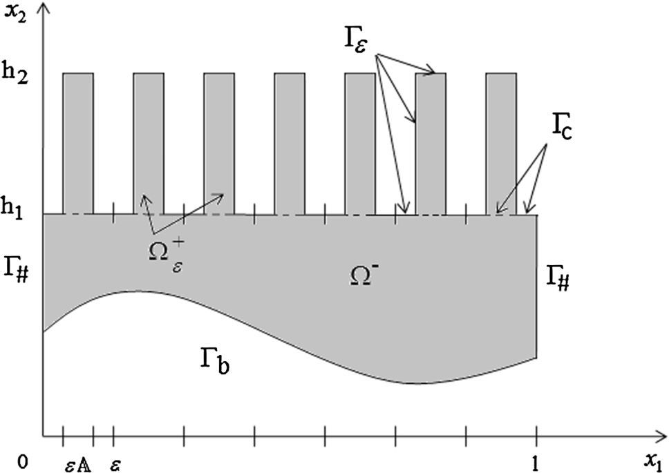Let ${η : [0, 1)}^{n - 1} \to R$ be the step function defined as $\begin{matrix} η (\hat{x}) = \{\begin{matrix} h_{2} & if \hat{x} \in A, \\ h_{1} & {if \hat{x} \in [0, 1)}^{n - 1} ∖ A, \end{matrix} \end{matrix}$ where $A$ is a given proper connected open subset of ${(0, 1)}^{n - 1}$ . Let $θ : = L^{n - 1} (A)$ , the $(n - 1)$ dimensional Lebesgue measure of $A$ . Let $ε > 0$ be a parameter such that $\frac{1}{ε} \in N$ and $N_{ε} : = {1, 2, \dots, \frac{1}{ε}}$ . Set $A_{ε} = ⋃_{k \in N_{ε}^{n - 1}} (ε A + ε k)$ and define $η_{ε} : T^{n - 1} \to R$ by $η_{ε} (\hat{x}) = η (\frac{\hat{x}}{ε})$ . The oscillating domain $Ω_{ε}$ (see Fig. 1) is defined by $\begin{matrix} Ω_{ε} : = {(\hat{x}, x_{n}) \in R^{n} : \hat{x} \in T^{n - 1}, g (\hat{x}) < x_{n} < η_{ε} (\hat{x})} . \end{matrix}$

Fig. 1.

A 2D illustration of $Ω_{ε}$ .

Fig. 2.

A 2D illustration of Ω.

The fixed lower part of the boundary of $Ω_{ε}$ is given by $\begin{matrix} Γ_{b} : = {(\hat{x}, g (\hat{x})) : \hat{x} \in T^{n - 1}} \end{matrix}$ and the oscillating part of the boundary $Γ_{ε} = \partial Ω_{ε} ∖ Γ_{b}$ , where $\partial Ω_{ε}$ denotes boundary of the domain $Ω_{ε}$ . The oscillating (pillar) region of $Ω_{ε}$ is denoted by $Ω_{ε}^{+}$ and is defined by $Ω_{ε}^{+} : = A_{ε} \times (h_{1}, h_{2})$ . Let $Ω^{-}$ denote the region unaffected by boundary oscillations and is defined by $\begin{matrix} Ω^{-} : = {(\hat{x}, x_{n}) : \hat{x} \in T^{n - 1}, g (\hat{x}) < x_{n} < h_{1}} . \end{matrix}$ Let $Γ_{c} : = {(\hat{x}, h_{1}) : \hat{x} \in T^{n - 1}}$ denote the interface between $Ω^{-}$ and $\begin{matrix} Ω^{+} : = {(\hat{x}, x_{n}) : \hat{x} \in T^{n - 1}, h_{1} < x_{n} < h_{2}}, \end{matrix}$ the region where boundary oscillations occur. The upper boundary of $Ω^{+}$ is denoted by $Γ_{u} : = {(\hat{x}, h_{2}) : \hat{x} \in T^{n - 1}}$ . The limit domain with no boundary oscillations, where we expect the limit problem to be posed is defined by (see Fig. 2) $\begin{matrix} Ω : = {(\hat{x}, x_{n}) : 0 < \hat{x} < 1, g (\hat{x}) < x_{n} < h_{2}} . \end{matrix}$

We adapt the convention that for any function space X, the bold font of the same symbol $X$ will denote the vector valued function space $X^{n}$ . For instance, $L^{2} (Ω) : = {[L^{2} (Ω)]}^{n}$ .

For any given $f \in L^{2} (Ω)$ , we propose to study the limit, as $ε \to 0$ , of the steady state Stokes system with Neumann boundary condition on the oscillating part and Dirichlet condition on the fixed boundary: $\begin{matrix} (2.1) & \{\begin{matrix} - Δ u_{ε} + \nabla p_{ε} = f & in Ω_{ε}, \\ div (u_{ε}) = 0 & in Ω_{ε}, \\ \frac{\partial u_{ε}}{\partial ν} - p_{ε} ν = 0 & on Γ_{ε}, \\ u_{ε} = 0 & on Γ_{b} . \end{matrix} \end{matrix}$ Note that the periodicity condition in the $(n - 1)$ -variable has been imposed owing to the condition that $\hat{x}$ belongs to the $(n - 1)$ -dimensional torus. Let $\begin{matrix} C_{Γ_{b}}^{\infty} (\overline{Ω_{ε}}) : = {ϕ \in C^{\infty} ({\overline{Ω}}_{ε}) : ϕ |_{Γ_{b}} = 0} \end{matrix}$ and $H_{Γ_{b}}^{1} (Ω_{ε})$ be the closure of $C_{Γ_{b}}^{\infty} ({\overline{Ω}}_{ε})$ with respect to the $H^{1}$ -norm.

Definition 2.1.

We say a pair $(u_{ε}, p_{ε})$ is a weak solution to (2.1) if, for all $v \in H_{Γ_{b}}^{1} (Ω_{ε})$ , $\begin{matrix} (2.2) & \int_{Ω_{ε}} \nabla u_{ε} : \nabla v d x - \int_{Ω_{ε}} p_{ε} div (v) d x = \int_{Ω_{ε}} f \cdot v d x \end{matrix}$ and, for all $w \in L^{2} (Ω_{ε})$ , $\begin{matrix} (2.3) & \int_{Ω_{ε}} div (u_{ε}) w d x = 0, \end{matrix}$

It is known that there is a unique pair $(u_{ε}, p_{ε}) \in H_{Γ_{b}}^{1} (Ω_{ε}) \times L^{2} (Ω_{ε})$ satisfying (2.2) and (2.3) (cf. [7, Theorem IV.7.1]). Observe that the pressure $p_{ε}$ is unique, as well, owing to the Neumann-type condition on a part of the boundary. Also, there exists a constant $C (Ω_{ε}) > 0$ such that $\begin{matrix} (2.4) & ‖ u_{ε} ‖_{H^{1} (Ω_{ε})} + ‖ p_{ε} ‖_{L^{2} (Ω_{ε})} ⩽ C (Ω_{ε}) ‖ f ‖_{L^{2} (Ω)} . \end{matrix}$ As indicated, the constant $C (Ω_{ε})$ obtained in the above estimate depends on the oscillating parameter ε. However, we wish to obtain an uniform estimate independent of ε in (2.4). Towards this aim, we first modify the argument for Poincaré inequality to suit our context in the following lemma.

Lemma 2.2 (Poincaré inequality).

There exists a constant 1

¹
The symbol C is used for a generic constant, independent of ε, and is not necessarily the same constant everywhere.

C > 0

, depending on

h_{2}

and g but independent of ε, such that

\begin{matrix} ‖ v ‖_{L^{2} (Ω_{ε})} ⩽ C ‖ \nabla v ‖_{L^{2} (Ω_{ε})} \forall v \in H_{Γ_{b}}^{1} (Ω_{ε}) . \end{matrix}

Proof.

The proof is similar to the classical proof of Poincaré inequality, i.e., to integrate along the $x_{n}$ direction. We only highlight here the appropriate changes, in our context, to the classical proof. Similar generalizations for different problem can be found in [11]. Note that it is enough to prove the result for functions in $C_{Γ_{b}}^{\infty} ({\overline{Ω}}_{ε})$ due to its density in $H_{Γ_{b}}^{1} (Ω_{ε})$ with respect to $H^{1}$ norm. Let $ϕ \in C_{Γ_{b}}^{\infty} ({\overline{Ω}}_{ε})$ . Then, for each fixed $\hat{x} \in T^{n - 1}$ , $\begin{matrix} ϕ (\hat{x}, x_{n}) = \int_{g (\hat{x})}^{x_{n}} \frac{\partial ϕ}{\partial x_{n}} (\hat{x}, t) d t ⩽ {(\int_{g (\hat{x})}^{x_{n}} {| \frac{\partial ϕ}{\partial x_{n}} (\hat{x}, x_{n}) |}^{2} d t)}^{1 / 2} {| x_{n} - g (\hat{x}) |}^{1 / 2} . \end{matrix}$ Therefore, $\begin{array}{rcl} (2.5) & {| ϕ (\hat{x}, x_{n}) |}^{2} & ⩽ & \{\begin{matrix} C (\int_{g (\hat{x})}^{h_{2}} | \frac{\partial ϕ}{\partial x_{n}} (\hat{x}, t) |^{2} d t) & if \hat{x} \in A_{ε}, \\ C (\int_{g (\hat{x})}^{h_{1}} | \frac{\partial ϕ}{\partial x_{n}} (\hat{x}, t) |^{2} d t) & if \hat{x} \in T^{n - 1} ∖ A_{ε}, \end{matrix} \end{array}$ where $C = | h_{2} - {inf}_{\hat{x} \in T^{n - 1}} g (\hat{x}) |$ . Thus, $\begin{array}{rcl} ‖ ϕ ‖_{L^{2} (Ω_{ε})}^{2} & = & \int_{A_{ε}} \int_{g (\hat{x})}^{h_{2}} | ϕ |^{2} d x_{n} d \hat{x} + \int_{T^{n - 1} ∖ A_{ε}} \int_{g (\hat{x})}^{h_{1}} | ϕ |^{2} d x_{n} d \hat{x} \\ ⩽ & C^{2} (\int_{A_{ε}} \int_{g (\hat{x})}^{h_{2}} {| \frac{\partial ϕ}{\partial x_{n}} (\hat{x}, t) |}^{2} d t d \hat{x} + \int_{T^{n - 1} ∖ A_{ε}} \int_{g (\hat{x})}^{h_{1}} {| \frac{\partial ϕ}{\partial x_{n}} (\hat{x}, t) |}^{2} d t d \hat{x}) \\ = & C^{2} {‖ \frac{\partial ϕ}{\partial x_{n}} ‖}_{L^{2} (Ω_{ε})}^{2} ⩽ C^{2} ‖ \nabla ϕ ‖_{L^{2} (Ω_{ε})}^{2} . \end{array}$ □

We now show that the Bogovskii operator $div : H_{Γ_{b}}^{1} (Ω_{ε}) \to L^{2} (Ω_{ε})$ is surjective and its inverse ${div}^{- 1} : L^{2} (Ω_{ε}) \to H_{Γ_{b}}^{1} (Ω_{ε}) / N (div)$ , where $N (div)$ denotes the null space of the Bogovskii operator, is uniformly bounded. Similar result for the Bogovskii operator on a fixed domain can be found in [23, 2.1.1 Lemma].

Lemma 2.3.

For each $ε > 0$ and $q_{ε} \in L^{2} (Ω_{ε})$ , there exists a $v_{ε} \in H_{Γ_{b}}^{1} (Ω_{ε})$ and a constant $C > 0$ , independent of ε, such that $div (v_{ε}) = q_{ε}$ in $Ω_{ε}$ and $‖ \nabla v_{ε} ‖_{{[L^{2} (Ω_{ε})]}^{n}} ⩽ C (Ω) ‖ q_{ε} ‖_{L^{2} (Ω_{ε})}$ .

Proof.

We argue along the lines of [15, Lemma 5.1]. Let us extend $q_{ε} \in L^{2} (Ω_{ε})$ to Ω by ${\overline{q}}_{ε}$ defined as $\begin{matrix} {\overline{q}}_{ε} (x) = \{\begin{matrix} q_{ε} & if x \in Ω_{ε}, \\ - \frac{1}{L^{n} (Ω ∖ Ω_{ε})} \int_{Ω_{ε}} q_{ε} d x & if x \in Ω ∖ Ω_{ε}, \end{matrix} \end{matrix}$ where $L^{n} (E)$ denotes the n-dimensional Lebesgue measure of a subset $E \subset R^{n}$ . Observe from the definition that $\int_{Ω} {\overline{q}}_{ε} = 0$ . Also, $\begin{matrix} ‖ {\overline{q}}_{ε} ‖_{L^{2} (Ω)}^{2} = ‖ q_{ε} ‖_{L^{2} (Ω_{ε})}^{2} + \frac{1}{L^{n} (Ω ∖ Ω_{ε})} {(\int_{Ω_{ε}} q_{ε} d x)}^{2} . \end{matrix}$ But $\begin{matrix} \int_{Ω_{ε}} q_{ε} d x ⩽ | \int_{Ω_{ε}} q_{ε} d x | ⩽ ‖ q_{ε} ‖_{L^{1} (Ω_{ε})} ⩽ ‖ q_{ε} ‖_{L^{2} (Ω_{ε})} {[L^{n} (Ω_{ε})]}^{1 / 2} . \end{matrix}$ Hence, $\begin{array}{rcl} ‖ {\overline{q}}_{ε} ‖_{L^{2} (Ω)}^{2} & ⩽ & ‖ q_{ε} ‖_{L^{2} (Ω_{ε})}^{2} + \frac{L^{n} (Ω_{ε})}{L^{n} (Ω ∖ Ω_{ε})} ‖ q_{ε} ‖_{L^{2} (Ω_{ε})}^{2} \\ = & (1 + \frac{L^{n} (Ω_{ε})}{L^{n} (Ω ∖ Ω_{ε})}) ‖ q_{ε} ‖_{L^{2} (Ω_{ε})}^{2} . \end{array}$ Thus, ${\overline{q}}_{ε} \in L_{0}^{2} (Ω)$ . Hence, there is a ${\overline{v}}_{ε} \in H_{0}^{1} (Ω)$ and a constant $C > 0$ , depending on Ω and independent of ε, such that $div ({\overline{v}}_{ε}) = {\overline{q}}_{ε}$ in Ω and $‖ \nabla {\overline{v}}_{ε} ‖_{{[L^{2} (Ω)]}^{n}} ⩽ C ‖ {\overline{q}}_{ε} ‖_{L^{2} (Ω)}$ (see [23, 2.1.1 Lemma]). Let $v_{ε} : = {\overline{v}}_{ε} |_{Ω_{ε}}$ be the restriction of ${\overline{v}}_{ε}$ to $Ω_{ε}$ . Then $\frac{\partial {\overline{v}}_{ε}}{\partial x_{i}} = \frac{\partial v_{ε}}{\partial x_{i}}$ on $Ω_{ε}$ for all $1 ⩽ j ⩽ n$ , in the sense of distributions. Therefore, $‖ v_{ε} ‖_{H_{Γ_{b}}^{1} (Ω_{ε})} ⩽ ‖ {\overline{v}}_{ε} ‖_{H_{0}^{1} (Ω)}$ and $v_{ε} \in H_{Γ_{b}}^{1} (Ω_{ε})$ . Now, for any $ϕ \in C_{c}^{\infty} (Ω_{ε})$ with $\tilde{ϕ}$ being its extension to Ω by zero, $\begin{array}{rcl} \int_{Ω_{ε}} q_{ε} ϕ d x & = & \int_{Ω} {\overline{q}}_{ε} \tilde{ϕ} d x \\ = & \int_{Ω} div ({\overline{v}}_{ε}) \tilde{ϕ} d x \\ = & - \int_{Ω} {\overline{v}}_{ε} \cdot \nabla \tilde{ϕ} d x \\ = & - \int_{Ω_{ε}} v_{ε} \cdot \nabla ϕ d x \\ = & \int_{Ω_{ε}} div (v_{ε}) ϕ d x . \end{array}$ Thus, $div (v_{ε}) = q_{ε}$ in $Ω_{ε}$ , in the sense of distributions. Further, $\begin{array}{rcl} ‖ \nabla v_{ε} ‖_{{[L^{2} (Ω_{ε})]}^{n}} & ⩽ & ‖ \nabla {\overline{v}}_{ε} ‖_{{[L^{2} (Ω)]}^{n}} \\ ⩽ & C ‖ {\overline{q}}_{ε} ‖_{L^{2} (Ω)} \\ ⩽ & C {(1 + \frac{L^{n} (Ω_{ε})}{L^{n} (Ω ∖ Ω_{ε})})}^{1 / 2} ‖ q_{ε} ‖_{L^{2} (Ω_{ε})} . \end{array}$ Since $L^{n} (Ω_{ε}^{+}) = (h_{2} - h_{1}) L^{n - 1} (A_{ε}) = (h_{2} - h_{1}) θ$ and $L^{n} (Ω ∖ Ω_{ε}) = L^{n} (Ω^{+} ∖ Ω_{ε}^{+}) = (h_{2} - h_{1}) (1 - θ)$ , we have a constant independent of ε. □

We now have enough tools to obtain an uniform estimate on both the velocity and pressure.

Theorem 2.4.

Let $f \in L^{2} (Ω)$ and $ε > 0$ . If $(u_{ε}, p_{ε}) \in H_{Γ_{b}}^{1} (Ω_{ε}) \times L^{2} (Ω_{ε})$ is a weak solution of ( 2.1 ) then both the sequences $‖ u_{ε} ‖_{H^{1} (Ω_{ε})}$ and $‖ p_{ε} ‖_{L^{2} (Ω_{ε})}$ are uniformly (independent of ε) bounded.

Proof.

Using (2.3), with $w = p_{ε}$ , in (2.2) with $v = u_{ε}$ we obtain $\begin{matrix} ‖ \nabla u_{ε} ‖_{{[L^{2} (Ω_{ε})]}^{n}}^{2} ⩽ ‖ f ‖_{L^{2} (Ω)} ‖ u_{ε} ‖_{L^{2} (Ω_{ε})} . \end{matrix}$ Now, using the Poincaré inequality established in Lemma 2.2 we get $\begin{matrix} ‖ \nabla u_{ε} ‖_{{(L^{2} (Ω_{ε}))}^{n}} ⩽ C ‖ f ‖_{L^{2} (Ω)} . \end{matrix}$ Thus, $‖ u_{ε} ‖_{H_{Γ_{b}}^{1} (Ω_{ε})}$ is uniformly bounded with respect to ε.

Let $v_{ε} \in H_{Γ_{b}}^{1} (Ω_{ε})$ be the pre-image of $p_{ε} \in L^{2} (Ω_{ε})$ corresponding to the Bogovskii operator. Its existence is guaranteed by Lemma 2.3. Now, choosing $v = v_{ε}$ in (2.2), we obtain $\begin{array}{rcl} ‖ p_{ε} ‖_{L^{2} (Ω_{ε})}^{2} & = & \int_{Ω_{ε}} \nabla u_{ε} : \nabla v_{ε} d x - \int_{Ω_{ε}} f \cdot v_{ε} d x \\ ⩽ & ‖ \nabla u_{ε} ‖_{{[L^{2} (Ω_{ε})]}^{n}} ‖ \nabla v_{ε} ‖_{{[L^{2} (Ω_{ε})]}^{n}} + ‖ f ‖_{L^{2} (Ω)} ‖ v_{ε} ‖_{L^{2} (Ω_{ε})} \\ ⩽ & (‖ \nabla u_{ε} ‖_{{[L^{2} (Ω_{ε})]}^{n}} + C ‖ f ‖_{L^{2} (Ω)}) ‖ \nabla v_{ε} ‖_{{[L^{2} (Ω_{ε})]}^{n}} . \end{array}$ The last inequality is a consequence of the Poincaré inequality obtained in Lemma 2.2. Now, using the estimate obtained in Lemma 2.3 and the uniform bound of $‖ \nabla u_{ε} ‖_{{[L^{2} (Ω_{ε})]}^{n}}$ , we conclude that $\begin{matrix} ‖ p_{ε} ‖_{L^{2} (Ω_{ε})}^{2} ⩽ C {(1 + \frac{L^{n} (Ω_{ε})}{L^{n} (Ω ∖ Ω_{ε})})}^{1 / 2} ‖ p_{ε} ‖_{L^{2} (Ω_{ε})} ‖ f ‖_{L^{2} (Ω)} . \end{matrix}$ Therefore, $\begin{matrix} ‖ p_{ε} ‖_{L^{2} (Ω_{ε})} ⩽ C ‖ f ‖_{L^{2} (Ω)} \end{matrix}$ and $‖ p_{ε} ‖_{L^{2} (Ω_{ε})}$ is uniformly bounded. □

3. Periodic unfolding operator

In this section, we recall the method of unfolding operator (both interior and boundary). We employ the unfolding method to obtain the limit problem. The method of unfolding operator is introduced and detailed in [12–14,17]. However, in contrast to earlier works, we have considered the unfolding operator in n-dimensions because the analysis and proofs are not very different.

Let $[\hat{x}]$ denote the vector with integer coordinates, i.e. $[\hat{x}] = (k_{1}, k_{2}, \dots, k_{n - 1})$ such that $k_{i} ⩽ x_{i}$ , for all i. Also, let ${\hat{x}} = \hat{x} - [\hat{x}]$ be the vector with fractional coordinates. Let ${X \to R}$ denote the collection of all real-valued functions with domain X.

Definition 3.1.
The unfolding operator at ε-scale $T^{ε} : {Ω_{ε}^{+} \to R} \to {Ω^{+} \times A \to R}$ is defined by $\begin{matrix} T^{ε} u (\hat{x}, x_{n}, y) = u (ε [\frac{\hat{x}}{ε}] + ε y, x_{n}) . \end{matrix}$ If u is a real-valued functions with domain $Ω^{+}$ then we interpret the unfolding operator acting on u as follows: $T^{ε} (u) = T^{ε} (u |_{Ω_{ε}^{+}})$ . For a vector valued function $u$ , unfolding operator $T^{ε} u$ acts on each component of the vector.

We recall some crucial properties of unfolding operator, for completeness sake. We refer to [12,18] for the details and proofs.
Proposition 3.2.
The unfolding operator $T^{ε}$ has the following properties:
$T^{ε}$ is linear.

$T^{ε}$ is multiplicative, i.e. $T^{ε} (u_{1} u_{2}) = T^{ε} (u_{1}) T^{ε} (u_{2})$ .

Let $u \in L^{1} (Ω_{ε}^{+})$ . Then $\begin{matrix} \int_{Ω^{+} \times A} T^{ε} u d x = \int_{Ω_{ε}^{+}} u d x . \end{matrix}$

Let $u \in H^{1} (Ω_{ε}^{+})$ . Then $\begin{matrix} \frac{\partial}{\partial x_{n}} (T^{ε} u) = T^{ε} (\frac{\partial u}{\partial x_{n}}) and \nabla_{y} (T^{ε} u) = ε T^{ε} (\nabla_{\hat{x}} u) . \end{matrix}$

$‖ T^{ε} u ‖_{L^{2} (Ω^{+} \times A)} = ‖ u ‖_{L^{2} (Ω_{ε}^{+})}$ .

$‖ T^{ε} u ‖_{L^{2} (T^{n - 1}; H^{1} ((h_{1}, h_{2}) \times A))} ⩽ ‖ u ‖_{H^{1} (Ω_{ε}^{+})}$ .

If $u \in L^{2} (Ω^{+})$ then $T^{ε} u \to u$ strongly in $L^{2} (Ω^{+} \times A)$ .

If ${u_{ε}} \subset L^{2} (Ω_{ε}^{+})$ is a sequence such that $T^{ε} u_{ε} ⇀ u$ weakly in $L^{2} (Ω^{+} \times A)$ then $\begin{matrix} {\tilde{u}}_{ε} ⇀ \int_{A} u (\hat{x}, x_{n}, y) d y weakly in L^{2} (Ω^{+}), \end{matrix}$ where ${\tilde{u}}_{ε}$ is the zero extension of $u_{ε}$ to $Ω^{+}$ .

If ${u_{ε}} \subset H^{1} (Ω_{ε}^{+})$ is a sequence such that $T^{ε} u_{ε} ⇀ u$ weakly in $L^{2} (T^{n - 1} \times A; H^{1} (h_{1}, h_{2}))$ then $\begin{matrix} {\tilde{u}}_{ε} ⇀ \int_{A} u (\hat{x}, x_{n}, y) d y weakly in L^{2} (T^{n - 1}; H^{1} (h_{1}, h_{2})) . \end{matrix}$

We now recall the notion of boundary unfolding operator at ε-scale introduced in [18].
Definition 3.3.
The boundary unfolding operator at ε-scale $T_{b}^{ε} : {A_{ε} \to R} \to {T^{n - 1} \times A \to R}$ is defined by $\begin{matrix} T_{b}^{ε} u (\hat{x}, y) = u (ε [\frac{\hat{x}}{ε}] + ε y) . \end{matrix}$

The following properties of boundary unfolding operator is established in [18]. Proposition 3.4.
The boundary unfolding operator $T_{b}^{ε}$ has the following properties:
$T_{b}^{ε}$ is linear.

$T_{b}^{ε}$ is multiplicative, i.e. $T_{b}^{ε} (u_{1} u_{2}) = T_{b}^{ε} (u_{1}) T_{b}^{ε} (u_{2})$ .

Let $u \in L^{2} (A_{ε})$ . Then $T_{b}^{ε} u \in L^{2} (T^{n - 1} \times A)$ .

Let $u \in L^{2} (T^{n - 1})$ , then $T_{b}^{ε} u \to u$ strongly in $L^{2} (T^{n - 1} \times A)$ .

If $u_{ε} \to u$ strongly in $L^{2} (T^{n - 1})$ , then $T_{b}^{ε} u_{ε} \to u$ strongly in $L^{2} (T^{n - 1} \times A)$ .

4. Homogenization

In this section, we obtain the limit problem corresponding to (2.1), in the weak sense, using (2.2) and (2.3). We also prove the existence and uniqueness of the solution of the limit problem. All the main results of this article are accumulated in this section.

We adapt the following notation for restriction and extension: let $v^{+}$ and $v^{-}$ denote the restriction of any function v to $Ω_{ε}^{+}$ or $Ω^{+}$ (clear from the domain of the function) and $Ω^{-}$ , respectively. Also, $\tilde{v}$ will denote the extension of v by zero outside its domain. Let $\begin{matrix} V_{Γ_{b}} (Ω) : = {v \in L^{2} (Ω) : v^{-} \in H^{1} (Ω^{-}), \frac{\partial v}{\partial x_{n}} \in L^{2} (Ω) and v = 0 on Γ_{b}} . \end{matrix}$ The space $V_{Γ_{b}} (Ω)$ will form a Hilbert space with respect to the norm $\begin{matrix} ‖ v ‖_{V_{Γ_{b}} (Ω)}^{2} = {‖ v^{-} ‖}_{H^{1} (Ω^{-})}^{2} + {‖ v^{+} ‖}_{L^{2} (Ω^{+})}^{2} + {‖ \frac{\partial v^{+}}{\partial x_{n}} ‖}_{L^{2} (Ω^{+})}^{2} . \end{matrix}$ If $C_{Γ_{b}}^{\infty} (\overline{Ω}) : = {ψ \in C^{\infty} (\overline{Ω}) : ψ |_{Γ_{b}} = 0}$ then it has been shown in [16, Proposition 4.1] that the space is dense in $V_{Γ_{b}} (Ω)$ with respect to the norm given above. Let $\begin{matrix} V_{σ, Γ_{b}} (Ω) : = {v \in V_{Γ_{b}} (Ω) : div (v^{-}) = 0 on Ω^{-}} . \end{matrix}$ Note that the divergence free condition is satisfied only on the lower part $Ω^{-}$ . It is easy to check that $V_{σ, Γ_{b}} (Ω)$ is a closed subspace of $V_{Γ_{b}} (Ω)$ with respect to the norm in $V_{Γ_{b}} (Ω)$ .

Theorem 4.1.
Let $f \in L^{2} (Ω)$ . If $(u_{ε}, p_{ε})$ is a weak solution of ( 2.1 ) then, up to a subsequence (not relabelled), there exists
$u^{-} \in H^{1} (Ω^{-})$ such that $\begin{matrix} (4.1) & u_{ε}^{-} ⇀ u^{-} in H^{1} (Ω^{-}), \end{matrix}$

$p^{-} \in L^{2} (Ω^{-})$ such that $\begin{matrix} (4.2) & p_{ε}^{-} ⇀ p^{-} in L^{2} (Ω^{-}), \end{matrix}$

and $u^{+} \in L^{2} (T^{n - 1}; H^{1} (h_{1}, h_{2}))$ such that $\begin{array}{l} (4.3a) & \tilde{u_{ε}^{+}} ⇀ θ u^{+} in L^{2} (T^{n - 1}; H^{1} (h_{1}, h_{2})), \\ (4.3b) & \tilde{\frac{\partial u_{ε}^{+}}{\partial x_{j}}} ⇀ \frac{- θ}{n - 1} \frac{\partial u_{n}^{+}}{\partial x_{n}} e_{j} in L^{2} (Ω^{+}) for 1 ⩽ j ⩽ n - 1, \\ (4.3c) & \tilde{\frac{\partial u_{ε}^{+}}{\partial x_{n}}} ⇀ θ \frac{\partial u^{+}}{\partial x_{n}} in L^{2} (Ω^{+}), \\ (4.3d) & \tilde{p_{ε}^{+}} ⇀ \frac{- θ}{n - 1} \frac{\partial u_{n}^{+}}{\partial x_{n}} in L^{2} (Ω^{+}), \end{array}$
where $e_{j} : = (0, \dots, 1, 0, \dots, 0)$ is the n-tuple with 1 in the jth position and 0 elsewhere. Further, the triplet $(u^{+}, u^{-}, p^{-})$ satisfies $\begin{array}{l} θ \int_{Ω^{+}} \frac{\partial \hat{u^{+}}}{\partial x_{n}} \cdot \frac{\partial \hat{v}}{\partial x_{n}} d x + \frac{n θ}{n - 1} \int_{Ω^{+}} \frac{\partial u_{n}^{+}}{\partial x_{n}} \frac{\partial v_{n}}{\partial x_{n}} d x - θ \int_{Ω^{+}} f \cdot v d x \\ (4.4) & = \int_{Ω^{-}} f \cdot v d x + \int_{Ω^{-}} p^{-} div (v) d x - \int_{Ω^{-}} \nabla u^{-} : \nabla v d x, \end{array}$ for all $v \in V_{Γ_{b}} (Ω)$ , and $\begin{matrix} (4.5) & \int_{Ω^{-}} div (u^{-}) w d x = 0, \forall w \in L^{2} (Ω^{-}) . \end{matrix}$
Proof.
By Theorem 2.4, the sequences $u_{ε}^{-}$ and $p_{ε}^{-}$ are bounded in $H^{1} (Ω^{-})$ and $L^{2} (Ω^{-})$ , respectively. Therefore, up to a subsequence, (4.1) and (4.2) are satisfied. Now, using $ϕ \in C_{c}^{\infty} (Ω^{-})$ as a test function in (2.3) and passing to limit, we get $\begin{matrix} \int_{Ω^{-}} div (u_{ε}^{-}) ϕ d x \overset{ε \to 0}{⟶} \int_{Ω^{-}} div (u^{-}) ϕ d x . \end{matrix}$ Thus, we have obtained (4.5) using the density of $C_{c}^{\infty} (Ω^{-})$ in $L^{2} (Ω^{-})$ .

Using the uniform bound of $u_{ε}^{+}$ from Theorem 2.4 in Proposition 3.2(vi) we obtain the uniform bound of $‖ T^{ε} u_{ε}^{+} ‖_{L^{2} (T^{n - 1}; H^{1} ((h_{1}, h_{2}) \times A))}$ . Thus, there exists a $u^{+} \in L^{2} (T^{n - 1}; H^{1} ((h_{1}, h_{2}) \times A))$ such that, for a subsequence, $\begin{matrix} (4.6) & T^{ε} u_{ε}^{+} ⇀ u^{+} weakly in L^{2} (T^{n - 1}; H^{1} ((h_{1}, h_{2}) \times A)) . \end{matrix}$ Thus, $\begin{matrix} \nabla_{y} (T^{ε} u_{ε}^{+}) ⇀ \nabla_{y} u^{+} weakly in {[L^{2} (Ω^{+} \times A)]}^{n - 1} \end{matrix}$ and $\begin{matrix} (\frac{\partial T^{ε} u_{ε}^{+}}{\partial x_{n}}) ⇀ \frac{\partial u^{+}}{\partial x_{n}} in L^{2} (Ω^{+} \times A) . \end{matrix}$ However, using the property of unfolding operator $T^{ε}$ listed in Proposition 3.2(iv), we have $\begin{matrix} ε T^{ε} (\nabla_{\hat{x}} u_{ε}^{+}) ⇀ \nabla_{y} u^{+} weakly in {[L^{2} (Ω^{+} \times A)]}^{n - 1} \end{matrix}$ and $\begin{matrix} (4.7) & T^{ε} (\frac{\partial u_{ε}^{+}}{\partial x_{n}}) ⇀ \frac{\partial u^{+}}{\partial x_{n}} weakly in L^{2} (Ω^{+} \times A) . \end{matrix}$ The first convergence above implies that $\nabla_{y} u^{+} = 0$ , i.e. $u^{+}$ is independent of y-variable. Hence, $u^{+} \in L^{2} (T^{n - 1}; H^{1} (h_{1}, h_{2}))$ . Using the fact that $u^{+}$ is independent of y-variable and the property of unfolding operator $T^{ε}$ listed in Proposition 3.2(ix) in equation (4.6), we establish (4.3a). Again, using the fact that $u^{+}$ is independent of y-variable and the property of unfolding operator $T^{ε}$ listed in Proposition 3.2(viii) in (4.7), we establish (4.3c).

On the other hand, using the uniform bound of $\nabla u_{ε}^{+}$ and $p_{ε}^{+}$ from Theorem 2.4 in Proposition 3.2(v), we obtain the uniform bound of ${T^{ε} \nabla u_{ε}^{+}}$ and ${T^{ε} p_{ε}^{+}}$ in ${[L^{2} (Ω^{+} \times A)]}^{n}$ and $L^{2} (Ω^{+} \times A)$ , respectively. Thus, for a further subsequence, there exists a $Q \in {[L^{2} (Ω^{+} \times A)]}^{n}$ and $q^{+} \in L^{2} (Ω^{+} \times A)$ such that $\begin{array}{l} (4.8) & T^{ε} (\nabla u_{ε}^{+}) ⇀ Q weakly in {[L^{2} (Ω^{+} \times A)]}^{n}, \\ (4.9) & T^{ε} p_{ε}^{+} ⇀ q^{+} weakly in L^{2} (Ω^{+} \times A) . \end{array}$ Comparing (4.7) and (4.8), we conclude that the nth component of Q is $Q_{n} = \frac{\partial u^{+}}{\partial x_{n}}$ . We now wish to identify $Q_{j}$ , for each $1 ⩽ j ⩽ n - 1$ . For each $1 ⩽ j ⩽ n - 1$ and $ϕ \in C_{c}^{\infty} (Ω^{+})$ , define $ψ_{j}^{ε} (x) : = ε ϕ (\hat{x}, x_{n}) {\frac{x_{j}}{ε}}$ . Since the fractional part function is discontinuous only on the integers, $ψ_{j}^{ε}$ is continuous on $Ω_{ε}^{+}$ . Therefore, by the linearity and multiplicative property of unfolding operator (see (i) and (ii) of Proposition 3.2), we obtain $\begin{matrix} T^{ε} (ψ_{j}^{ε}) = ε T^{ε} (ϕ) y_{j} \forall 1 ⩽ j ⩽ n - 1 . \end{matrix}$ Further, by (iv) of Proposition 3.2, we obtain for all $1 ⩽ j ⩽ n - 1$ $\begin{array}{rcl} T^{ε} (\frac{\partial ψ_{j}^{ε}}{\partial x_{i}}) = \{\begin{matrix} \frac{\partial}{\partial x_{n}} T^{ε} (ψ_{j}^{ε}) = ε T^{ε} (\frac{\partial ϕ}{\partial x_{n}}) y_{j} & i = n, \\ \frac{1}{ε} \frac{\partial}{\partial y_{i}} T^{ε} (ψ_{j}^{ε}) = ε T^{ε} (\frac{\partial ϕ}{\partial x_{i}}) y_{j} & i \neq j and 1 ⩽ i ⩽ n - 1, \\ \frac{1}{ε} \frac{\partial}{\partial y_{j}} T^{ε} (ψ_{j}^{ε}) = ε T^{ε} (\frac{\partial ϕ}{\partial x_{j}}) y_{j} + T^{ε} (ϕ) & i = j . \end{matrix} \end{array}$ Therefore, using property (vii) of Proposition 3.2, we obtain the following strong convergences in $L^{2} (Ω^{+} \times A)$ for each $1 ⩽ j ⩽ n - 1$ : $\begin{array}{l} (4.10a) & T^{ε} (ψ_{j}^{ε}) \to 0, \\ (4.10b) & T^{ε} (\nabla ψ_{j}^{ε}) \to ϕ e_{j} . \end{array}$ For a fixed $1 ⩽ i ⩽ n$ and $1 ⩽ j ⩽ n - 1$ , choose $v = ψ_{j}^{ε} e_{i}$ as a test function in (2.2) to obtain $\begin{matrix} \int_{Ω_{ε}^{+}} \nabla u_{ε i}^{+} \cdot \nabla ψ_{j}^{ε} d x - \int_{Ω_{ε}^{+}} p_{ε}^{+} \frac{\partial ψ_{j}^{ε}}{\partial x_{i}} d x = \int_{Ω_{ε}} f_{i} ψ_{j}^{ε} d x, \end{matrix}$ where $u_{ε i}^{+}$ is the ith component of $u_{ε}^{+}$ . Using (ii) and (iii) of Proposition 3.2, we get $\begin{array}{l} \int_{Ω^{+} \times A} T^{ε} (\nabla u_{ε i}^{+}) \cdot T^{ε} (\nabla ψ_{j}^{ε}) d x d y - \int_{Ω^{+} \times A} T^{ε} (p_{ε}^{+}) T^{ε} (\frac{\partial ψ_{j}^{ε}}{\partial x_{i}}) d x d y \\ = \int_{Ω^{+} \times A} T^{ε} (f_{i}) T^{ε} (ψ_{j}^{ε}) d x d y . \end{array}$ Passing to limit, as $ε \to 0$ , and using (4.8), (4.9) and (4.10) we derive that, for all $ϕ \in C_{c}^{\infty} (Ω^{+})$ , $\begin{matrix} \int_{Ω^{+} \times A} Q_{j}^{i} ϕ d x d y = \{\begin{matrix} 0 & i \neq j, \\ \int_{Ω^{+} \times A} q^{+} ϕ d x d y & i = j . \end{matrix} \end{matrix}$ Therefore, for a.e. $x \in Ω^{+}$ , $\begin{matrix} (4.11) & \int_{A} Q_{j}^{i} (x) d y = \{\begin{matrix} 0 & i \neq j, \\ \int_{A} q^{+} (x) d y & i = j . \end{matrix} \end{matrix}$

Using $ϕ \in C_{c}^{\infty} (Ω^{+})$ as a test function in (2.3) and, by (ii) and (iii) of Proposition 3.2, we get $\begin{matrix} \int_{Ω^{+} \times A} T^{ε} (div (u_{ε}^{+})) T^{ε} (ϕ) d x = 0 . \end{matrix}$ By (vii) of Proposition 3.2, $T^{ε} ϕ \to ϕ$ strongly in $L^{2} (Ω^{+} \times A)$ . Therefore, passing to the limit above and using (4.8), we obtain $\begin{matrix} \int_{Ω^{+} \times A} [\sum_{i = 1}^{n - 1} Q_{i}^{i} + \frac{\partial u_{n}^{+}}{\partial x_{n}}] ϕ d x d y = 0 . \end{matrix}$ Since $u^{+}$ is independent of y variable, we have for all $ϕ \in C_{c}^{\infty} (Ω^{+})$ , $\begin{array}{rcl} 0 & = & \int_{Ω^{+}} [\sum_{i = 1}^{n - 1} \int_{A} Q_{i}^{i} d y + θ \frac{\partial u_{n}^{+}}{\partial x_{n}}] ϕ d x \\ = & \int_{Ω^{+}} [(n - 1) \int_{A} q^{+} d y + θ \frac{\partial u_{n}^{+}}{\partial x_{n}}] ϕ d x (By using (4.11)) . \end{array}$ Thus, $\begin{matrix} (4.12) & \int_{A} q^{+} d y = \frac{- θ}{n - 1} \frac{\partial u_{n}^{+}}{\partial x_{n}} a.e. on Ω^{+} . \end{matrix}$ Using Proposition 3.2(viii) in the convergence (4.9) and the identity obtained in (4.12), we establish (4.3d). Similarly, using Proposition 3.2(viii) in the convergence (4.8) and the identity obtained in (4.11) and (4.12), we establish (4.3b).

It now only remains to show (4.4). Let us use $ψ \in C_{Γ_{b}}^{\infty} (\overline{Ω})$ as a test function in (2.2). Then, by (ii) and (iii) of Proposition 3.2, we get $\begin{array}{l} \int_{Ω^{+} \times A} T^{ε} (\nabla u_{ε}^{+}) : T^{ε} (\nabla ψ) d x d y \\ - \int_{Ω^{+} \times A} T^{ε} (p_{ε}^{+}) T^{ε} (div (ψ)) d x d y - \int_{Ω^{+} \times A} T^{ε} (f) \cdot T^{ε} (ψ) d x d y \\ = \int_{Ω^{-}} f \cdot ψ d x + \int_{Ω^{-}} p_{ε}^{-} div (ψ) d x - \int_{Ω^{-}} \nabla u_{ε}^{-} : \nabla ψ d x . \end{array}$ By Proposition 3.2(vii), $T^{ε} f$ , $T^{ε} ψ$ and $T^{ε} (\nabla ψ)$ converge strongly in $L^{2} (Ω^{+} \times A)$ . Thus, using convergences (4.8), (4.9), (4.1) and (4.2), we obtain $\begin{array}{l} \int_{Ω^{+} \times A} Q : \nabla ψ d x d y - \int_{Ω^{+} \times A} q^{+} div (ψ) d x d y - \int_{Ω^{+} \times A} f \cdot ψ d x d y \\ (4.13) & = \int_{Ω^{-}} f \cdot ψ d x + \int_{Ω^{-}} p^{-} div (ψ) d x - \int_{Ω^{-}} \nabla u^{-} : \nabla ψ d x . \end{array}$ Let us now simplify the first two terms on the left hand side of the above equation. $\begin{array}{l} \int_{Ω^{+} \times A} [Q : \nabla ψ - q^{+} div (ψ)] d x d y \\ = \sum_{j = 1}^{n - 1} \int_{Ω^{+} \times A} Q_{j} \cdot \frac{\partial ψ}{\partial x_{j}} d x d y \\ + \int_{Ω^{+} \times A} Q_{n} \cdot \frac{\partial ψ}{\partial x_{n}} d x d y - \sum_{j = 1}^{n} \int_{Ω^{+}} (\int_{A} q^{+} d y) \frac{\partial ψ_{j}}{\partial x_{j}} d x \\ = \sum_{j = 1}^{n - 1} \int_{Ω^{+}} (\int_{A} q^{+} d y) \frac{\partial ψ_{j}}{\partial x_{j}} d x \\ + θ \int_{Ω^{+}} \frac{\partial u^{+}}{\partial x_{n}} \cdot \frac{\partial ψ}{\partial x_{n}} d x - \sum_{j = 1}^{n} \int_{Ω^{+}} (\int_{A} q^{+} d y) \frac{\partial ψ_{j}}{\partial x_{j}} d x \\ = θ \int_{Ω^{+}} \frac{\partial u^{+}}{\partial x_{n}} \cdot \frac{\partial ψ}{\partial x_{n}} d x + \frac{θ}{n - 1} \int_{Ω^{+}} \frac{\partial u_{n}^{+}}{\partial x_{n}} \frac{\partial ψ_{n}}{\partial x_{n}} d x . \end{array}$ The second equality is obtained from (4.11) and the independence of $u^{+}$ in y-variable. The last equality is obtained from (4.12). Using above simplification in (4.13), we establish $\begin{array}{l} θ \int_{Ω^{+}} \frac{\partial u^{+}}{\partial x_{n}} \cdot \frac{\partial ψ}{\partial x_{n}} d x + \frac{θ}{n - 1} \int_{Ω^{+}} \frac{\partial u_{n}^{+}}{\partial x_{n}} \frac{\partial ψ_{n}}{\partial x_{n}} d x - θ \int_{Ω^{+}} f \cdot ψ d x \\ = \int_{Ω^{-}} f \cdot ψ d x + \int_{Ω^{-}} p^{-} div (ψ) d x - \int_{Ω^{-}} \nabla u^{-} : \nabla ψ d x \end{array}$ for all $ψ \in C_{Γ_{b}}^{\infty} (\overline{Ω})$ and by density is true in $V_{Γ_{b}} (Ω)$ . Thus, we have established (4.4). This completes the proof. □
Theorem 4.2.
Let $(u^{+}, u^{-}, p^{-})$ be the triplet obtained in Theorem 4.1 . Let $u$ be defined by $\begin{matrix} u (x) = \{\begin{matrix} u^{+} & if x \in Ω^{+}, \\ u^{-} & if x \in Ω^{-} . \end{matrix} \end{matrix}$ Then $u \in V_{σ, Γ_{b}} (Ω)$ .
Proof.
Note that, by definition, $u \in L^{2} (Ω)$ . By (4.1), the restriction of $u$ to $Ω^{-}$ , i.e. $u^{-}$ , is in $H^{1} (Ω^{-})$ . Also, by the weak continuity of trace operator from $H^{1} (Ω^{-})$ to $H^{1 / 2} (Γ_{b})$ and the convergence (4.1), we obtain $u^{-} |_{Γ_{b}} = 0$ . Also, from (4.5), we have that $div (u^{-}) = 0$ a.e. in $Ω^{-}$ . It now only remains to show that $\frac{\partial u}{\partial x_{n}} \in L^{2} (Ω)$ . But we already have $\frac{\partial u^{-}}{\partial x_{n}} \in L^{2} (Ω^{-})$ and $\frac{\partial u^{+}}{\partial x_{n}} \in L^{2} (Ω^{+})$ . Thus, our claim is achieved if one shows that $u^{+}$ and $u^{-}$ matches on the interface boundary $Γ_{c}$ , in the sense of trace. Let $I_{ε}$ denote the interface of oscillating domain, i.e. $I_{ε} : = A_{ε} \times {h_{1}}$ . We first observe the fact that $u_{ε}^{+} |_{I_{ε}} = u_{ε}^{-} |_{I_{ε}}$ , in the sense of trace. For any $v \in H_{Γ_{b}}^{1} (Ω_{ε})$ and $1 ⩽ i ⩽ n$ , $\begin{array}{rcl} \int_{Ω_{ε}} \frac{\partial u_{ε}}{\partial x_{i}} \cdot v d x & = & - \int_{Ω_{ε}} u_{ε} \cdot \frac{\partial v}{\partial x_{i}} d x + \int_{Γ_{ε}} u_{ε} \cdot v ν_{i} d S \\ = & - \int_{Ω_{ε}^{+}} u_{ε}^{+} \cdot \frac{\partial v}{\partial x_{i}} d x - \int_{Ω^{-}} u_{ε}^{-} \cdot \frac{\partial v}{\partial x_{i}} d x + \int_{Γ_{ε} ∖ Γ_{c}} u_{ε}^{+} \cdot v ν_{i} d S \\ + \int_{Γ_{c} ∖ I_{ε}} u_{ε}^{-} \cdot v ν_{i} d S \\ = & \int_{Ω_{ε}^{+}} \frac{\partial u_{ε}^{+}}{\partial x_{i}} \cdot v d x + \int_{Ω_{ε}^{-}} \frac{\partial u^{-}}{\partial x_{i}} \cdot v d x + \int_{I_{ε}} (u_{ε}^{+} - u_{ε}^{-}) \cdot v d S . \end{array}$ Also, $\begin{array}{rcl} \int_{Ω_{ε}} \frac{\partial u_{ε}}{\partial x_{i}} \cdot v d x & = & \int_{Ω_{ε}^{+}} {(\frac{\partial u_{ε}}{\partial x_{i}})}^{+} \cdot v d x + \int_{Ω^{-}} {(\frac{\partial u_{ε}}{\partial x_{i}})}^{-} \cdot v d x \\ = & \int_{Ω_{ε}^{+}} \frac{\partial u_{ε}^{+}}{\partial x_{i}} \cdot v d x + \int_{Ω_{ε}^{-}} \frac{\partial u^{-}}{\partial x_{i}} \cdot v d x . \end{array}$ The second equality above is a consequence of the fact that ${(\frac{\partial u_{ε}}{\partial x_{i}})}^{+} = \frac{\partial u_{ε}^{+}}{\partial x_{i}}$ and ${(\frac{\partial u_{ε}}{\partial x_{i}})}^{-} = \frac{\partial u_{ε}^{-}}{\partial x_{i}}$ , in the sense of distributions. Thus, $\begin{matrix} \int_{I_{ε}} (u_{ε}^{+} - u_{ε}^{-}) \cdot v d S = 0 . \end{matrix}$ Hence $u_{ε}^{+} = u_{ε}^{-}$ on $I_{ε}$ , in the sense of trace. By the linearity of the boundary unfolding operator, $T_{b}^{ε}$ , we get $\begin{matrix} (4.14) & T_{b}^{ε} (u_{ε}^{+} |_{I_{ε}}) = T_{b}^{ε} (u_{ε}^{-} |_{I_{ε}}) a.e. on Γ_{c} \times A . \end{matrix}$ We wish to pass to the limit, as $ε \to 0$ , on both sides of (4.14). Let us first compute the limit of $T_{b}^{ε} (u_{ε}^{-} |_{I_{ε}})$ on RHS. Using the weak continuity of the trace map on the convergence (4.1), we get $\begin{matrix} u_{ε}^{-} ⇀ u^{-} weakly in H^{1 / 2} (Γ_{c}) \end{matrix}$ and, by the compact imbedding of $H^{1 / 2} (Γ_{c})$ in $L^{2} (Γ_{c})$ , we obtain $\begin{matrix} u_{ε}^{-} \to u^{-} strongly in L^{2} (Γ_{c}) . \end{matrix}$ Thus, by Proposition 3.4(v), we obtain $\begin{matrix} (4.15) & T_{b}^{ε} (u_{ε}^{-} |_{I_{ε}}) \to u^{-} strongly in L^{2} (Γ_{c} \times A) . \end{matrix}$ Now, let us first compute the limit of $T_{b}^{ε} (u_{ε}^{+} |_{I_{ε}})$ on LHS. Note that $T_{b}^{ε} (u_{ε}^{+} |_{I_{ε}}) = (T^{ε} u_{ε}^{+}) |_{Γ_{c} \times A}$ because $(T^{ε} u_{ε}^{+}) |_{Γ_{c} \times A} = u_{ε}^{+} (ε [\frac{\hat{x}}{ε}] + ε y, h_{1}) = T_{b}^{ε} (u_{ε}^{+} |_{I_{ε}})$ on $Γ_{c} \times A$ . Using the weak continuity of the trace map on the convergence (4.6), we get $\begin{matrix} T^{ε} (u_{ε}^{+}) ⇀ u^{+} weakly in L^{2} (T^{n - 1}; H^{1 / 2} (A \times {h_{1}})) \end{matrix}$ and, by the continuous imbedding of $L^{2} (T^{n - 1}; H^{1 / 2} (A \times {h_{1}}))$ in $L^{2} (T^{n - 1}; L^{2} (A \times {h_{1}})) = L^{2} (Γ_{c} \times A)$ , we obtain $\begin{matrix} (4.16) & T^{ε} (u_{ε}^{+}) ⇀ u^{+} weakly in L^{2} (Γ_{c} \times A) . \end{matrix}$ Passing to the limit, $ε \to 0$ , in (4.14) and using the informations (4.15) and (4.16), we obtain $\begin{matrix} u^{+} = u^{-} a.e. in Γ_{c} \times A . \end{matrix}$ Since $u^{+}$ and $u^{-}$ are independent of y-variable, we get $u^{+} = u^{-}$ on $Γ_{c}$ . □

In the following result, we identify the PDE, in the sense of distributions, whose weak formulation is precisely (4.4) and (4.5).
Theorem 4.3.
Let $f \in L^{2} (Ω)$ and $(u, p^{-})$ satisfy the system of equations ( 4.4 ) and ( 4.5 ). If, in addition, the solution $u : Ω \to R^{n}$ is such that $u \in H^{2} (Ω^{-})$ , $\frac{\partial^{i} u}{\partial x_{n}^{i}} \in L^{2} (Ω)$ for $i = 0, 1, 2$ and $p^{-} \in H^{1} (Ω^{-})$ , then $(u, p^{-})$ satisfies the following system of equations pointwise a.e. in Ω: $\begin{array}{l} (4.17a) & \{\begin{matrix} - \frac{\partial^{2} \hat{u^{+}}}{\partial x_{n}^{2}} = \hat{f} & in Ω^{+}, \\ - \frac{\partial^{2} u_{n}^{+}}{\partial x_{n}^{2}} = \frac{n - 1}{n} f_{n} & in Ω^{+}, \\ \frac{\partial u^{+}}{\partial x_{n}} = 0 & on Γ_{u}, \end{matrix} \\ (4.17b) & \{\begin{matrix} - Δ u^{-} + \nabla p^{-} = f & in Ω^{-}, \\ div (u^{-}) = 0 & in Ω^{-}, \\ u^{-} = 0 & on Γ_{b}, \end{matrix} \\ (4.17c) & \{\begin{matrix} u^{+} = u^{-} & on Γ_{c}, \\ θ \frac{\partial \hat{u^{+}}}{\partial x_{n}} = \frac{\partial \hat{u^{-}}}{\partial x_{n}} & on Γ_{c}, \\ \frac{n θ}{n - 1} \frac{\partial u_{n}^{+}}{\partial x_{n}} = \frac{\partial u_{n}^{-}}{\partial x_{n}} - p^{-} & on Γ_{c} . \end{matrix} \end{array}$
Proof.
We prove the result in three steps – one each for the sub-equations of (4.17).
Let us use a $ψ \in C^{\infty} (\overline{Ω})$ such that $ψ = 0$ on $\overline{Ω^{-}}$ as a test function in (4.4) to obtain $\begin{matrix} θ \int_{Ω^{+}} \frac{\partial \hat{u^{+}}}{\partial x_{n}} \cdot \frac{\partial \hat{ψ}}{\partial x_{n}} + \frac{n}{n - 1} θ \int_{Ω^{+}} \frac{\partial u_{n}^{+}}{\partial x_{n}} \frac{\partial ψ_{n}}{\partial x_{n}} = θ \int_{Ω^{+}} f \cdot ψ \end{matrix}$ and, using integration by parts, we get $\begin{array}{l} - \int_{Ω^{+}} \frac{\partial^{2} \hat{u^{+}}}{\partial x_{n}^{2}} \cdot \hat{ψ} d x + \int_{Γ_{u}} \frac{\partial \hat{u^{+}}}{\partial x_{n}} \cdot \hat{ψ} d S - \frac{n}{n - 1} \int_{Ω^{+}} \frac{\partial^{2} u_{n}^{+}}{\partial x_{n}^{2}} ψ_{n} d x \\ + \frac{n}{n - 1} \int_{Γ_{u}} \frac{\partial u_{n}^{+}}{\partial x_{n}} ψ_{n} d S \\ (4.18) & = θ \int_{Ω^{+}} f \cdot ψ d x . \end{array}$ In particular, for any $ψ \in C_{c}^{\infty} (Ω^{+})$ , choosing $ψ = \sum_{i = 1}^{n - 1} ψ e_{i}$ , we get $\begin{matrix} - \int_{Ω^{+}} \frac{\partial^{2} \hat{u^{+}}}{\partial x_{n}^{2}} \cdot \hat{ψ} d x = \int_{Ω^{+}} \hat{f} \cdot \hat{ψ} d x \end{matrix}$ and $ψ = ψ e_{n}$ , we get $\begin{matrix} - \frac{n}{n - 1} \int_{Ω^{+}} \frac{\partial^{2} u_{n}^{+}}{\partial x_{n}^{2}} ψ d x = \int_{Ω^{+}} f_{n} ψ d x . \end{matrix}$ Therefore, by density of $C_{c}^{\infty} (Ω^{+})$ in $L^{2} (Ω^{+})$ we obtain the first two equations of (4.17a). We now check the validity of boundary condition of (4.17a). For any $ψ \in C^{\infty} (\overline{Ω^{+}})$ such that $ψ |_{Γ_{c}} = 0$ and using $ψ = \sum_{i = 1}^{n - 1} ψ e_{i}$ and the first equation of (4.17a) in (4.18), we obtain $\begin{matrix} - \int_{Γ_{u}} \frac{\partial \hat{u^{+}}}{\partial x_{n}} \cdot \hat{ψ} d S = 0 . \end{matrix}$ Similarly, using $ψ = ψ e_{n}$ and the second equation of (4.17a) in (4.18), we obtain $\begin{matrix} \int_{Γ_{u}} \frac{\partial u_{n}^{+}}{\partial x_{n}} ψ d S = 0 . \end{matrix}$ Hence, by a classical result (see [6, Lemma 6.2.1]), we obtain the boundary condition in (4.17a).

From Theorem 4.2, we have $div (u^{-}) = 0$ on $Ω^{-}$ and $u^{-} = 0$ of $Γ_{b}$ . Thus, it only remains to prove the first equation of (4.17b). Let us use $ψ \in C_{c}^{\infty} (Ω)$ which is compactly supported in $Ω^{-}$ as a test function in (4.4) to obtain $\begin{matrix} \int_{Ω^{-}} \nabla u^{-} : \nabla ψ d x - \int_{Ω^{-}} p^{-} div (ψ) d x = \int_{Ω^{-}} f \cdot ψ d x \end{matrix}$ and, using integration by parts, we get $\begin{matrix} - \int_{Ω^{-}} Δ u^{-} \cdot ψ d x + \int_{Ω^{-}} \nabla p^{-} \cdot ψ d x = \int_{Ω^{-}} f \cdot ψ d x . \end{matrix}$ Hence, by the density of $C_{c}^{\infty} (Ω^{-})$ in $L^{2} (Ω^{-})$ , we get the pointwise a.e. equality of the first equation in (4.17b).

Finally, we prove the interface conditions listed in (4.17c). The first interface condition is already established in Theorem 4.2. It only remains to prove the last two interface condition. Let us use $ψ \in C_{c}^{\infty} (Ω)$ as a test function in (4.4) to obtain $\begin{array}{l} θ \int_{Ω^{+}} \frac{\partial \hat{u^{+}}}{\partial x_{n}} \cdot \frac{\partial \hat{ψ}}{\partial x_{n}} d x + \frac{n θ}{n - 1} \int_{Ω^{+}} \frac{\partial u_{n}^{+}}{\partial x_{n}} \frac{\partial ψ_{n}}{\partial x_{n}} d x - θ \int_{Ω^{+}} f \cdot ψ d x \\ = \int_{Ω^{-}} f \cdot ψ d x + \int_{Ω^{-}} p^{-} div (ψ) d x - \int_{Ω^{-}} \nabla u^{-} : \nabla ψ d x \end{array}$ and, using integration by parts, we get $\begin{array}{l} - θ \int_{Ω^{+}} \frac{\partial^{2} \hat{u^{+}}}{\partial x_{n}^{2}} \cdot \hat{ψ} d x - θ \int_{Γ_{c}} \frac{\partial \hat{u^{+}}}{\partial x_{n}} \cdot \hat{ψ} d S - \frac{n θ}{n - 1} \int_{Ω^{+}} \frac{\partial^{2} u_{n}^{+}}{\partial x_{n}^{2}} ψ_{n} d x \\ - \frac{n θ}{n - 1} \int_{Γ_{c}} \frac{\partial u_{n}^{+}}{\partial x_{n}} ψ_{n} d S - θ \int_{Ω^{+}} f \cdot ψ d x \\ = - \int_{Ω^{-}} Δ u^{-} \cdot ψ d x + \int_{Ω^{-}} \nabla p^{-} \cdot ψ d x \\ - \int_{Γ_{c}} \frac{\partial \hat{u^{-}}}{\partial x_{n}} \cdot \hat{ψ} d S - \int_{Γ_{c}} (\frac{\partial u_{n}^{-}}{\partial x_{n}} - p^{-}) ψ_{n} d S + \int_{Ω^{-}} f \cdot ψ d x . \end{array}$ Using the pointwise equality of the PDEs in (4.17a) and (4.17b), we get $\begin{array}{l} θ \int_{Γ_{c}} \frac{\partial \hat{u^{+}}}{\partial x_{n}} \cdot \hat{ψ} d S + \frac{n θ}{n - 1} \int_{Γ_{c}} \frac{\partial u_{n}^{+}}{\partial x_{n}} ψ_{n} d S \\ (4.19) & = \int_{Γ_{c}} \frac{\partial \hat{u^{-}}}{\partial x_{n}} \cdot \hat{ψ} d S + \int_{Γ_{c}} (\frac{\partial u_{n}^{-}}{\partial x_{n}} - p^{-}) ψ_{n} d S . \end{array}$ Now, for any $ψ \in C_{c}^{\infty} (Ω)$ , choosing $ψ = \sum_{i = 1}^{n - 1} ψ e_{i}$ , we get $\begin{matrix} (4.20) & θ \int_{Γ_{c}} \frac{\partial \hat{u^{+}}}{\partial x_{n}} \cdot \hat{ψ} d S = \int_{Γ_{c}} \frac{\partial \hat{u^{-}}}{\partial x_{n}} \cdot \hat{ψ} d S \end{matrix}$ and, choosing $ψ = ψ e_{n}$ , we get $\begin{matrix} (4.21) & \frac{n θ}{n - 1} \int_{Γ_{c}} \frac{\partial u_{n}^{+}}{\partial x_{n}} ψ d S = \int_{Γ_{c}} (\frac{\partial u_{n}^{-}}{\partial x_{n}} - p^{-}) ψ d S . \end{matrix}$ Hence, by a classical result (see [6, Lemma 6.2.1]), we establish the last two equations of (4.17c).
□
Lemma 4.4.
There exists a positive constant C, depends on $h_{2}$ and g, such that $\begin{matrix} ‖ v ‖_{L^{2} (Ω)} ⩽ C {‖ \frac{\partial v}{\partial x_{n}} ‖}_{L^{2} (Ω)} \forall v \in V_{Γ_{b}} (Ω) . \end{matrix}$ Also, $\begin{matrix} ‖ v ‖_{V_{Γ_{b}} (Ω)}^{2} ⩽ (C^{2} + 1) ({‖ \frac{\partial v}{\partial x_{n}} ‖}_{L^{2} (Ω^{+})}^{2} + ‖ \nabla v ‖_{{[L^{2} (Ω^{-})]}^{n}}^{2}) . \end{matrix}$
Proof.
The Poincaré type inequality for $V_{Γ_{b}} (Ω)$ follows from arguments similar to the proof of Lemma 2.2. Now, for any $v \in V_{Γ_{b}} (Ω)$ , $\begin{array}{rcl} ‖ v ‖_{V_{Γ_{b}} (Ω)}^{2} & = & ‖ v ‖_{L^{2} (Ω)}^{2} + {‖ \frac{\partial v}{\partial x_{n}} ‖}_{L^{2} (Ω^{+})}^{2} + ‖ \nabla v ‖_{{[L^{2} (Ω^{-})]}^{n}}^{2} \\ ⩽ & C^{2} {‖ \frac{\partial v}{\partial x_{n}} ‖}_{L^{2} (Ω)}^{2} + {‖ \frac{\partial v}{\partial x_{n}} ‖}_{L^{2} (Ω^{+})}^{2} + ‖ \nabla v ‖_{{[L^{2} (Ω^{-})]}^{n}}^{2} \\ ⩽ & (C^{2} + 1) {‖ \frac{\partial v}{\partial x_{n}} ‖}_{L^{2} (Ω^{+})}^{2} + (C^{2} + 1) {‖ \frac{\partial v}{\partial x_{n}} ‖}_{L^{2} (Ω^{-})}^{2} + ‖ \nabla_{\hat{x}} v ‖_{{[L^{2} (Ω^{-})]}^{n}}^{2} \\ ⩽ & (C^{2} + 1) ({‖ \frac{\partial v}{\partial x_{n}} ‖}_{L^{2} (Ω^{+})}^{2} + ‖ \nabla v ‖_{{[L^{2} (Ω^{-})]}^{n}}^{2}) . \end{array}$ □

We shall now establish the existence and uniqueness of weak solution to the limit system (4.17).
Theorem 4.5.
For any given $f \in L^{2} (Ω)$ , there exists a unique pair of solution $(u, p^{-}) \in V_{Γ_{b}} (Ω) \times L^{2} (Ω^{-})$ satisfying ( 4.4 ) and ( 4.5 ).
Proof.
We prove the result using Babuska–Brezzi theorem (see [21, Theorem 3.1.5 ]). Let us introduce the bilinear maps $a : V_{Γ_{b}} (Ω) \times V_{Γ_{b}} (Ω) \to R$ by $\begin{matrix} a (u, v) = θ \int_{Ω^{+}} \frac{\partial \hat{u^{+}}}{\partial x_{n}} \cdot \frac{\partial \hat{v}}{\partial x_{n}} d x + \frac{n θ}{n - 1} \int_{Ω^{+}} \frac{\partial u_{n}^{+}}{\partial x_{n}} \frac{\partial v_{n}}{\partial x_{n}} d x + \int_{Ω^{-}} \nabla u^{-} : \nabla v d x . \end{matrix}$ Consider $\begin{array}{rcl} a (v, v) & = & θ \int_{Ω^{+}} {| \frac{\partial \hat{v^{+}}}{\partial x_{n}} |}^{2} + \frac{n θ}{n - 1} \int_{Ω^{+}} {| \frac{\partial v_{n}^{+}}{\partial x_{n}} |}^{2} + \int_{Ω^{-}} {| \nabla v^{-} |}^{2} \\ ⩾ & θ \int_{Ω^{+}} {| \frac{\partial v^{+}}{\partial x_{n}} |}^{2} + \int_{Ω^{-}} {| \nabla v^{-} |}^{2} \\ ⩾ & θ (\int_{Ω^{+}} {| \frac{\partial v^{+}}{\partial x_{n}} |}^{2} + \int_{Ω^{-}} {| \nabla v^{-} |}^{2}) \\ ⩾ & \frac{θ}{(C^{2} + 1)} ‖ v ‖_{V_{Γ_{b}} (Ω)}^{2} (By using Lemma 4.4) . \end{array}$ Hence, $a (\cdot, \cdot)$ is $V_{Γ_{b}} (Ω)$ -coercive. Now, if $b : V_{Γ_{b}} (Ω) \times L_{0}^{2} (Ω^{-}) \to R$ is $\begin{matrix} b (v, w) = - \int_{Ω^{-}} w div (v) d x \end{matrix}$ then $V_{σ, Γ_{b}} (Ω)$ is precisely the class of functions $v \in V_{Γ_{b}} (Ω)$ such that $b (v, w) = 0$ for all $w \in L_{0}^{2} (Ω^{-})$ . In particular, $a (\cdot, \cdot)$ is also $V_{σ, Γ_{b}} (Ω)$ -coercive.

We now verify the Babuska–Brezzi condition, i.e. the existence of a $β > 0$ such that $\begin{matrix} sup_{v \in V_{Γ_{b}} (Ω)} \frac{b (v, w)}{‖ v ‖_{V_{Γ_{b}} (Ω)}} ⩾ β ‖ w ‖_{L^{2} (Ω^{-})} \end{matrix}$ for all $w \in L_{0}^{2} (Ω^{-})$ . By the surjectivity of the Bogovskii operator, for any $w \in L_{0}^{2} (Ω^{-})$ there is a $v_{0} \in H_{0}^{1} (Ω^{-})$ and a constant $C > 0$ , depending on $Ω^{-}$ , such that $div (v_{0}) = - w$ in $Ω^{-}$ and $‖ v_{0} ‖_{H_{0}^{1} (Ω^{-})} ⩽ C ‖ w ‖_{L^{2} (Ω^{-})}$ . Therefore, $\begin{matrix} sup_{v \in V_{Γ_{b}} (Ω)} \frac{b (v, w)}{‖ v ‖_{V_{Γ_{b}} (Ω)}} ⩾ sup_{v \in H_{0}^{1} (Ω^{-})} \frac{b (v, w)}{‖ v ‖_{V_{Γ_{b}} (Ω)}} ⩾ \frac{b (v_{0}, w)}{‖ v_{0} ‖_{V_{Γ_{b}} (Ω)}} . \end{matrix}$ Now, note that for any $v_{0} \in H_{0}^{1} (Ω^{-})$ and extended by zero to $Ω^{+}$ , $‖ v_{0} ‖_{V_{Γ_{b}} (Ω)} = ‖ v_{0} ‖_{H_{0}^{1} (Ω^{-})}$ . Also, by definition of b, we have $b (v_{0}, w) = ‖ w ‖_{L^{2} (Ω^{-})}^{2}$ . Therefore, $\begin{matrix} sup_{v \in V_{Γ_{b}} (Ω)} \frac{b (v, w)}{‖ v ‖_{V_{Γ_{b}} (Ω)}} ⩾ \frac{‖ w ‖_{L^{2} (Ω^{-})}^{2}}{‖ v_{0} ‖_{H_{0}^{1} (Ω^{-})}} ⩾ \frac{1}{C} ‖ w ‖_{L^{2} (Ω^{-})} . \end{matrix}$ Thus, $β = \frac{1}{C}$ and, by Babuska–Brezzi theorem, there exist a unique pair of solution $(u, p^{-})$ in $V_{Γ_{b}} (Ω) \times L_{0}^{2} (Ω^{-})$ satisfying $\begin{matrix} \{\begin{matrix} a (u, v) + b (v, p^{-}) = (θ χ_{Ω^{+}} f + χ_{Ω^{-}} f, v) & for all v \in V_{Γ_{b}} (Ω), \\ b (u, w) = 0 & for all w \in L_{0}^{2} (Ω^{-}) \end{matrix} \end{matrix}$ which is same as (4.4) and (4.5).

Note that $p^{-}$ is unique in $L_{0}^{2} (Ω^{-})$ . We now show that $p^{-}$ is, in fact, unique in $L^{2} (Ω^{-})$ . Suppose $(u, p_{1}^{-})$ and $(u, p_{2}^{-})$ satisfy (4.4) then necessarily $p_{1}^{-} - p_{2}^{-} = c$ , where c is a constant. We shall show that $c = 0$ which establishes uniqueness of pressure in $L^{2} (Ω^{-})$ . For any $ψ \in C_{Γ_{b}}^{\infty} (\overline{Ω^{-}})$ and using $ψ = \sum_{i = 1}^{n - 1} ψ e_{i}$ in (4.4), we obtain $\begin{matrix} \int_{Γ_{c}} c ψ d S = 0 . \end{matrix}$ Hence by classical result (see [6, Lemma 6.2.1]), we conclude that $c = 0$ . □

Owing to the above result, we note that the convergences obtained in Theorem 4.1, upto subsequence are, in fact, now valid for the entire sequence.
5. Corrector results

The weak convergence given in (4.3a) of $\tilde{u_{ε}^{+}}$ need not, necessarily, converge strongly in $L^{2} (T^{n - 1}; H^{1} (h_{1}, h_{2}))$ . To observe this: suppose that $\tilde{u_{ε}^{+}} \to θ u^{+}$ strongly in $L^{2} (T^{n - 1}; H^{1} (h_{1}, h_{2}))$ . Now, note that $χ_{Ω^{+} ∖ Ω_{ε}^{+}} \tilde{u_{ε}^{+}} = 0$ in $Ω^{+}$ , for all $ε > 0$ . Since $χ_{Ω^{+} ∖ Ω_{ε}^{+}} ⇀ (1 - θ)$ weak-* converges in $L^{\infty} (Ω^{+})$ , we have that $χ_{Ω^{+} ∖ Ω_{ε}^{+}} \tilde{u_{ε}^{+}}$ weakly converges to $θ (1 - θ) u^{+}$ in $L^{2} (Ω^{+})$ . But since the sequence is a zero sequence, to begin with, we have that $u^{+} = 0$ a.e. in $Ω^{+}$ . This is a contradiction because the solution $u^{+}$ is not, necessarily, zero always.

Similar arguments show that the weak convergences given in (4.3b) and (4.3c) of $\nabla \tilde{u_{ε}^{+}}$ need not, necessarily, converge strongly in $L^{2} (Ω^{+})$ . In this section, we improve the weak convergences established in Theorem 4.1 using some corrector terms. Our proof employs idea from [20].

Theorem 5.1 (Correctors).

Let $f \in L^{2} (Ω)$ . If $(u_{ε}, p_{ε})$ and $(u, p^{-})$ are weak solution of ( 2.1 ) and ( 4.17 ), respectively, then $\begin{array}{l} (5.1) & \tilde{u_{ε}^{+}} - χ_{Ω_{ε}^{+}} u^{+} \to 0 strongly in L^{2} (T^{n - 1}; H^{1} (h_{1}, h_{2})), \\ (5.2) & \tilde{\frac{\partial u_{ε}^{+}}{\partial x_{j}}} + \frac{1}{n - 1} χ_{Ω_{ε}^{+}} \frac{\partial u_{n}^{+}}{\partial x_{n}} e_{j} \to 0 strongly in L^{2} (Ω^{+}) for 1 ⩽ j ⩽ n - 1, \\ (5.3) & \tilde{\frac{\partial u_{ε}^{+}}{\partial x_{n}}} - χ_{Ω_{ε}^{+}} \frac{\partial u^{+}}{\partial x_{n}} \to 0 strongly in L^{2} (Ω^{+}), \\ (5.4) & u_{ε}^{-} \to u^{-} strongly in H^{1} (Ω^{-}), \end{array}$ as usual, $~$ denote the extension to $Ω^{+}$ by zero. In addition, if $\int_{Ω^{-}} (p_{ε}^{-} - p^{-}) = 0$ for every $ε > 0$ , then $\begin{matrix} (5.5) & p_{ε}^{-} \to p^{-} in L^{2} (Ω^{-}) . \end{matrix}$

Proof.

Let us first consider the sequence in (5.2), $\begin{array}{l} \sum_{j = 1}^{n - 1} {‖ \tilde{\frac{\partial u_{ε}^{+}}{\partial x_{j}}} + \frac{1}{n - 1} χ_{Ω_{ε}^{+}} \frac{\partial u_{n}^{+}}{\partial x_{n}} e_{j} ‖}_{L^{2} (Ω^{+})}^{2} \\ (5.6) & = {‖ \nabla_{\hat{x}} u_{ε}^{+} ‖}_{{[L^{2} (Ω_{ε}^{+})]}^{n}}^{2} + \frac{2}{n - 1} \sum_{j = 1}^{n - 1} \int_{Ω^{+}} \tilde{\frac{\partial u_{ε}^{+}}{\partial x_{j}}} \cdot \frac{\partial u_{n}^{+}}{\partial x_{n}} e_{j} d x + \frac{1}{n - 1} \int_{Ω^{+}} χ_{Ω_{ε}^{+}} {| \frac{\partial u_{n}^{+}}{\partial x_{n}} |}^{2} d x . \end{array}$ Now consider the sequence in (5.3), we get $\begin{matrix} (5.7) & {‖ \tilde{\frac{\partial u_{ε}^{+}}{\partial x_{n}}} - χ_{Ω_{ε}^{+}} \frac{\partial u^{+}}{\partial x_{n}} ‖}_{L^{2} (Ω^{+})}^{2} = {‖ \frac{\partial u_{ε}^{+}}{\partial x_{n}} ‖}_{L^{2} (Ω_{ε}^{+})}^{2} - 2 \int_{Ω^{+}} \tilde{\frac{\partial u_{ε}^{+}}{\partial x_{n}}} \cdot \frac{\partial u^{+}}{\partial x_{n}} d x + \int_{Ω^{+}} χ_{Ω_{ε}^{+}} {| \frac{\partial u^{+}}{\partial x_{n}} |}^{2} d x . \end{matrix}$ Finally, consider the sequence in (5.4), we get $\begin{matrix} (5.8) & {‖ \nabla u_{ε}^{-} - \nabla u^{-} ‖}_{{[L^{2} (Ω^{-})]}^{n}}^{2} = \int_{Ω^{-}} {| \nabla u_{ε}^{-} |}^{2} d x - 2 \int_{Ω^{-}} \nabla u_{ε}^{-} : \nabla u^{-} d x + \int_{Ω^{-}} {| \nabla u^{-} |}^{2} d x . \end{matrix}$ Now adding, (5.6), (5.7) and (5.8) we get $\begin{array}{l} \sum_{j = 1}^{n - 1} {‖ \tilde{\frac{\partial u_{ε}^{+}}{\partial x_{j}}} + \frac{1}{n - 1} χ_{Ω_{ε}^{+}} \frac{\partial u_{n}^{+}}{\partial x_{n}} e_{j} ‖}_{L^{2} (Ω^{+})}^{2} + {‖ \tilde{\frac{\partial u_{ε}^{+}}{\partial x_{n}}} - χ_{Ω_{ε}^{+}} \frac{\partial u^{+}}{\partial x_{n}} ‖}_{L^{2} (Ω^{+})}^{2} \\ + {‖ \nabla u_{ε}^{-} - \nabla u^{-} ‖}_{{[L^{2} (Ω^{-})]}^{n}}^{2} \\ (5.9) & = I_{1}^{ε} + I_{2}^{ε} + I_{3}^{ε} + I_{4}^{ε}, \end{array}$ where $\begin{array}{l} (5.10) & I_{1}^{ε} : = \int_{Ω_{ε}} | \nabla u_{ε} |^{2} d x, \\ (5.11) & I_{2}^{ε} : = (\frac{2}{n - 1} \sum_{j = 1}^{n - 1} \int_{Ω^{+}} \tilde{\frac{\partial u_{ε}^{+}}{\partial x_{j}}} \cdot \frac{\partial u_{n}^{+}}{\partial x_{n}} e_{j} d x + \frac{1}{n - 1} \int_{Ω^{+}} χ_{Ω_{ε}^{+}} {| \frac{\partial u_{n}^{+}}{\partial x_{n}} |}^{2} d x), \\ (5.12) & I_{3}^{ε} : = - (2 \int_{Ω^{+}} \tilde{\frac{\partial u_{ε}^{+}}{\partial x_{n}}} \cdot \frac{\partial u^{+}}{\partial x_{n}} d x - \int_{Ω^{+}} χ_{Ω_{ε}^{+}} {| \frac{\partial u^{+}}{\partial x_{n}} |}^{2} d x), \\ (5.13) & I_{4}^{ε} : = (2 \int_{Ω^{-}} \nabla u_{ε}^{-} : \nabla u^{-} d x - \int_{Ω^{-}} {| \nabla u^{-} |}^{2} d x) . \end{array}$

Now we want pass to the limit $ε \to 0$ , each $I_{i}^{ε}$ , $i = 1, 2, 3, 4$ . Observe that, by choosing $u_{ε}$ , $p_{ε}$ as test function in (2.2) and (2.3), respectively, we get $\begin{array}{l} I_{1}^{ε} & = \int_{Ω_{ε}} | \nabla u_{ε} |^{2} d x \\ = \int_{Ω_{ε}} f \cdot u_{ε} d x \\ = \int_{Ω^{+} \times A} T^{ε} (f) \cdot T^{ε} (u_{ε}^{+}) d x + \int_{Ω^{-}} f \cdot u_{ε}^{-} d x . \end{array}$ Last equality obtain by using (ii) and (iii) of Proposition 3.2. Hence, by using (4.6) and (4.1), and $u^{+}$ independent of y variable, we obtain $\begin{array}{l} lim_{ε \to 0} I_{1}^{ε} & = lim_{ε \to 0} \int_{Ω_{ε}} | \nabla u_{ε} |^{2} d x \\ = lim_{ε \to 0} (\int_{Ω^{+} \times A} T^{ε} (f) \cdot T^{ε} (u_{ε}^{+}) d x + \int_{Ω^{-}} f \cdot u_{ε}^{-} d x) \\ = θ \int_{Ω^{+}} f \cdot u^{+} d x + \int_{Ω^{-}} f \cdot u^{-} d x . \end{array}$ Similarly, $\begin{array}{l} lim_{ε \to 0} I_{2}^{ε} = lim_{ε \to 0} (\frac{2}{n - 1} \sum_{j = 1}^{n - 1} \int_{Ω^{+}} \tilde{\frac{\partial u_{ε}^{+}}{\partial x_{j}}} \cdot \frac{\partial u_{n}^{+}}{\partial x_{n}} e_{j} d x + \frac{1}{n - 1} \int_{Ω^{+}} χ_{Ω_{ε}^{+}} {| \frac{\partial u_{n}^{+}}{\partial x_{n}} |}^{2} d x) \\ = - \frac{2 θ}{n - 1} \int_{Ω^{+}} {| \frac{\partial u_{n}^{+}}{\partial x_{n}} |}^{2} d x + \frac{θ}{n - 1} \int_{Ω^{+}} {| \frac{\partial u_{n}^{+}}{\partial x_{n}} |}^{2} d x (By using (4.3b)) \\ = - \frac{θ}{n - 1} \int_{Ω^{+}} {| \frac{\partial u_{n}^{+}}{\partial x_{n}} |}^{2} d x, \\ lim_{ε \to 0} I_{3}^{ε} = lim_{ε \to 0} (2 \int_{Ω^{+}} \tilde{\frac{\partial u_{ε}^{+}}{\partial x_{n}}} \cdot \frac{\partial u^{+}}{\partial x_{n}} d x - \int_{Ω^{+}} χ_{Ω_{ε}^{+}} {| \frac{\partial u^{+}}{\partial x_{n}} |}^{2} d x) \\ = - 2 θ \int_{Ω^{+}} {| \frac{\partial u^{+}}{\partial x_{n}} |}^{2} d x + θ \int_{Ω^{+}} {| \frac{\partial u^{+}}{\partial x_{n}} |}^{2} d x (By using (4.3c)) \\ = - θ \int_{Ω^{+}} {| \frac{\partial u^{+}}{\partial x_{n}} |}^{2} d x \end{array}$ and $\begin{array}{l} lim_{ε \to 0} I_{4}^{ε} & = lim_{ε \to 0} (- 2 \int_{Ω^{-}} \nabla u_{ε}^{-} : \nabla u^{-} d x + \int_{Ω^{-}} {| \nabla u^{-} |}^{2} d x) \\ = - 2 \int_{Ω^{-}} {| \nabla u^{-} |}^{2} d x + \int_{Ω^{-}} {| \nabla u^{-} |}^{2} d x \\ = - \int_{Ω^{-}} {| \nabla u^{-} |}^{2} d x (By using (4.1)) . \end{array}$ Taking limit in (5.9), as $ε \to 0$ , we obtain $\begin{array}{l} \sum_{j = 1}^{n - 1} {‖ \tilde{\frac{\partial u_{ε}^{+}}{\partial x_{j}}} + \frac{1}{n - 1} χ_{Ω_{ε}^{+}} \frac{\partial u_{n}^{+}}{\partial x_{n}} e_{j} ‖}_{L^{2} (Ω^{+})}^{2} + {‖ \tilde{\frac{\partial u_{ε}^{+}}{\partial x_{n}}} - χ_{Ω_{ε}^{+}} \frac{\partial u^{+}}{\partial x_{n}} ‖}_{L^{2} (Ω^{+})}^{2} + {‖ \nabla u_{ε}^{-} - \nabla u^{-} ‖}_{L^{2} (Ω^{-})}^{2} \\ \to θ \int_{Ω^{+}} f \cdot u^{+} d x + \int_{Ω^{-}} f \cdot u^{-} d x - θ \int_{Ω^{+}} {| \hat{\frac{\partial u^{+}}{\partial x_{n}}} |}^{2} d x \\ - \frac{n θ}{n - 1} \int_{Ω^{+}} {| \frac{\partial u_{n}^{+}}{\partial x_{n}} |}^{2} d x - \int_{Ω^{-}} {| \nabla u^{-} |}^{2} d x \\ = 0 . \end{array}$ Last equality follows by choosing $u$ in (4.4) and $p^{-}$ in (4.5), we see that $\begin{matrix} θ \int_{Ω^{+}} {| \hat{\frac{\partial u^{+}}{\partial x_{n}}} |}^{2} d x + \frac{n θ}{n - 1} \int_{Ω^{+}} {| \frac{\partial u_{n}^{+}}{\partial x_{n}} |}^{2} d x + \int_{Ω^{-}} {| \nabla u^{-} |}^{2} d x = θ \int_{Ω^{+}} f \cdot u^{+} d x + \int_{Ω^{-}} f \cdot u^{-} d x . \end{matrix}$ This proves (5.2) and (5.3). And (5.4), follows from (4.1) and $\nabla u_{ε}^{-} \to \nabla u^{-}$ strongly in ${[L^{2} (Ω^{-})]}^{n}$ . Remaining to prove (5.1). Note that $\begin{array}{rcl} {‖ \tilde{u_{ε}^{+}} - χ_{Ω_{ε}^{+}} u^{+} ‖}_{L^{2} (T^{n - 1}; H^{1} (h_{1}, h_{2}))}^{2} & = & {‖ \tilde{u_{ε}^{+}} - χ_{Ω_{ε}^{+}} u^{+} ‖}_{L^{2} (Ω^{+})}^{2} + {‖ \frac{\partial \tilde{u_{ε}^{+}}}{\partial x_{n}} - χ_{Ω_{ε}^{+}} \frac{\partial u^{+}}{\partial x_{n}} ‖}_{L^{2} (Ω^{+})}^{2} \\ = & {‖ \tilde{u_{ε}^{+}} - χ_{Ω_{ε}^{+}} u^{+} ‖}_{L^{2} (Ω^{+})}^{2} + {‖ \tilde{\frac{\partial u_{ε}^{+}}{\partial x_{n}}} - χ_{Ω_{ε}^{+}} \frac{\partial u^{+}}{\partial x_{n}} ‖}_{L^{2} (Ω^{+})}^{2} . \end{array}$ The second equality above is a consequence of the fact that $\frac{\partial \tilde{u_{ε}^{+}}}{\partial x_{n}} = \tilde{\frac{\partial u_{ε}^{+}}{\partial x_{n}}}$ , in the sense of distributions. We know that second term of RHS convergence to 0, follows from (5.3). From the first term of RHS, $\begin{array}{rcl} {‖ \tilde{u_{ε}^{+}} - χ_{Ω_{ε}^{+}} u^{+} ‖}_{L^{2} (Ω^{+})}^{2} & ⩽ & {‖ \tilde{u_{ε}^{+}} - χ_{Ω_{ε}^{+}} u^{+} ‖}_{L^{2} (Ω^{+})}^{2} + {‖ u_{ε}^{-} - u^{-} ‖}_{L^{2} (Ω^{-})}^{2} \\ = & ‖ \tilde{u_{ε}} - χ_{Ω_{ε}} u ‖_{L^{2} (Ω)}^{2} \\ ⩽ & C {‖ \tilde{\frac{\partial u_{ε}}{\partial x_{n}}} - χ_{Ω_{ε}} \frac{\partial u}{\partial x_{n}} ‖}_{L^{2} (Ω)}^{2} (By using Lemma 4.4) \\ = & C {‖ \tilde{\frac{\partial u_{ε}^{+}}{\partial x_{n}}} - χ_{Ω_{ε}^{+}} \frac{\partial u^{+}}{\partial x_{n}} ‖}_{L^{2} (Ω^{+})}^{2} + C {‖ \frac{\partial u_{ε}^{-}}{\partial x_{n}} - \frac{\partial u^{-}}{\partial x_{n}} ‖}_{L^{2} (Ω^{-})}^{2} . \end{array}$ Taking limit in the above inequality and using (5.3) and (5.4), we obtain (5.1). Now we show the strong convergence of $p_{ε}^{-}$ . Let us use $v \in H_{0}^{1} (Ω^{-})$ as a test function in (2.2) to obtain $\begin{matrix} \int_{Ω^{-}} \nabla u_{ε}^{-} : \nabla v d x - \int_{Ω^{-}} p_{ε}^{-} div (v) d x = \int_{Ω^{-}} f \cdot v d x \end{matrix}$ and use $v \in H_{0}^{1} (Ω^{-})$ as a test function in (4.4), to obtain $\begin{matrix} \int_{Ω^{-}} \nabla u^{-} : \nabla v - \int_{Ω^{-}} p^{-} div (v) d x = \int_{Ω^{-}} f \cdot v d x . \end{matrix}$ Subtracting the above two equation we get $\begin{matrix} (5.14) & \int_{Ω^{-}} (p_{ε}^{-} - p^{-}) div (v) d x = \int_{Ω^{-}} \nabla (u_{ε}^{-} - u^{-}) : \nabla v d x for all v \in H_{0}^{1} (Ω^{-}) . \end{matrix}$ Using the hypothesis $\int_{Ω^{-}} (p_{ε}^{-} - p^{-}) = 0$ , we have $p_{ε}^{-} - p^{-} \in L_{0}^{2} (Ω^{-})$ . Then, by the surjectivity of the Bogovskii operator, there is a $v_{ε} \in H_{0}^{1} (Ω^{-})$ and a constant $C > 0$ , depending on $Ω^{-}$ , such that $div (v_{ε}) = p_{ε}^{-} - p^{-}$ in $Ω^{-}$ and $‖ v_{ε} ‖_{H_{0}^{1} (Ω^{-})} ⩽ C ‖ p_{ε}^{-} - p^{-} ‖_{L^{2} (Ω^{-})}$ (see [23, 2.1.1 Lemma]). Now, choosing $v = v_{ε}$ in (5.14) and by Cauchy–Schwarz inequality we obtain $\begin{array}{rcl} \int_{Ω^{-}} {| p_{ε}^{-} - p^{-} |}^{2} d x & = & \int_{Ω^{-}} \nabla (u_{ε}^{-} - u^{-}) : \nabla v_{ε} d x \\ ⩽ & {‖ \nabla (u_{ε}^{-} - u^{-}) ‖}_{{(L^{2} (Ω^{-}))}^{n}} ‖ \nabla v_{ε} ‖_{{(L^{2} (Ω^{-}))}^{n}} \\ ⩽ & C {‖ \nabla (u_{ε}^{-} - u^{-}) ‖}_{{(L^{2} (Ω^{-}))}^{n}} {‖ p_{ε}^{-} - p^{-} ‖}_{L^{2} (Ω^{-})} . \end{array}$ Therefore, $\begin{matrix} {‖ p_{ε}^{-} - p^{-} ‖}_{L^{2} (Ω^{-})} ⩽ C {‖ \nabla (u_{ε}^{-} - u^{-}) ‖}_{{[L^{2} (Ω^{-})]}^{n}} . \end{matrix}$ Hence, by (5.4), we obtain the strong convergence of the sequence $p_{ε}^{-}$ in $L^{2} (Ω^{-})$ . □

Footnotes

Acknowledgements

The first author acknowledges the support from Indo-French Centre for Applied Mathematics (IFCAM) and DST-MATRICS Project no. MTR/2017/000587. The second author acknowledges the support of National board for Higher Mathematics (NBHM) (DAE Ref no: 2/40(32)/2016/R&D-II/15086), Government of India.

References

Achdou,

Pironneau and

Valentin, Effective boundary conditions for laminar flows over periodic rough boundaries, J. Comput. Phys. 147(1) (1998), 187–218. doi:10.1006/jcph.1998.6088.

Amirat and

Bodart, Boundary layer correctors for the solution of Laplace equation in a domain with oscillating boundary, Z. Anal. Anwendungen 20(4) (2001), 929–940. doi:10.4171/ZAA/1052.

Amirat,

Bodart,

De Maio and

Gaudiello, Asymptotic approximation of the solution of the Laplace equation in a domain with highly oscillating boundary, SIAM J. Math. Anal. 35(6) (2004), 1598–1616. doi:10.1137/S0036141003414877.

Amirat,

Bodart,

De Maio and

Gaudiello, Asymptotic approximation of the solution of Stokes equations in a domain with highly oscillating boundary, Ann. Univ. Ferrara Sez. VII Sci. Mat. 53(2) (2007), 135–148. doi:10.1007/s11565-007-0015-z.

Amirat,

Bodart,

De Maio and

Gaudiello, Effective boundary condition for Stokes flow over a very rough surface, J. Differential Equations 254(8) (2013), 3395–3430. doi:10.1016/j.jde.2013.01.024.

Attouch,

Buttazzo and

Michaille, Variational Analysis in Sobolev and BV Spaces. Applications to PDEs and Optimization, 2nd edn, MOS-SIAM Series on Optimization, Vol. 17, Society for Industrial and Applied Mathematics (SIAM), Philadelphia, PA; Mathematical Optimization Society, Philadelphia, PA, 2014.

Boyer and

Fabrie, Mathematical Tools for the Study of the Incompressible Navier–Stokes Equations and Related Models, Applied Mathematical Sciences, Vol. 183, Springer, New York, 2013.

Brizzi and

J.-P.

Chalot, Homogénéisation de frontieres, Thesis, University of Nice, 1978.

Brizzi and

J.-P.

Chalot, Boundary homogenization and Neumann boundary value problem, Ricerche Mat. 46(2) (1997), 341–387.

10.

Bucur,

Feireisl,

Š.

Nečasová and

Wolf, On the asymptotic limit of the Navier–Stokes system on domains with rough boundaries, J. Differential Equations 244(11) (2008), 2890–2908. doi:10.1016/j.jde.2008.02.040.

11.

Chipot, ℓ Goes to Plus Infinity, Birkhäuser Advanced Texts: Basler Lehrbücher. [Birkhäuser Advanced Texts: Basel Textbooks], Birkhäuser Verlag, Basel, 2002.

12.

Cioranescu,

Damlamian and

Griso, Periodic unfolding and homogenization, C. R. Math. Acad. Sci. Paris 335(1) (2002), 99–104. doi:10.1016/S1631-073X(02)02429-9.

13.

Cioranescu,

Damlamian and

Griso, The periodic unfolding method in homogenization, SIAM J. Math. Anal. 40(4) (2008), 1585–1620. doi:10.1137/080713148.

14.

Cioranescu,

Damlamian and

Griso, The periodic unfolding method in homogenization, multiple scales problems in biomathematics, mechanics, physics and numerics, in: GAKUTO Internat. Ser. Math. Sci. Appl., Vol. 31, Gakkōtosho, Tokyo, 2009, pp. 1–35.

15.

Conca, On the application of the homogenization theory to a class of problems arising in fluid mechanics, J. Math. Pures Appl. (9) 64(1) (1985), 31–75.

16.

Corbo Esposito,

Donato,

Gaudiello and

Picard, Homogenization of the p-Laplacian in a domain with oscillating boundary, Comm. Appl. Nonlinear Anal. 4(4) (1997), 1–23.

17.

Damlamian, The periodic unfolding method in homogenization, multiscale problems, Ser. Contemp. Appl. Math. CAM 16 (2011), 28–69. doi:10.1142/9789814366892_0002.

18.

Damlamian and

Pettersson, Homogenization of oscillating boundaries, Discrete Contin. Dyn. Syst. 23(1–2) (2009), 197–219.

19.

Gaudiello, Asymptotic behaviour of non-homogeneous Neumann problems in domains with oscillating boundary, Ricerche Mat. 43(2) (1994), 239–292.

20.

Gaudiello,

Guibé and

Murat, Homogenization of the brush problem with a source term in

L^{1}

, Arch. Ration. Mech. Anal. 225(1) (2017), 1–64. doi:10.1007/s00205-017-1079-2.

21.

Kesavan, Topics in Functional Analysis and Applications, John Wiley & Sons, Inc., New York, 1989.

22.

M.C.

Pereira and

R.P.

da Silva, Error estimates for a Neumann problem in highly oscillating thin domains, Discrete Contin. Dyn. Syst. 33(2) (2013), 803–817. doi:10.3934/dcds.2013.33.803.

23.

Sohr, The Navier–Stokes Equations. An Elementary Functional Analytic Approach, Birkhäuser Advanced Texts Basler Lehrbücher, Modern Birkhäuser Classics, Birkhäuser/Springer, Basel AG, Basel, 2001. doi:10.1007/978-3-0348-8255-2.

Homogenization of Stokes with Neumann condition on oscillating boundary

Abstract

Keywords

1. Introduction

2. Problem statement and uniform estimates

1 The symbol C is used for a generic constant, independent of ε, and is not necessarily the same constant everywhere.

Theorem 5.1 (Correctors).

Footnotes

Acknowledgements

References

¹
The symbol C is used for a generic constant, independent of ε, and is not necessarily the same constant everywhere.