Concentration in the zero-exponent limit of solutions to the isentropic Euler equations for extended Chaplygin gas

Abstract

By introducing an isentropic Euler system with a new version of extended Chaplygin gas equation of state, we study two kinds of occurrence mechanism on the phenomenon of concentration and the formation of delta shock waves in the zero-exponent limit of solutions to the extended Chaplygin gas equations as the two exponents tend to zero wholly or partly. The Riemann problem is first solved. Then, we show that, as both the two exponents tend to zero, that is, the extended Chaplygin gas pressure tends to a constant, any two-shock-wave Riemann solution of the extended Chaplygin gas equations converges to a delta-shock solution to the zero-pressure flow system, and the intermediate density between the two shocks tends to a weighted δ-measure which forms a delta shock wave; any two-rarefaction-wave Riemann solution tends to a two-contact-discontinuity solution to the zero-pressure flow system, and the nonvacuum intermediate state in between tends to a vacuum. It is also shown that, as one of the exponents goes to zero, namely, the extended Chaplygin gas pressure approaches to some special generalized Chaplygin gas pressure, any two-shock-wave Riemann solution tends to a delta-shock solution to the generalized Chaplygin gas equations.

Keywords

Isentropic Euler equations extended Chaplygin gas generalized Chaplygin gas delta shock wave Riemann problem zero-exponent limit

1. Introduction

It is universally acknowledged that the accelerating expansion of the universe may be interpreted by dark energy that owns negative pressure. Several phenomenological models for dark energy have been proposed. One of them is an interesting model based on the state equation of Chaplygin gas $p = - \frac{B}{ρ}$ with the constant $B > 0$ , which is connected to string theory and was initially introduced by Chaplygin [4], Tsien [29], and von Karman [30] as a suitable mathematical approximation to compute the lifting force on an airplane wing in aerodynamics. The reason to choose Chaplygin gas equation is on account of the observational data that the equation of state parameter for dark energy can be less than $- 1$ .

In order to obtain more consistent results with observational data, the Chaplygin gas equation has been further extended to the generalized Chaplygin gas equation $p = - \frac{B}{ρ^{α}}$ [22] and the modified Chaplygin gas equation $p = A ρ - \frac{B}{ρ^{α}}$ [1], where $A, B > 0$ and $0 < α ⩽ 1$ . It is clear that the modified Chaplygin gas equation is essentially a two fluid model, because it has two sectors, of which the first one gives an ordinary fluid obeying a linear barotropic equation of state, while the second one is in connection with some power of the inverse of energy density. Nevertheless, it is still possible to consider barotropic fluid with quadratic equation of state or even higher order equation of state, such as the extended Chaplygin gas equation $p = \sum_{k = 1}^{n} A_{k} ρ^{k} - \frac{B}{ρ^{α}}$ , where $A_{k} ⩾ 0$ ( $k = 1, 2, \dots, n$ ), which was introduced by Pourhassan and Kahya [21] as a candidate for inflation and predict the values of gas parameters for a physically viable cosmological model, and recovers all the above Chaplygin type gas models by suitably choosing the parameters $A_{k}$ and α. For more details on extended Chaplygin gas, we refer to [11,13,17,18,20], etc. However, it is observed that, in the all works [11,13,17,18,20,21] mentioned, the exponent k of each term $A ρ^{k}$ is restricted to be a positive integer.

In view of that, in this paper we would like to modify the extended Chaplygin gas model such that the resulting equation of state recovers any kind of barotropic fluid, even for the one whose exponent of the barotropic term enjoys a fractional order. To this end, we would like to suggest the isentropic Euler system with a new version of extended Chaplygin gas equation of state as follows $\begin{array}{l} (1.1) & \{\begin{matrix} ρ_{t} + {(ρ u)}_{x} = 0, \\ {(ρ u)}_{t} + {(ρ u^{2} + A ρ^{γ} - \frac{B}{ρ^{α}})}_{x} = 0, \end{matrix} \end{array}$ where $ρ > 0$ and u represent the density and velocity, respectively, and the extended Chaplygin gas equation pressure is taken as $\begin{array}{l} (1.2) & p = A ρ^{γ} - \frac{B}{ρ^{α}}, 0 < γ < 1, 0 < α ⩽ 1 \end{array}$ with two positive constants A and B. Obviously, the extended Chaplygin gas equation (1.2) reduces to the modified Chaplygin gas equation when $γ = 1$ . While if $γ > 1$ and is assumed to be an integer, the state equation (1.2) was proposed by Naji [17,18] as a possible phenomenological model to study the evolution of dark energy density. In this paper, the adiabatic exponent γ is restricted in the interval $(0, 1)$ so that this new model of extended Chaplygin gas allows us to cover a barotropic fluid with a state equation of fractional order. To our knowledge, the Riemann problem for the system (1.1) when $0 < γ < 1$ and $0 < α ⩽ 1$ was not solved before in the literature. This is one hand.

On the other hand, it is only when $0 < γ < 1$ and $0 < α ⩽ 1$ that we can explore the limit behavior of Riemann solutions to the extended Chaplygin gas equations (1.1) as the two parameters γ and α tend to zero wholly or partly. Concretely speaking, as the two exponents $α, γ \to 0$ , the extended Chaplygin gas pressure $p = A ρ^{γ} - \frac{B}{ρ^{α}}$ tends to a constant $A - B$ , and the system (1.1) transforms to nothing but the zero-pressure flow model $\begin{array}{l} (1.3) & \{\begin{matrix} ρ_{t} + {(ρ u)}_{x} = 0, \\ {(ρ u)}_{t} + {(ρ u^{2})}_{x} = 0, \end{matrix} \end{array}$ which is also called the pressureless fluid dynamics or transport equations. The zero-pressure flow model (1.3) can be used to describe the physical phenomenon of an aggregate of sticky free particles [3] or explain the formation of large-scale structures in the universe [23,32]. A great many scholars have extensively studied the zero-pressure flow model since 1994, they show that delta shock waves and vacuum states do occur in the Riemann solutions. The delta shock wave, physically, expresses the process of concentration of mass, while the vacuum state demonstrates the appearance of cavitation. Both concentration and cavitation are very interesting natural phenomena.

In the related investigations of delta shock waves, exploring the phenomena of concentration and cavitation and the formation of delta shock waves and vacuum states in solutions has been a hot topic. In these studies related, an effective way called the vanishing pressure limit method is adopted more or less. This method dates back to the earlier papers by Li [15] and Chen and Liu [5,6], in which they studied the asymptotic properties of solutions to the compressible Euler equations as pressure or temperature tends to zero. Nowadays, the vanishing pressure limit method has been successfully applied to study the limits of solutions to various kinds of Chaplygin type gas equations. For example, Yang and Wang [33,34] and Liu et al. [16] studied the vanishing pressure limit and flux-approximation limit of solutions to the isentropic Euler equations for modified Chaplygin gas, respectively. Cheng and Yang [7] as well as Pan and Han [19] respectively discussed the approaching Chaplygin pressure limit and vanishing Chaplygin gas pressure limit of solutions to the Aw–Rascle traffic flow model. See also Sheng et al. [26] and Zhang et al. [38] for the generalized Chaplygin gas equations; Tong and Shen [28] for the isentropic Euler system with extended Chaplygin gas. Specifically, the vanishing pressure limit of solutions to the extended Chaplygin gas equations (1.1) for $1 ⩽ γ ⩽ 3$ and $0 < α ⩽ 1$ was studied by Zhang [37]. Besides, the vanishing pressure limit method has also been applied to the relativistic Euler equations for Chaplygin type gas equations, such as the Chaplygin gas by Yin and Song [36], the generalized Chaplygin gas by Li and Shao [14], the modified Chaplygin gas by Yang and Zhang [35,40] and the extended Chaplygin gas by Zhang et al. [39]. One can find that, to some extent, all these works on this topic are mainly based on the idea that one may vanish pressure via imposing the coefficients of the pressure term tend to zero wholly or partly.

However, as we have mentioned above, if the exponents $α, γ \to 0$ in (1.1), namely, the extended Chaplygin gas pressure (1.2) tends to a constant $A - B$ , then the zero-pressure flow system (1.3) can be also obtained. That is to say, the system (1.3) can be derived as a limiting system of the extended Chaplygin gas equations (1.1) by taking the zero-exponent limit, which is obviously quite different from the vanishing pressure limit. Observing this fact, by studying the limiting behavior of Riemann solutions to the Euler equations for compressible fluids with the pressure $p = ρ^{γ}$ ( $0 < γ < 1$ ) as the adiabatic exponent γ goes to zero, Ibrahim et al. [12] recently showed that the limit solution of the Euler equations for power law forms the delta shock wave of the zero-pressure flow in the distribution sense, which actually corresponds to the special case of (1.1) and (1.2) when $A = 1$ and $B = 0$ . This work has been recently extended to the isentropic Euler equations for power law with a Coulomb-like friction term by Sheng and Shao [24]. See also Sheng and Shao [25] for the limiting behavior of Riemann solutions to the Euler equations of one-dimensional compressible fluid flow as the pressure exponent of tends to one. But one can find that, on the one hand, there is only one perturbed parameter imposed on exponent in the works [12,24,25]. On the other hand, the formation of vacuum state is not mentioned in [12,25].

Motivated by [12,24,25] and the vanishing pressure limit method, we in this paper introduce the extended Chaplygin gas equations (1.1), which contains two independent perturbed exponents α and γ, to explore the phenomena of concentration and cavitation as well as the formation of delta shock waves and vacuum states in solutions as α and γ tend to zero wholly or partly, which corresponds to a vanishing exponent limit of solutions in contrast to the vanishing pressure limit. This is obviously different from the previous works in which only one exponent of pressure is perturbed.

It is noticed that, for fixed α, when $γ \to 0$ , the extended Chaplygin gas pressure (1.2) tends to a special kind of original (generalized) Chaplygin gas pressure $p = A - \frac{B}{ρ^{α}}$ with $α = 1$ ( $0 < α < 1$ ). Please see [8,9] for this equation of pressure state. In this case the system (1.1) formally reduces to the generalized Chaplygin gas equations $\begin{array}{l} (1.4) & \{\begin{matrix} ρ_{t} + {(ρ u)}_{x} = 0, \\ {(ρ u)}_{t} + {(ρ u^{2} - \frac{B}{ρ^{α}})}_{x} = 0 \end{matrix} \end{array}$ when $0 < α < 1$ or the (pure) Chaplygin gas equations when $α = 1$ . The one-dimensional Riemann problem for (1.4) was considered in 1998 by Brenier [2] and the solutions with concentration were obtained. Then, the one-dimensional and two-dimensional Riemann problems were studied by Guo et al. [10] and the general solutions were established. What is more, Wang [31] solved the Riemann problem for the one-dimensional generalized Chaplygin gas dynamics by the weak asymptotic method. In these results, delta shock waves do occur in solutions, but the vacuum states do not.

The main goal of the present paper is to explore the occurrence mechanism of the phenomenon of concentration and the formation of delta shock wave in the extended Chaplygin gas equations (1.1) as the two exponents α and γ vanish wholly or partly. To this end, we shall study the limit behaviors of Riemann solutions to the extended Chaplygin gas equations (1.1) as the pressure tends to a constant, or approaches to the generalized Chaplygin gas. Just for convenience, for the systems (1.1) and (1.4), we will mainly pay attention to the situation when $0 < α < 1$ , since the case for $α = 1$ can be discussed with only a little modification.

The novelty of this paper mainly comes from the following three observations. First, a new model (1.2) for extended Chaplygin gas when adiabatic exponent γ belongs to $(0, 1)$ is introduced, which makes it possible for extended Chaplygin gas to cover a barotropic fluid whose adiabatic exponent is of fractional order. The Riemann problem for the extended Chaplygin gas equations (1.1) with $0 < γ < 1$ and $0 < α ⩽ 1$ is solved for the first time. Second, different from the previous works on the vanishing pressure limit method, which is based on letting the coefficients of pressure term tend to zero wholly or partly, we in this paper introduce the vanishing exponent limit method, or called the zero-exponent limit approach, to study the phenomenon of concentration and cavitation as well as the formation of delta shock waves and vacuums in the Riemann solutions of the extended Chaplygin gas equations. To some extent, it not only extends the results and proofs for the Euler equations for power law [12] and the one-dimensional compressible fluid flow [25], which involve only one perturbed exponent, but also makes up for the discussion of the formation of vacuum state in vanishing exponent limit, which is not mentioned in their works. Finally, as far as the occurrence mechanism on the phenomenon of concentration and the formation of delta shock wave is concerned, by letting the exponents α and γ tend to zero wholly or partly, we investigate two kinds of interesting zero-exponent limit behaviors of Riemann solutions to the extended Chaplygin gas equations (1.1). Although the results obtained here are similar to those in [33,34,37], etc., we actually provide a new angle of view, from the aspect of zero-exponent limit, for studying the phenomenon of concentration and the formation of delta shock wave in extended Chaplygin gas equations. These motivate the discussion of the paper presented.

In what follows, we outlook the context of each section of this paper.

In Sections 2 and 3, the delta shock waves and vacuum states for the zero-pressure flow model (1.3) as well as the Riemann solutions of the generalized Chaplygin gas equations (1.4) are briefly reviewed, respectively.

Section 4 considers the Riemann problem for (1.1) with the initial data $\begin{array}{l} (1.5) & (u, ρ) (0, x) = (u_{\pm}, ρ_{\pm}), \pm x > 0, \end{array}$ where $ρ_{\pm} > 0$ and $u_{\pm}$ are arbitrary constants. The elementary waves consist of backward (forward) rarefaction wave $R_{1}$ ( $R_{2}$ ), backward (forward) shock wave $S_{1}$ ( $S_{2}$ ). By virtue of the phase plane analysis method, four different structures of Riemann solutions are constructed: $R_{1} R_{2}$ , $R_{1} S_{2}$ , $S_{1} R_{2}$ , $S_{1} S_{2}$ .

In Section 5, we study the zero-exponent limit of Riemann solutions to (1.1) and (1.5) as $α, γ \to 0$ . It is shown that, as $α, γ \to 0$ , any Riemann solution containing two shock waves $S_{1}$ and $S_{2}$ to the extended Chaplygin gas equations (1.1) tends to a delta-shock solution to the zero-pressure flow model (1.3), and the intermediate density between the two shocks tends to a weighted δ-measure that forms a delta shock wave; any Riemann solution involving two rarefaction waves $R_{1}$ and $R_{2}$ to the extended Chaplygin gas equations (1.1) converges to a two-contact-discontinuity solution to the zero-pressure flow (1.3), whose intermediate state in between tends to a vacuum state as $α, γ \to 0$ . Theses results indicate that, the delta shock waves for the zero-pressure flow model result from a phenomenon of concentration, while the vacuum states result from a phenomenon of cavitation in the zero-exponent limit process. From this point of view, our work is significantly different from those of the zero-pressure limit mentioned in [5–7,14–16,19,26,28,33–40], etc. In some sense, it also extends the previous results and proofs in [12].

In Section 6, we discuss the single-parameter zero-exponent limit of Riemann solutions to the extended Chaplygin gas equations (1.1) and (1.5) as the adiabatic exponent $γ \to 0$ . Concretely, it is proved that, as $γ \to 0$ , that is, as the extended Chaplygin gas pressure tends to the generalized Chaplygin gas pressure, any Riemann solution containing two shocks $S_{1}$ and $S_{2}$ to the extended Chaplygin gas equations (1.1) converges to the delta-shock solution to the generalized Chaplygin gas equations (1.4), and the intermediate density between the two shocks turns to be an extreme concentration in the form of a weighted δ-measure that forms a delta shock wave. What is more, it is also shown that any Riemann solution involving two rarefaction waves $R_{1}$ and $R_{2}$ to the extended Chaplygin gas equations (1.1) tends to the two-rarefaction-wave (two-contact-discontinuity, for $α = 1$ ) solution to the generalized Chaplygin gas equations (1.4), and the intermediate state between the two rarefaction waves (two contact discontinuities) is a nonvacuum state. Consequently, the delta shock wave for the generalized Chaplygin gas equations (1.4) results from a phenomenon of concentration in the partly vanishing exponent limit process. Finally, the conclusions are drawn in Section 7.

2. Delta shocks and vacuums for the zero-pressure flow

Let us begin with reviewing the delta shock waves and vacuum states for the zero-pressure flow system (1.3).

When considering a smooth solution, the system (1.3) can be rewritten as $\begin{array}{l} (\begin{matrix} 0 & 1 \\ ρ & u \end{matrix}) {(\begin{matrix} u \\ ρ \end{matrix})}_{t} + (\begin{matrix} ρ & u \\ 2 ρ u & u^{2} \end{matrix}) {(\begin{matrix} u \\ ρ \end{matrix})}_{x} = 0, \end{array}$ with the characteristic equation $\begin{array}{l} |\begin{matrix} ρ & u - λ \\ 2 ρ u - λ ρ & u^{2} - λ u \end{matrix}| = - ρ {(λ - u)}^{2} = 0, \end{array}$ which defines a repeated eigenvalue $λ = u$ when $ρ > 0$ , so the system (1.3) is not strictly hyperbolic. Moreover, one can easily check that there exists only one right eigenvector $\vec{r} = {(0, 1)}^{T}$ satisfying $\nabla λ \cdot \vec{r} \equiv 0$ , which implies that the characteristic field is linearly degenerate.

Noting that the equations and the Riemann data are invariant under uniform stretching of coordinates: $(t, x) \to (β t, β x)$ (β is constant), it follows that if the solution is unique, then the solution must depend on $x / t$ alone. Therefore, we can look for the self-similar solutions of (1.3) and (1.5) as follows $\begin{matrix} (u, ρ) (t, x) = (u, ρ) (ξ), ξ = \frac{x}{t}, \end{matrix}$ for which the Riemann problem (1.3) and (1.5) is reduced to the following boundary value problem of the ordinary differential equations $\begin{matrix} - ξ ρ_{ξ} + {(ρ u)}_{ξ} = 0, - ξ {(ρ u)}_{ξ} + {(ρ u^{2})}_{ξ} = 0, (u, ρ) (\pm \infty) = (u_{\pm}, ρ_{\pm}) . \end{matrix}$

As in [27], we can construct the solution of (1.3), (1.5) by two cases.

When $u_{-} < u_{+}$ , the solution consisting of two contact discontinuities and a vacuum state can be expressed as $\begin{array}{l} (2.1) & (u, ρ) (ξ) = \{\begin{matrix} (u_{-}, ρ_{-}), & - \infty < ξ < u_{-}, \\ (u (ξ), 0), & u_{-} ⩽ ξ ⩽ u_{+}, \\ (u_{+}, ρ_{+}), & u_{+} < ξ < + \infty, \end{matrix} \end{array}$ in which $u (ξ)$ is an arbitrary smooth function.

However, when $u_{-} > u_{+}$ , a solution with Dirac delta distribution at the jump should be constructed. To do so, we define a weighted delta function supported on a curve.

Definition 2.1.
A two-dimensional weighted delta function $w (s) δ_{S}$ supported on a smooth curve S parameterized as $t = t (s)$ , $x = x (s)$ ( $a ⩽ s ⩽ b$ ) is defined by $\begin{array}{l} (2.2) & ⟨ w (t (s)) δ_{S}, φ (t (s), x (s)) ⟩ = \int_{a}^{b} w (t (s)) φ (t (s), x (s)) \sqrt{x^{'} {(s)}^{2} + t^{'} {(s)}^{2}} d s \end{array}$ for all test functions $φ (t, x) \in C_{0}^{\infty} (R^{+} \times R^{1})$ .

Based on this definition, we can introduce a family of delta-shock solutions with the parameter σ to construct the solution of (1.3), which takes the form $\begin{array}{l} (2.3) & ρ (t, x) = ρ_{0} (t, x) + w (t) δ_{S}, u (t, x) = u_{0} (t, x), \end{array}$ where $S = {(t, σ t) : 0 ⩽ t < \infty}$ , and $\begin{array}{l} (2.4) & \{\begin{matrix} ρ_{0} (t, x) = ρ_{-} + [ρ] χ (x - σ t), \\ u_{0} (t, x) = u_{-} + [u] χ (x - σ t), \\ w (t) = \frac{t}{\sqrt{1 + σ^{2}}} (σ [ρ] - [ρ u]), \end{matrix} \end{array}$ where $[h] = h_{+} - h_{-}$ denotes the jump of h across the discontinuity, σ is the velocity of the delta shock wave, and $χ (x)$ the characteristic function that is 0 when $x < 0$ and 1 when $x > 0$ .

Moreover, for zero-pressure flow (1.3), the definition of solutions in the distributional sense is given as follows.
Definition 2.2.
A pair $(u, ρ)$ consists of a solution of (1.3) in the sense of distributions, if it satisfies $\begin{array}{l} (2.5) & ⟨ ρ, φ_{t} ⟩ + ⟨ ρ u, φ_{x} ⟩ = 0, ⟨ ρ u, φ_{t} ⟩ + ⟨ ρ u^{2}, φ_{x} ⟩ = 0 \end{array}$ for any test function $φ (t, x) \in C_{0}^{\infty} (R^{+} \times R^{1})$ , where $\begin{array}{l} (2.6) & \begin{array}{l} ⟨ ρ, φ ⟩ = \int_{0}^{+ \infty} \int_{- \infty}^{+ \infty} ρ_{0} φ d x d t + ⟨ w δ_{S}, φ ⟩, \\ ⟨ ρ u, φ ⟩ = \int_{0}^{+ \infty} \int_{- \infty}^{+ \infty} ρ_{0} u_{0} φ d x d t + ⟨ σ w δ_{S}, φ ⟩ . \end{array} \end{array}$

Then, the unique solution of (1.3), (1.5) involving a δ-measure with parameter σ can be constructed as follows $\begin{array}{l} (2.7) & (u, ρ) (t, x) = \{\begin{matrix} (u_{-}, ρ_{-}), & x < x (t), \\ (σ, w (t) δ (x - x (t))), & x = x (t), \\ (u_{+}, ρ_{+}), & x > x (t), \end{matrix} \end{array}$ where $x (t)$ , σ and $w (t)$ obey the generalized Rankine–Hugoniot relation $\begin{array}{l} (2.8) & \frac{d x}{d t} = σ, \frac{d (w (t) \sqrt{1 + σ^{2}})}{d t} = σ [ρ] - [ρ u], \frac{d (w (t) σ \sqrt{1 + σ^{2}})}{d t} = σ [ρ u] - [ρ u^{2}] \end{array}$ and the entropy condition $\begin{array}{l} (2.9) & u_{+} < σ < u_{-}, \end{array}$ which means that the characteristics on both sides of the discontinuity are incoming.

With the initial data $w (0) = 0$ , $x (0) = 0$ , by solving the generalized Rankine–Hugoniot relation (2.8) under the entropy condition (2.9), we have $\begin{array}{l} (2.10) & σ = \frac{\sqrt{ρ_{+}} u_{+} + \sqrt{ρ_{-}} u_{-}}{\sqrt{ρ_{+}} + \sqrt{ρ_{-}}} and w (t) = \frac{\sqrt{ρ_{+} ρ_{-}} (u_{-} - u_{+})}{\sqrt{1 + σ^{2}}} t, \end{array}$ which is just the delta-shock solution of (1.3) defined by (2.2) and (2.3).
3. Riemann solution to the generalized Chaplygin gas equations

For readers’ convenience, this section solves the Riemann problem (1.5) for the generalized Chaplygin gas equations (1.4).

The eigenvalues for system (1.4) are $\begin{array}{l} (3.1) & λ_{1}^{α} = u - \sqrt{α B} ρ^{- \frac{1 + α}{2}}, λ_{2}^{α} = u + \sqrt{α B} ρ^{- \frac{1 + α}{2}}, \end{array}$ and the associated right eigenvectors are $\begin{array}{l} (3.2) & {\vec{r}}_{1}^{α} = {(- \frac{\sqrt{α B} ρ^{- \frac{1 + α}{2}}}{ρ}, 1)}^{T}, {\vec{r}}_{2}^{α} = {(\frac{\sqrt{α B} ρ^{- \frac{1 + α}{2}}}{ρ}, 1)}^{T}, \end{array}$ respectively. Then, for $0 < α < 1$ , one can check that $\nabla λ_{i}^{α} \cdot {\vec{r}}_{i}^{α} \neq 0$ ( $i = 1, 2$ ), so both the characteristic fields are genuinely nonlinear and the corresponding elementary waves are rarefaction waves or shock waves.

As done in Section 2, under the self-similar transformation $ξ = x / t$ , we can also look for the self-similar solution $(u, ρ) (t, x) = (u, ρ) (ξ)$ of (1.4) and (1.5), then the Riemann problem (1.4) and (1.5) is reduced to the boundary value problem $\begin{array}{l} (3.3) & \{\begin{matrix} - ξ ρ_{ξ} + {(ρ u)}_{ξ} = 0, \\ - ξ {(ρ u)}_{ξ} + {(ρ u^{2} - \frac{B}{ρ^{α}})}_{ξ} = 0, \\ (u, ρ) (\pm \infty) = (u_{\pm}, ρ_{\pm}), \end{matrix} \end{array}$ which provides either the general constant solution or the singular solutions called the centered rarefaction waves. More precisely, for a given state $(u_{-}, ρ_{-})$ , the possible states $(u, ρ)$ that can be connected to the state $(u_{-}, ρ_{-})$ by a centered backward (forward) rarefaction wave is symbolized by $\overset{\leftarrow}{R} (u_{-}, ρ_{-})$ ( $\vec{R} (u_{-}, ρ_{-})$ ).

By a similar discussion as will be used in Section 4, one can calculate that the backward and forward rarefaction wave curves passing through the state $(u_{-}, ρ_{-})$ are given by $\begin{array}{l} (3.4) & \overset{\leftarrow}{R} (u_{-}, ρ_{-}) : \{\begin{matrix} ξ = λ_{1}^{α} = u - \sqrt{α B} ρ^{- \frac{1 + α}{2}}, \\ u - \frac{2 \sqrt{α B}}{1 + α} ρ^{- \frac{1 + α}{2}} = u_{-} - \frac{2 \sqrt{α B}}{1 + α} ρ_{-}^{- \frac{1 + α}{2}}, ρ < ρ_{-} \end{matrix} \end{array}$ and $\begin{array}{l} (3.5) & \vec{R} (u_{-}, ρ_{-}) : \{\begin{matrix} ξ = λ_{2}^{α} = u + \sqrt{α B} ρ^{- \frac{1 + α}{2}}, \\ u + \frac{2 \sqrt{α B}}{1 + α} ρ^{- \frac{1 + α}{2}} = u_{-} + \frac{2 \sqrt{α B}}{1 + α} ρ_{-}^{- \frac{1 + α}{2}}, ρ > ρ_{-} . \end{matrix} \end{array}$ One can check that $\frac{d u}{d ρ} < 0$ ( $> 0$ ) on $\overset{\leftarrow}{R}$ ( $\vec{R}$ ).

Similarly, for a given state $(u_{+}, ρ_{+})$ , we can obtain $\overset{\leftarrow}{R} (u_{+}, ρ_{+})$ or $\vec{R} (u_{+}, ρ_{+})$ .

The bounded discontinuity at $ξ = \tilde{ω}$ should obey the Rankine–Hugoniot condition $\begin{array}{l} (3.6) & \{\begin{matrix} \tilde{ω} [ρ] = [ρ u], \\ \tilde{ω} [ρ u] = [ρ u^{2} - \frac{B}{ρ^{α}}] . \end{matrix} \end{array}$ For a given state $(u_{-}, ρ_{-})$ , the possible states $(u, ρ)$ that can be connected to the state $(u_{-}, ρ_{-})$ by a backward or forward shock wave are symbolized by $\overset{\leftarrow}{S} (u_{-}, ρ_{-})$ or $\vec{S} (u_{-}, ρ_{-})$ . Then, by solving (3.6) under the Lax shock inequalities gives the backward shock wave curve $\begin{array}{l} (3.7) & \overset{\leftarrow}{S} (u_{-}, ρ_{-}) : \{\begin{matrix} {\tilde{ω}}_{1} = u_{-} - \sqrt{\frac{ρ [- B ρ^{- α}]}{ρ_{-} [ρ]}}, \\ u = u_{-} - \sqrt{\frac{[- B ρ^{- α}]}{ρ ρ_{-} [ρ]}} (ρ - ρ_{-}), ρ > ρ_{-} \end{matrix} \end{array}$ and the forward shock wave curve $\begin{array}{l} (3.8) & \vec{S} (u_{-}, ρ_{-}) : \{\begin{matrix} {\tilde{ω}}_{2} = u_{-} + \sqrt{\frac{ρ [- B ρ^{- α}]}{ρ_{-} [ρ]}}, \\ u = u_{-} - \sqrt{\frac{[- B ρ^{- α}]}{ρ ρ_{-} [ρ]}} (ρ_{-} - ρ), ρ < ρ_{-} . \end{matrix} \end{array}$ One can prove that $\frac{d u}{d ρ} < 0$ ( $> 0$ ) on $\overset{\leftarrow}{S}$ ( $\vec{S}$ ).

Similarly, for a given state $(u_{+}, ρ_{+})$ , we can obtain $\overset{\leftarrow}{S} (u_{+}, ρ_{+})$ or $\vec{S} (u_{+}, ρ_{+})$ .

What is more, since the Riemann solution of (1.4) and (1.5) should be constructed via using the analysis method in phase plane, so it is necessary to further discuss the asymptotic curves of the wave curves $\overset{\leftarrow}{R} (u_{-}, ρ_{-})$ , $\vec{R} (u_{-}, ρ_{-})$ , $\overset{\leftarrow}{S} (u_{-}, ρ_{-})$ and $\vec{S} (u_{-}, ρ_{-})$ in phase plane, namely, the $(u, ρ)$ -plane. To this end, we have

Lemma 3.1 ([31]).

The backward shock curve $\overset{\leftarrow}{S} (u_{-}, ρ_{-})$ has its asymptote $u = u_{-} - \sqrt{B} ρ_{-}^{- \frac{1 + α}{2}}$ , the forward shock curve $\vec{S} (u_{+}, ρ_{+})$ has the asymptote $u = u_{+} + \sqrt{B} ρ_{+}^{- \frac{1 + α}{2}}$ , and the forward rarefaction wave curve $\vec{R} (u_{-}, ρ_{-})$ has its asymptote $u = u_{-} + \frac{2 \sqrt{α B}}{1 + α} ρ_{-}^{- \frac{1 + α}{2}}$ .

Now, suppose that $(u, ρ)$ is the intermediate state in the sense that $(u_{-}, ρ_{-})$ and $(u, ρ)$ are connected by a backward shock wave $\overset{\leftarrow}{S}$ and that $(u, ρ)$ and $(u_{+}, ρ_{+})$ are connected by a forward shock wave $\vec{S}$ , then we have $\begin{matrix} u = u_{-} - \sqrt{\frac{[- B ρ^{- α}]}{ρ ρ_{-} [ρ]}} (ρ - ρ_{-}), ρ > ρ_{-} \end{matrix}$ for $\overset{\leftarrow}{S} (u_{-}, ρ_{-})$ , and $\begin{matrix} u = u_{+} + \sqrt{\frac{[- B ρ^{- α}]}{ρ ρ_{+} [ρ]}} (ρ - ρ_{+}), ρ > ρ_{+} \end{matrix}$ for $\vec{S} (u_{+}, ρ_{+})$ . Then, it is clear from the above two equations that $\begin{array}{l} (3.9) & u_{-} - u_{+} = \sqrt{\frac{[- B ρ^{- α}]}{ρ ρ_{-} [ρ]}} (ρ - ρ_{-}) + \sqrt{\frac{[- B ρ^{- α}]}{ρ ρ_{+} [ρ]}} (ρ - ρ_{+}) . \end{array}$ If $u_{+} + \sqrt{B} ρ_{+}^{- \frac{1 + α}{2}} ⩽ u_{-} - \sqrt{B} ρ_{-}^{- \frac{1 + α}{2}}$ , then it follows from (3.9) that $\begin{array}{l} (3.10) & \sqrt{\frac{[- B ρ^{- α}]}{ρ ρ_{-} [ρ]}} (ρ - ρ_{-}) + \sqrt{\frac{[- B ρ^{- α}]}{ρ ρ_{+} [ρ]}} (ρ - ρ_{+}) ⩾ \sqrt{B} ρ_{+}^{- \frac{1 + α}{2}} + \sqrt{B} ρ_{-}^{- \frac{1 + α}{2}} . \end{array}$ In [31], it has been proved in detail that unless $ρ \to + \infty$ , the inequality (3.10) does not hold. Thus, one can summarize the following result

Lemma 3.2.
If $u_{+} + \sqrt{B} ρ_{+}^{- \frac{1 + α}{2}} ⩽ u_{-} - \sqrt{B} ρ_{-}^{- \frac{1 + α}{2}}$ , then $\overset{\leftarrow}{S} (u_{-}, ρ_{-})$ does not intersect $\vec{S} (u_{+}, ρ_{+})$ .

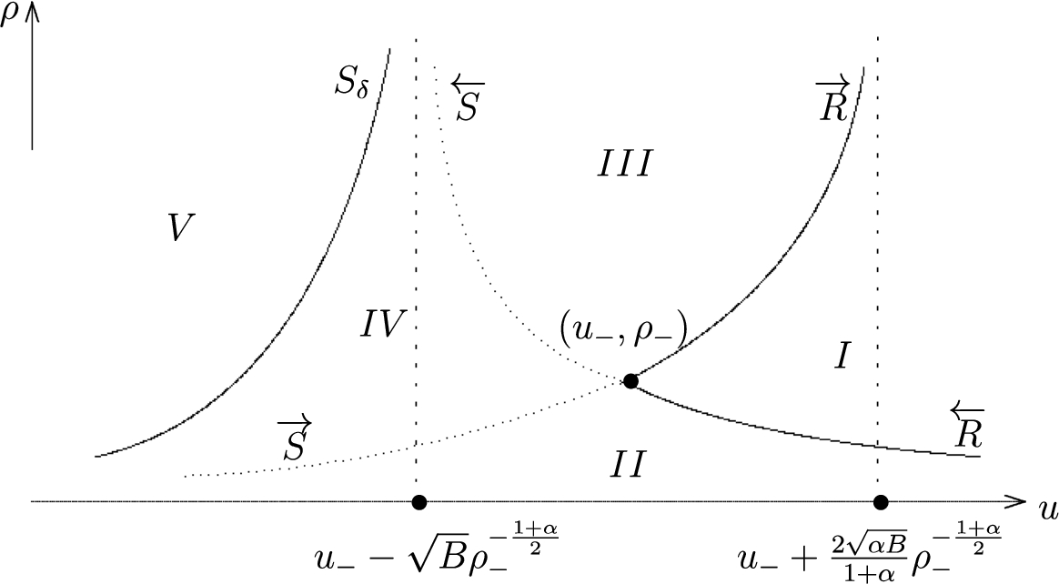
From Lemma 3.2, we know that, when $u_{+} + \sqrt{B} ρ_{+}^{- \frac{1 + α}{2}} ⩽ u_{-} - \sqrt{B} ρ_{-}^{- \frac{1 + α}{2}}$ , we cannot connect the states $(u_{\pm}, ρ_{\pm})$ by two shocks $\overset{\leftarrow}{S} (u_{-}, ρ_{-})$ and $\vec{S} (u_{+}, ρ_{+})$ in $(u, ρ)$ -plane, the phase plane, which tells us that in this situation the solutions must be constructed in the nonclassical sense. Thus, in the $(u, ρ)$ -plane, for any given left state $(u_{-}, ρ_{-})$ , we draw the elementary wave curves passing through this point. The backward shock wave curve $\overset{\leftarrow}{S} (u_{-}, ρ_{-})$ has the asymptotic line $u = u_{-} - \sqrt{B} ρ_{-}^{- \frac{1 + α}{2}}$ , and the forward rarefaction wave curve $\vec{R} (u_{-}, ρ_{-})$ , $u = u_{-} + \frac{2 \sqrt{α B}}{1 + α} ρ_{-}^{- \frac{1 + α}{2}}$ . Besides, motivated by Lemma 3.2, we draw a curve $S_{δ}$ as follows $\begin{array}{l} (3.11) & S_{δ} : u + \sqrt{B} ρ^{- \frac{1 + α}{2}} = u_{-} - \sqrt{B} ρ_{-}^{- \frac{1 + α}{2}}, ρ > 0, \end{array}$ which can be viewed as the boundary of the region where nonclassical solutions appear. Then, the phase plane is divided into five regions I, $II$ , $III$ , $IV$ and $V (u_{-}, ρ_{-})$ , as shown in Fig. 1.

Fig. 1.
Curves of elementary waves of (1.4).

Using these elementary waves: shocks and rarefaction waves, one can construct the solutions of (1.4) and (1.5) by virtue of the analysis method in phase plane. For example, when $(u_{+}, ρ_{+}) \in I (u_{-}, ρ_{-})$ , starting from the point $(u_{+}, ρ_{+})$ , we draw the curve $\vec{R} (u_{+}, ρ_{+})$ , then it must intersect with $\overset{\leftarrow}{R} (u_{-}, ρ_{-})$ at a unique point, so the two constant states $(u_{\pm}, ρ_{\pm})$ can be connected by $\overset{\leftarrow}{R}$ and $\vec{R}$ , as well as an intermediate constant state between them. Therefore, according to the right state $(u_{+}, ρ_{+})$ in the different region, one can construct the unique global Riemann solution connecting two constant states $(u_{\pm}, ρ_{\pm})$ as follows: $\begin{array}{l} (1) (u_{+}, ρ_{+}) \in I (u_{-}, ρ_{-}) : \overset{\leftarrow}{R} + \vec{R}; (2) (u_{+}, ρ_{+}) \in II (u_{-}, ρ_{-}) : \overset{\leftarrow}{R} + \vec{S}; \\ (3) (u_{+}, ρ_{+}) \in III (u_{-}, ρ_{-}) : \overset{\leftarrow}{S} + \vec{R}; (4) (u_{+}, ρ_{+}) \in IV (u_{-}, ρ_{-}) : \overset{\leftarrow}{S} + \vec{S} . \end{array}$

However, when $(u_{+}, ρ_{+}) \in V (u_{-}, ρ_{-})$ , one has $u_{+} < u_{-} - \sqrt{B} ρ_{-}^{- \frac{1 + α}{2}} - \sqrt{B} ρ_{+}^{- \frac{1 + α}{2}}$ , that is, $u_{+} + \sqrt{B} ρ_{+}^{- \frac{1 + α}{2}} < u_{-} - \sqrt{B} ρ_{-}^{- \frac{1 + α}{2}}$ , so we need to seek a nonclassical solution. In fact, from the above discussions, we know that the nonclassical solution may occur under the condition that $u_{+} + \sqrt{B} ρ_{+}^{- \frac{1 + α}{2}} ⩽ u_{-} - \sqrt{B} ρ_{-}^{- \frac{1 + α}{2}}$ . In this situation, we have $\begin{matrix} λ_{1}^{α} (u_{+}, ρ_{+}) < λ_{2}^{α} (u_{+}, ρ_{+}) < λ_{1}^{α} (u_{-}, ρ_{-}) < λ_{2}^{α} (u_{-}, ρ_{-}), \end{matrix}$ namely, $\begin{matrix} u_{+} - \sqrt{α B} ρ_{+}^{- \frac{1 + α}{2}} < u_{+} + \sqrt{α B} ρ_{+}^{- \frac{1 + α}{2}} < u_{-} - \sqrt{α B} ρ_{-}^{- \frac{1 + α}{2}} < u_{-} + \sqrt{α B} ρ_{-}^{- \frac{1 + α}{2}}, \end{matrix}$ which means that the characteristic lines from initial data will overlap in the domain Ω, as shown in Fig. 2. So singularity must happen in Ω. It is well known that the singularity is impossible to be a jump with finite amplitude, which implies that there is no solution that is piecewise smooth and bounded.

Fig. 2.
Analysis of characteristics for delta-shock of (1.4).

Hence, motivated by [26,31,34], etc., the solution for (1.4) with delta distribution at the jump (i.e., the delta-shock solution) should be constructed, which is, under the Definition 2.1, $\begin{array}{l} (3.12) & ρ (t, x) = ρ_{0} (t, x) + \tilde{w} (t) δ_{S}, u (t, x) = u_{0} (t, x), \end{array}$ where $S = {(t, \tilde{σ} t) : 0 ⩽ t < \infty}$ , and $\begin{array}{l} (3.13) & \{\begin{matrix} ρ_{0} (t, x) = ρ_{-} + [ρ] χ (x - \tilde{σ} t), \\ u_{0} (t, x) = u_{-} + [u] χ (x - \tilde{σ} t), \\ \tilde{w} (t) = \frac{t}{\sqrt{1 + {\tilde{σ}}^{2}}} (\tilde{σ} [ρ] - [ρ u]), \end{matrix} \end{array}$ where $\frac{1}{ρ^{α}}$ is defined as $\begin{array}{l} (3.14) & \frac{1}{ρ^{α}} = \{\begin{matrix} \frac{1}{ρ_{-}^{α}}, & x < \tilde{σ} t, \\ 0, & x = \tilde{σ} t, \\ \frac{1}{ρ_{+}^{α}}, & x > \tilde{σ} t . \end{matrix} \end{array}$

By Definition 2.2, one can prove that if (3.12)–(3.14) are the solutions of (1.4), then this kind of discontinuity solution must satisfy the generalized Rankin–Hugoniot relations $\begin{array}{l} (3.15) & \{\begin{matrix} \frac{d x}{d t} = \tilde{σ}, \\ \frac{d (\tilde{w} (t) \sqrt{1 + {\tilde{σ}}^{2}})}{d t} = \tilde{σ} [ρ] - [ρ u], \\ \frac{d (\tilde{w} (t) \tilde{σ} \sqrt{1 + {\tilde{σ}}^{2}})}{d t} = \tilde{σ} [ρ u] - [ρ u^{2} - \frac{B}{ρ^{α}}] . \end{matrix} \end{array}$ In addition, to guarantee the uniqueness, the discontinuity must obey the entropy condition $\begin{array}{l} (3.16) & u_{+} + \sqrt{α B} ρ_{+}^{- \frac{1 + α}{2}} < \tilde{σ} < u_{-} - \sqrt{α B} ρ_{-}^{- \frac{1 + α}{2}}, \end{array}$ which ensures that all the characteristic lines on both sides of the discontinuity are in-coming. A discontinuity satisfying (3.15) and (3.16) is called a delta shock wave to the system (1.4).

By solving the generalized Rankine–Hugoniot relation (3.15) with initial data $x (0) = 0$ and $\tilde{w} (0) = 0$ , we have $\begin{array}{l} (3.17) & \tilde{σ} = \frac{[ρ u] + \sqrt{ρ_{-} ρ_{+} {[u]}^{2} - [ρ] [- \frac{B}{ρ^{α}}]}}{[ρ]}, \tilde{w} (t) = \frac{\sqrt{ρ_{-} ρ_{+} {[u]}^{2} - [ρ] [- \frac{B}{ρ^{α}}]}}{\sqrt{1 + {\tilde{σ}}^{2}}} t \end{array}$ as $ρ_{-} \neq ρ_{+}$ , and $\begin{array}{l} (3.18) & \tilde{σ} = \frac{u_{-} + u_{+}}{2}, \tilde{w} (t) = \frac{ρ_{-} u_{-} - ρ_{+} u_{+}}{\sqrt{1 + {\tilde{σ}}^{2}}} t \end{array}$ as $ρ_{-} = ρ_{+}$ .

Thus, when $(u_{+}, ρ_{+}) \in V (u_{-}, ρ_{-})$ , the solution of (1.4) consists of a delta shock wave. That is, the two states $(u_{-}, ρ_{-})$ and $(u_{+}, ρ_{+})$ can be directly connected by a delta shock wave.

So far, we have completed the construction of the Riemann solutions to the system (1.4).
Remark 3.1.
When $α = 1$ , the system (1.4) corresponds to Chaplygin gas equations. One can check from (3.1) and (3.2) that $\nabla λ_{i}^{α} \cdot {\vec{r}}_{i}^{α} \equiv 0$ ( $i = 1, 2$ ), which implies that both the characteristic fields are linearly degenerate and the elementary waves involve only contact discontinuities. That is to say, at this time, both the backward (forward) rarefaction wave and the backward (forward) shock wave become the backward (forward) contact discontinuity.
4. Riemann problem to the extended Chaplygin gas equations

We now solve the Riemann problem (1.1) and (1.5).

The system (1.1) has two eigenvalues $\begin{array}{l} (4.1) & λ_{1}^{α γ} = u - \sqrt{\frac{A γ}{ρ^{1 - γ}} + \frac{α B}{ρ^{α + 1}}}, λ_{2}^{α γ} = u + \sqrt{\frac{A γ}{ρ^{1 - γ}} + \frac{α B}{ρ^{α + 1}}}, \end{array}$ with two associated right eigenvectors $\begin{array}{l} (4.2) & {\vec{r_{1}}}^{α γ} = {(\sqrt{\frac{A γ}{ρ^{1 - γ}} + \frac{α B}{ρ^{α + 1}}}, - ρ)}^{T}, {\vec{r_{2}}}^{α γ} = {(\sqrt{\frac{A γ}{ρ^{1 - γ}} + \frac{α B}{ρ^{α + 1}}}, ρ)}^{T} . \end{array}$ Since one can check that $\begin{matrix} \nabla λ_{i}^{α γ} \cdot {\vec{r_{i}}}^{α γ} = \frac{A γ (γ + 1) ρ^{α + γ} + α (1 - α) B}{2 \sqrt{(A γ ρ^{α + γ} + α B) ρ^{α + 1}}} > 0, (i = 1, 2) \end{matrix}$ for $α, γ \in (0, 1)$ , so (1.4) is strictly hyperbolic and the characteristics are genuinely nonlinear.

By a self-similar transformation $ξ = x / t$ , the Riemann problem (1.4) and (1.5) is reduced to a boundary value problem $\begin{array}{l} (4.3) & \{\begin{matrix} - ξ ρ_{ξ} + {(ρ u)}_{ξ} = 0, \\ - ξ {(ρ u)}_{ξ} + {(ρ u^{2} + A ρ^{γ} - \frac{B}{ρ^{α}})}_{ξ} = 0, \\ (u, ρ) (\pm \infty) = (u_{\pm}, ρ_{\pm}), \end{matrix} \end{array}$ which provides either the constant solution or the backward rarefaction wave $\begin{array}{l} (4.4) & R_{1} (u_{-}, ρ_{-}) : \{\begin{matrix} ξ = λ_{1}^{α γ} = u - \sqrt{\frac{A γ}{ρ^{1 - γ}} + \frac{α B}{ρ^{α + 1}}}, \\ d u + \frac{\sqrt{\frac{A γ}{ρ^{1 - γ}} + \frac{α B}{ρ^{α + 1}}}}{ρ} d ρ = 0 \end{matrix} \end{array}$ or the forward rarefaction wave $\begin{array}{l} (4.5) & R_{2} (u_{-}, ρ_{-}) : \{\begin{matrix} ξ = λ_{2}^{α γ} = u + \sqrt{\frac{A γ}{ρ^{1 - γ}} + \frac{α B}{ρ^{α + 1}}}, \\ d u - \frac{\sqrt{\frac{A γ}{ρ^{1 - γ}} + \frac{α B}{ρ^{α + 1}}}}{ρ} d ρ = 0 . \end{matrix} \end{array}$

We can deduce from (4.4) and (4.5) that $\begin{array}{l} \frac{d λ_{1}^{α γ}}{d ρ} & = \frac{\partial λ_{1}^{α γ}}{\partial u} \cdot \frac{d u}{d ρ} + \frac{\partial λ_{1}^{α γ}}{\partial ρ} = - \frac{\sqrt{\frac{A γ}{ρ^{1 - γ}} + \frac{α B}{ρ^{α + 1}}}}{ρ} - \frac{A γ (γ - 1) ρ^{γ - 2} - \frac{α (α + 1) B}{ρ^{α + 2}}}{2 \sqrt{\frac{A γ}{ρ^{1 - γ}} + \frac{α B}{ρ^{α + 1}}}} \\ (4.6) & = - \frac{A γ (γ + 1) ρ^{γ - 1} + \frac{α (1 - α) B}{ρ^{α + 1}}}{2 ρ \sqrt{\frac{A γ}{ρ^{1 - γ}} + \frac{α B}{ρ^{α + 1}}}} < 0 . \end{array}$ Similarly, for $λ_{2}^{α γ}$ , we have $\begin{array}{l} (4.7) & \frac{d λ_{2}^{α γ}}{d ρ} = \frac{\partial λ_{2}^{α γ}}{\partial u} \cdot \frac{d u}{d ρ} + \frac{\partial λ_{2}^{α γ}}{\partial ρ} = \frac{A γ (γ + 1) ρ^{γ - 1} + \frac{α (1 - α) B}{ρ^{α + 1}}}{2 ρ \sqrt{\frac{A γ}{ρ^{1 - γ}} + \frac{α B}{ρ^{α + 1}}}} > 0 . \end{array}$ The equalities (4.6) and (4.7) show that the velocity of backward (forward) rarefaction wave $λ_{1}^{α γ}$ ( $λ_{2}^{α γ}$ ) is monotonically decreasing (increasing) with respect to ρ.

Considering that $λ_{1}^{α γ} (u, ρ) > λ_{1}^{α γ} (u_{-}, ρ_{-})$ and $λ_{2}^{α γ} (u, ρ) > λ_{2}^{α γ} (u_{-}, ρ_{-})$ , we have, by integrating the second equations of (4.4) and (4.5) respectively, $\begin{array}{l} (4.8) & R_{1} (u_{-}, ρ_{-}) : \{\begin{matrix} ξ = λ_{1}^{α γ} = u - \sqrt{\frac{A γ}{ρ^{1 - γ}} + \frac{α B}{ρ^{α + 1}}}, \\ u = u_{-} - \int_{ρ_{-}}^{ρ} \frac{\sqrt{\frac{A γ}{s^{1 - γ}} + \frac{α B}{s^{α + 1}}}}{s} d s, ρ < ρ_{-} \end{matrix} \end{array}$ and $\begin{array}{l} (4.9) & R_{2} (u_{-}, ρ_{-}) : \{\begin{matrix} ξ = λ_{2}^{α γ} = u + \sqrt{\frac{A γ}{ρ^{1 - γ}} + \frac{α B}{ρ^{α + 1}}}, \\ u = u_{-} + \int_{ρ_{-}}^{ρ} \frac{\sqrt{\frac{A γ}{s^{1 - γ}} + \frac{α B}{s^{α + 1}}}}{s} d s, ρ > ρ_{-} . \end{matrix} \end{array}$

The rarefaction wave curves enjoy the following geometric properties.

Lemma 4.1.
For the rarefaction wave curves $R_{1}$ and $R_{2}$ based on $(u_{-}, ρ_{-})$ , we have $\begin{matrix} R_{1} (u_{-}, ρ_{-}) : \frac{d u}{d ρ} < 0, lim_{ρ \to 0^{+}} u = + \infty; R_{2} (u_{-}, ρ_{-}) : \frac{d u}{d ρ} > 0, lim_{ρ \to + \infty} u = l_{a} < + \infty, \end{matrix}$ where $l_{a}$ is a constant.
Proof.
For the back rarefaction wave curve $R_{1} (u_{-}, ρ_{-})$ , it follows from the second equation of (4.8) that $\begin{matrix} R_{1} (u_{-}, ρ_{-}) : \frac{d u}{d ρ} = - \frac{\sqrt{\frac{A γ}{ρ^{1 - γ}} + \frac{α B}{ρ^{α + 1}}}}{ρ} < 0 . \end{matrix}$ Similarly, one has $\frac{d u}{d ρ} > 0$ on $R_{2} (u_{-}, ρ_{-})$ .

Now, let us investigate the geometric properties of rarefaction wave curves. We will consider $R_{1} (u_{-}, ρ_{-})$ curve first. In this situation, $\begin{array}{l} (4.10) & u = u_{-} - I (ρ), ρ < ρ_{-}, \end{array}$ where $\begin{array}{l} (4.11) & I (ρ) = \int_{ρ_{-}}^{ρ} f (s) d s and f (ρ) = \frac{\sqrt{\frac{A γ}{ρ^{1 - γ}} + \frac{α B}{ρ^{α + 1}}}}{ρ} . \end{array}$

Denoted by $\begin{array}{l} (4.12) & I_{0} (ρ) = \int_{ρ_{-}}^{ρ} f_{0} (s) d s and f_{0} (ρ) = \frac{\sqrt{\frac{A γ}{ρ^{1 - γ}}}}{ρ}, \end{array}$ then one can calculate that $\begin{matrix} I_{0} (ρ) = \sqrt{A γ} \int_{ρ_{-}}^{ρ} s^{\frac{γ - 1}{2} - 1} d s = \frac{2 \sqrt{A γ}}{1 - γ} (ρ_{-}^{\frac{γ - 1}{2}} - ρ^{\frac{γ - 1}{2}}), \end{matrix}$ which implies that ${lim}_{ρ \to 0^{+}} I_{0} (ρ) = - \infty$ . Noting that $\begin{matrix} lim_{ρ \to 0^{+}} \frac{f (ρ)}{f_{0} (ρ)} = lim_{ρ \to 0^{+}} \frac{\sqrt{\frac{A γ}{ρ^{1 - γ}} + \frac{α B}{ρ^{α + 1}}}}{\sqrt{\frac{A γ}{ρ^{1 - γ}}}} = lim_{ρ \to 0^{+}} \sqrt{1 + \frac{α B}{A γ} \cdot \frac{1}{ρ^{α + γ}}} = + \infty, \end{matrix}$ so ${lim}_{ρ \to 0^{+}} I (ρ) = - \infty$ . Owing to (4.10), we know that ${lim}_{ρ \to 0^{+}} u = + \infty$ on $R_{1} (u_{-}, ρ_{-})$ .

Let us turn to $R_{2} (u_{-}, ρ_{-})$ . Along this curve, one has $\begin{array}{l} (4.13) & u = u_{-} + I (ρ), ρ > ρ_{-}, \end{array}$ where $I (ρ)$ is defined in (4.11). Since ${lim}_{ρ \to + \infty} \frac{f (ρ)}{f_{0} (ρ)} = 1$ and ${lim}_{ρ \to + \infty} I_{0} (ρ) = \frac{2 \sqrt{A γ}}{1 - γ} ρ_{-}^{\frac{γ - 1}{2}}$ , thus ${lim}_{ρ \to + \infty} I (ρ)$ exists, which means that ${lim}_{ρ \to + \infty} u = l_{a}$ along $R_{2} (u_{-}, ρ_{-})$ . This finishes the proof of Lemma 4.1. □

For the bounded discontinuity at $ξ = ω$ , it satisfies the Rankine–Hugoniot condition $\begin{array}{l} (4.14) & \{\begin{matrix} ω [ρ] = [ρ u], \\ ω [ρ u] = [ρ u^{2} + A ρ^{γ} - \frac{B}{ρ^{α}}], \end{matrix} \end{array}$ where ω is the velocity of the shock.

Eliminating ω in (4.14) gives $\begin{array}{l} (4.15) & {(u - u_{-})}^{2} = \frac{ρ_{-} - ρ}{ρ_{-} ρ} (A (ρ_{-}^{γ} - ρ^{γ}) + B (\frac{1}{ρ^{α}} - \frac{1}{ρ_{-}^{α}})) . \end{array}$ Then, one has $\begin{array}{l} (4.16) & u - u_{-} = \pm \sqrt{(\frac{1}{ρ_{-}} - \frac{1}{ρ}) (A (ρ^{γ} - ρ_{-}^{γ}) + B (\frac{1}{ρ_{-}^{α}} - \frac{1}{ρ^{α}}))} . \end{array}$

Moreover, in order to identify the admissible solution, the shock wave should satisfy the stability condition $\begin{array}{l} (4.17) & ω < λ_{1}^{α γ} (u_{-}, ρ_{-}) < λ_{2}^{α γ} (u_{-}, ρ_{-}), λ_{1}^{α γ} (u, ρ) < ω < λ_{2}^{α γ} (u, ρ), \end{array}$ for $S_{1}$ associating with $λ_{1}^{α γ}$ ; and $\begin{array}{l} (4.18) & λ_{1}^{α γ} (u_{-}, ρ_{-}) < ω < λ_{2}^{α γ} (u_{-}, ρ_{-}), λ_{1}^{α γ} (u, ρ) < λ_{2}^{α γ} (u, ρ) < ω, \end{array}$ for $S_{2}$ associating with $λ_{2}^{α γ}$ .

It yields from the first equation of (4.14) that $\begin{array}{l} (4.19) & ω = \frac{ρ u - ρ_{-} u_{-}}{ρ - ρ_{-}} = u + \frac{ρ_{-} (u - u_{-})}{ρ - ρ_{-}} = u_{-} + \frac{ρ (u - u_{-})}{ρ - ρ_{-}} . \end{array}$ Together with (4.17) and (4.19), we have $\begin{array}{l} (4.20) & - ρ \sqrt{\frac{A γ}{ρ^{1 - γ}} + \frac{α B}{ρ^{α + 1}}} < \frac{ρ ρ_{-} (u - u_{-})}{ρ - ρ_{-}} < - ρ_{-} \sqrt{\frac{A γ}{ρ_{-}^{1 - γ}} + \frac{α B}{ρ_{-}^{α + 1}}}, \end{array}$ which means that $ρ > ρ_{-}$ and $u < u_{-}$ for $S_{1}$ .

Similarly, (4.18) and (4.19) yield that $\begin{array}{l} (4.21) & ρ \sqrt{\frac{A γ}{ρ^{1 - γ}} + \frac{α B}{ρ^{α + 1}}} < \frac{ρ ρ_{-} (u - u_{-})}{ρ - ρ_{-}} < ρ_{-} \sqrt{\frac{A γ}{ρ_{-}^{1 - γ}} + \frac{α B}{ρ_{-}^{α + 1}}}, \end{array}$ which implies that $ρ < ρ_{-}$ and $u < u_{-}$ for $S_{2}$ .

Thereby, associating with $λ_{1}^{α γ}$ , we obtain the backward shock wave $\begin{array}{l} (4.22) & S_{1} (u_{-}, ρ_{-}) : \{\begin{matrix} ω_{1} = u_{-} - ρ \sqrt{\frac{1}{ρ_{-} ρ (ρ - ρ_{-})} \cdot (A (ρ^{γ} - ρ_{-}^{γ}) + B (\frac{1}{ρ_{-}^{α}} - \frac{1}{ρ^{α}}))}, \\ u = u_{-} - \sqrt{(\frac{1}{ρ_{-}} - \frac{1}{ρ}) \cdot (A (ρ^{γ} - ρ_{-}^{γ}) + B (\frac{1}{ρ_{-}^{α}} - \frac{1}{ρ^{α}}))}, ρ > ρ_{-}, \end{matrix} \end{array}$ and associating with $λ_{2}^{α γ}$ , we get the forward shock wave $\begin{array}{l} (4.23) & S_{2} (u_{-}, ρ_{-}) : \{\begin{matrix} ω_{2} = u_{-} + ρ \sqrt{\frac{1}{ρ_{-} ρ (ρ - ρ_{-})} \cdot (A (ρ^{γ} - ρ_{-}^{γ}) + B (\frac{1}{ρ_{-}^{α}} - \frac{1}{ρ^{α}}))}, \\ u = u_{-} - \sqrt{(\frac{1}{ρ_{-}} - \frac{1}{ρ}) \cdot (A (ρ^{γ} - ρ_{-}^{γ}) + B (\frac{1}{ρ_{-}^{α}} - \frac{1}{ρ^{α}}))}, ρ < ρ_{-} . \end{matrix} \end{array}$

Moreover, we have the following result
Lemma 4.2.
For the shock wave curves based on the left state $(u_{-}, ρ_{-})$ , we have $\begin{array}{l} (4.24) & S_{1} (u_{-}, ρ_{-}) : \frac{d u}{d ρ} < 0, lim_{ρ \to + \infty} u = - \infty; S_{2} (u_{-}, ρ_{-}) : \frac{d u}{d ρ} > 0, lim_{ρ \to 0^{+}} u = - \infty . \end{array}$
Proof.
Differentiating u with respect to ρ in (4.15) gives that $\begin{array}{l} (4.25) & 2 (u - u_{-}) \frac{d u}{d ρ} = \frac{1}{ρ^{2}} (A (ρ^{γ} - ρ_{-}^{γ}) + B (\frac{1}{ρ_{-}^{α}} - \frac{1}{ρ^{α}})) + \frac{ρ - ρ_{-}}{ρ ρ_{-}} (\frac{A γ}{ρ^{1 - γ}} + \frac{α B}{ρ^{α + 1}}) . \end{array}$ Noting that $u - u_{-} < 0$ , the above equality shows that $\frac{d u}{d ρ} < 0$ on $S_{1}$ since $ρ > ρ_{-}$ , and $\frac{d u}{d ρ} > 0$ on $S_{2}$ since $ρ < ρ_{-}$ . Furthermore, from the second equations of (4.22) and (4.23), one can easily observe that ${lim}_{ρ \to + \infty} u = - \infty$ on $S_{1}$ , and ${lim}_{ρ \to 0^{+}} u = - \infty$ on $S_{2}$ . The proof is completed. □

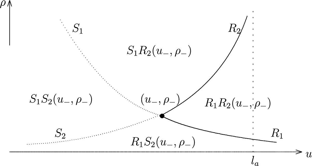
According to the geometric properties of the curves for rarefaction wave and shock wave, we know that, for the given left state $(u_{-}, ρ_{-})$ , the half-upper $(u, ρ)$ -phase plane is divided into four regions by the curves $R_{1} (u_{-}, ρ_{-})$ , $S_{1} (u_{-}, ρ_{-})$ , $R_{2} (u_{-}, ρ_{-})$ and $S_{2} (u_{-}, ρ_{-})$ starting from the point $(u_{-}, ρ_{-})$ , as shown in Fig. 3. These four regions, denoted by $R_{1} R_{2} (u_{-}, ρ_{-})$ , $R_{1} S_{2} (u_{-}, ρ_{-})$ , $S_{1} R_{2} (u_{-}, ρ_{-})$ and $S_{1} S_{2} (u_{-}, ρ_{-})$ , respectively, correspond to four kinds of configurations of Riemann solutions to the extended Chaplygin gas equations (1.1), which can be represented by the symbols $R_{1} + R_{2}$ , $R_{1} + S_{2}$ , $S_{1} + R_{2}$ or $S_{1} + S_{2}$ , respectively, where the symbol “+” means “followed by”.

Fig. 3.
Curves of elementary waves of (1.1).
5. Formation of delta shock waves and vacuums as $α, γ \to 0$

In this section, we study the limits of Riemann solutions to the extended Chaplygin gas equations (1.1) with the initial data (1.5) as both the two exponents $α, γ \to 0$ , that is, the extended Chaplygin gas pressure $p (ρ) = A ρ^{γ} - \frac{B}{ρ^{α}}$ tends to a constant $A - B$ . We will first discuss the formation of delta shock waves in the Riemann solutions of (1.1) and (1.5) in the case $(u_{+}, ρ_{+}) \in S_{1} S_{2} (u_{-}, ρ_{-})$ with $u_{-} > u_{+}$ , then analyze the formation of vacuum states in the case $(u_{+}, ρ_{+}) \in R_{1} R_{2} (u_{-}, ρ_{-})$ with $u_{-} < u_{+}$ and $ρ_{\pm} > 0$ , as $α, γ \to 0$ .

5.1. Limit behavior of Riemann solutions as $α, γ \to 0$

For each pair of fixed α and γ, if $(u_{-}, ρ_{-})$ and $(u_{*}, ρ_{*})$ are connected by a $S_{1}$ with speed $ω_{1}$ , and that $(u_{*}, ρ_{*})$ and $(u_{+}, ρ_{+})$ are connected by a $S_{2}$ with speed $ω_{2}$ , then it follows that $\begin{array}{l} (5.1) & S_{1} : \{\begin{matrix} ω_{1} = u_{-} - ρ_{*} \sqrt{\frac{1}{ρ_{-} ρ_{*} (ρ_{*} - ρ_{-})} \cdot (A (ρ_{*}^{γ} - ρ_{-}^{γ}) + B (\frac{1}{ρ_{-}^{α}} - \frac{1}{ρ_{*}^{α}}))}, \\ u_{*} = u_{-} - \sqrt{(\frac{1}{ρ_{-}} - \frac{1}{ρ_{*}}) \cdot (A (ρ_{*}^{γ} - ρ_{-}^{γ}) + B (\frac{1}{ρ_{-}^{α}} - \frac{1}{ρ_{*}^{α}}))}, ρ_{*} > ρ_{-}, \end{matrix} \end{array}$ and $\begin{array}{l} (5.2) & S_{2} : \{\begin{matrix} ω_{2} = u_{*} + ρ_{+} \sqrt{\frac{1}{ρ_{*} ρ_{+} (ρ_{+} - ρ_{*})} \cdot (A (ρ_{+}^{γ} - ρ_{*}^{γ}) + B (\frac{1}{ρ_{*}^{α}} - \frac{1}{ρ_{+}^{α}}))}, \\ u_{+} = u_{*} - \sqrt{(\frac{1}{ρ_{*}} - \frac{1}{ρ_{+}}) \cdot (A (ρ_{+}^{γ} - ρ_{*}^{γ}) + B (\frac{1}{ρ_{*}^{α}} - \frac{1}{ρ_{+}^{α}}))}, ρ_{*} > ρ_{+} . \end{matrix} \end{array}$ We have, together with (5.1) and (5.2), $\begin{array}{l} u_{-} - u_{+} = & \sqrt{(\frac{1}{ρ_{-}} - \frac{1}{ρ_{*}}) \cdot (A (ρ_{*}^{γ} - ρ_{-}^{γ}) + B (\frac{1}{ρ_{-}^{α}} - \frac{1}{ρ_{*}^{α}}))} \\ (5.3) & + \sqrt{(\frac{1}{ρ_{*}} - \frac{1}{ρ_{+}}) \cdot (A (ρ_{+}^{γ} - ρ_{*}^{γ}) + B (\frac{1}{ρ_{*}^{α}} - \frac{1}{ρ_{+}^{α}}))} . \end{array}$

In order to discuss the limit behavior of Riemann solutions of (1.1) and (1.5) as $α, γ \to 0$ , we should prove some useful lemmas.

Lemma 5.1.
It holds that $\begin{matrix} lim_{α, γ \to 0} ρ_{} = + \infty \end{matrix}$ and* $\begin{matrix} lim_{α, γ \to 0} (A ρ_{}^{γ} - \frac{B}{ρ_{}^{α}}) : = θ = A - B + {(\frac{(u_{-} - u_{+}) \sqrt{ρ_{-} ρ_{+}}}{\sqrt{ρ_{-}} + \sqrt{ρ_{+}}})}^{2} . \end{matrix}$
Proof.
Set ${lim}_{α, γ \to 0} inf ρ_{} = a$ , ${lim}_{α, γ \to 0} sup ρ_{} = b$ . This lemma will be proved by the following three steps.

(i). At first, we show that $a = b$ . Here, just for convenience of the prove, we suppose that $α = γ$ . If $a < b$ , then by the continuity of $ρ_{} (α)$ , there exists a sequence ${α_{n}}_{n = 1}^{\infty} \subset (0, 1)$ such that $\begin{matrix} lim_{n \to \infty} α_{n} = 0 and lim_{n \to \infty} ρ_{} (α_{n}) = c \end{matrix}$ for some $c \in (a, b)$ . Then, substituting the sequence into the right of (5.3) and taking the limit yields that $\begin{array}{l} u_{-} - u_{+} = & lim_{n \to \infty} \sqrt{(\frac{1}{ρ_{-}} - \frac{1}{ρ_{} (α_{n})}) \cdot (A (ρ_{} {(α_{n})}^{α_{n}} - ρ_{-}^{α_{n}}) + B (\frac{1}{ρ_{-}^{α_{n}}} - \frac{1}{ρ_{} {(α_{n})}^{α_{n}}}))} \\ + lim_{n \to \infty} \sqrt{(\frac{1}{ρ_{} (α_{n})} - \frac{1}{ρ_{+}}) \cdot (A (ρ_{+}^{α_{n}} - ρ_{} {(α_{n})}^{α_{n}}) + B (\frac{1}{ρ_{} {(α_{n})}^{α_{n}}} - \frac{1}{ρ_{+}^{α_{n}}}))} \\ = & 0, \end{array}$ which contradicts with the fact that $u_{-} > u_{+}$ . Hence, we have $a = b$ .

(ii). We show that ${lim}_{α, γ \to 0} ρ_{} = + \infty$ . If $a = b \in (0, + \infty)$ , then denoted by ${lim}_{α, γ \to 0} ρ_{} = a$ . By a similar method used above, one can also obtain a contradiction when taking limit in (5.3). Therefore, $a = b = 0$ or $a = b = + \infty$ . However, from the entropy condition we know that $ρ_{} > max {ρ_{-}, ρ_{+}}$ , which yields that ${lim}_{α, γ \to 0} ρ_{} (α, γ) = + \infty$ .

(iii). Noticing that $\begin{array}{l} lim_{α, γ \to 0} (\frac{1}{ρ_{\pm}} - \frac{1}{ρ_{}}) \cdot (A (ρ_{}^{γ} - ρ_{\pm}^{γ}) + B (\frac{1}{ρ_{\pm}^{α}} - \frac{1}{ρ_{}^{α}})) \\ = lim_{α, γ \to 0} \frac{ρ_{} - ρ_{\pm}}{ρ_{\pm} ρ_{}} \cdot ((A ρ_{}^{γ} - \frac{B}{ρ_{}^{α}}) - (A ρ_{\pm}^{γ} - \frac{1}{ρ_{\pm}^{α}})) \\ = \frac{θ - (A - B)}{ρ_{\pm}} . \end{array}$ Thus, letting $α, γ \to 0$ in (5.3), one has $\begin{array}{l} u_{-} - u_{+} = \sqrt{\frac{θ - (A - B)}{ρ_{-}}} + \sqrt{\frac{θ - (A - B)}{ρ_{+}}}, \end{array}$ from which we can solve that $θ = A - B + {(\frac{(u_{-} - u_{+}) \sqrt{ρ_{-} ρ_{+}}}{\sqrt{ρ_{-}} + \sqrt{ρ_{+}}})}^{2}$ . The proof is finished. □
Lemma 5.2.
${lim}_{α, γ \to 0} u_{} = {lim}_{α, γ \to 0} ω_{1} = {lim}_{α, γ \to 0} ω_{2} = σ = \frac{\sqrt{ρ_{-}} u_{-} + \sqrt{ρ_{+}} u_{+}}{\sqrt{ρ_{-}} + \sqrt{ρ_{+}}}$ .
Proof.
By a direct computation, we have $\begin{array}{l} lim_{α, γ \to 0} u_{} = & u_{-} - lim_{α, γ \to 0} \sqrt{(\frac{1}{ρ_{-}} - \frac{1}{ρ_{}}) \cdot (A (ρ_{}^{γ} - ρ_{-}^{γ}) + B (\frac{1}{ρ_{-}^{α}} - \frac{1}{ρ_{}^{α}}))} \\ = & u_{-} - \sqrt{\frac{θ - (A - B)}{ρ_{-}}} \\ = & \frac{\sqrt{ρ_{-}} u_{-} + \sqrt{ρ_{+}} u_{+}}{\sqrt{ρ_{-}} + \sqrt{ρ_{+}}} = σ . \end{array}$

Form the generalized Rankine–Hugoniot condition (4.14), we can derive that $\begin{matrix} lim_{α, γ \to 0} ω_{1} = lim_{α, γ \to 0} \frac{ρ_{} u_{} - ρ_{-} u_{-}}{ρ_{} - ρ_{-}} = lim_{α, γ \to 0} \frac{u_{} - ρ_{-} u_{-} / ρ_{}}{1 - ρ_{-} / ρ_{}} = lim_{α, γ \to 0} u_{} = σ, \end{matrix}$ and $\begin{matrix} lim_{α, γ \to 0} ω_{2} = lim_{α, γ \to 0} \frac{ρ_{+} u_{+} - ρ_{} u_{}}{ρ_{+} - ρ_{}} = lim_{α, γ \to 0} \frac{ρ_{+} u_{+} / ρ_{} - u_{}}{ρ_{+} / ρ_{} - 1} = lim_{α, γ \to 0} u_{} = σ . \end{matrix}$ Thus, Lemma 5.2 is right. □
Lemma 5.3.
$\begin{matrix} lim_{α, γ \to 0} ρ_{} (ω_{2} - ω_{1}) = σ [ρ] - [ρ u], \end{matrix}$

and* $\begin{matrix} lim_{α, γ \to 0} ρ_{} u_{} (ω_{2} - ω_{1}) = σ [ρ u] - [ρ u^{2}] . \end{matrix}$
Proof.
The first equations of the Rankine–Hugoniot relation (4.14) for $S_{1}$ and $S_{2}$ read $\begin{array}{l} \{\begin{matrix} ω_{1} (ρ_{} - ρ_{-}) = ρ_{} u_{} - ρ_{-} u_{-}, \\ ω_{2} (ρ_{+} - ρ_{}) = ρ_{+} u_{+} - ρ_{} u_{}, \end{matrix} \end{array}$ from which one has $\begin{array}{l} lim_{α, γ \to 0} ρ_{} (ω_{2} - ω_{1}) = lim_{α, γ \to 0} (ρ_{+} ω_{2} - ρ_{+} u_{+} - ρ_{-} ω_{1} + ρ_{-} u_{-}) = σ [ρ] - [ρ u] . \end{array}$

Similarly, we obtain from the second equations of the Rankine–Hugoniot relation (4.14) for $S_{1}$ and $S_{2}$ that $\begin{array}{l} \{\begin{matrix} ω_{1} (ρ_{} u_{} - ρ_{-} u_{-}) = ρ_{} u_{}^{2} - ρ_{-} u_{-}^{2} + (A ρ_{}^{γ} - \frac{B}{ρ_{}^{α}}) - (A ρ_{-}^{γ} - \frac{B}{ρ_{-}^{α}}), \\ ω_{2} (ρ_{+} u_{+} - ρ_{} u_{}) = ρ_{+} u_{+}^{2} - ρ_{} u_{}^{2} + (A ρ_{+}^{γ} - \frac{B}{ρ_{+}^{α}}) - (A ρ_{}^{γ} - \frac{B}{ρ_{}^{α}}), \end{matrix} \end{array}$ which yields that $\begin{array}{l} lim_{α, γ \to 0} ρ_{} u_{} (ω_{2} - ω_{1}) \\ = lim_{α, γ \to 0} (ρ_{+} u_{+} ω_{2} - ρ_{+} u_{+}^{2} - (A ρ_{+}^{γ} - \frac{B}{ρ_{+}^{α}}) - ρ_{-} u_{-} ω_{1} + ρ_{-} u_{-}^{2} + (A ρ_{-}^{γ} - \frac{B}{ρ_{-}^{α}})) \\ = σ [ρ u] - [ρ u^{2}] . \end{array}$ This is the end of the proof. □
Remark 5.1.
The above lemmas imply that, as the exponents α and γ tend to zero, the two shock waves $S_{1}$ and $S_{2}$ will coincide, and the intermediate density $ρ_{}$ becomes singular. Moreover, the velocities $ω_{1}$ , $ω_{2}$ and $u_{*}$ approach the quantity σ, which uniquely determines the delta-shock solution of (1.3) as the limit of the Riemann solutions to (1.1) and (1.5).

5.2. Formation of delta shock waves as $α, γ \to 0$

Now, as the exponents α and γ vanish, we give the following theorem to well characterize the limits of solutions of (1.1) in the case $(u_{+}, ρ_{+}) \in S_{1} S_{2} (u_{-}, ρ_{-})$ .

Theorem 5.1.
Let $u_{-} > u_{+}$ . For each pair of fixed $α, γ \in (0, 1)$ , assume that $(u_{α γ}, ρ_{α γ})$ is a solution containing two shocks $S_{1}$ and $S_{2}$ of ( 1.1 ), ( 1.5 ) constructed in Section 4 . Then, $ρ_{α γ}$ and $ρ_{α γ} u_{α γ}$ converge in the sense of distributions as $α, γ \to 0$ , and the limit functions ρ and $ρ u$ are the sums of a step function and a Dirac delta function with weights $\begin{array}{l} \frac{t}{\sqrt{1 + σ^{2}}} (σ [ρ] - [ρ u]) and \frac{t}{\sqrt{1 + σ^{2}}} (σ [ρ u] - [ρ u^{2}]), \end{array}$ respectively, which form the delta-shock solution of ( 1.3 ), ( 1.5 ).
Proof.
(i). Set $ξ = x / t$ . For any fixed $α, γ \in (0, 1)$ , the two-shock Riemann solution of (1.1) reads $\begin{array}{l} (u_{α γ}, ρ_{α γ}) (ξ) = \{\begin{matrix} (u_{-}, ρ_{-}), & ξ < ω_{1}, \\ (u_{}, ρ_{}), & ω_{1} < ξ < ω_{2}, \\ (u_{+}, ρ_{+}), & ξ > ω_{2}, \end{matrix} \end{array}$ which satisfies $\begin{array}{l} (5.4) & - \int_{- \infty}^{+ \infty} ρ_{α γ} (u_{α γ} - ξ) ϕ^{'} d ξ + \int_{- \infty}^{+ \infty} ρ_{α γ} ϕ d ξ = 0 \end{array}$ and $\begin{array}{l} (5.5) & \begin{matrix} - \int_{- \infty}^{+ \infty} ρ_{α γ} u_{α γ} (u_{α γ} - ξ) ϕ^{'} d ξ - \int_{- \infty}^{+ \infty} (A {(ρ_{α γ})}^{γ} - \frac{B}{{(ρ_{α γ})}^{α}}) ϕ^{'} d ξ \\ + \int_{- \infty}^{+ \infty} ρ_{α γ} u_{α γ} ϕ d ξ = 0 \end{matrix} \end{array}$ for any $ϕ \in C_{0}^{\infty} (- \infty, + \infty)$ .

(ii). Let us discuss the limits of $ρ_{α γ} u_{α γ}$ and $ρ_{α γ}$ depending on ξ. The first integral on the left of (5.5) can be decomposed as $\begin{array}{l} (5.6) & \int_{- \infty}^{+ \infty} ρ_{α γ} u_{α γ} (u_{α γ} - ξ) ϕ^{'} d ξ = (\int_{- \infty}^{ω_{1}} + \int_{ω_{1}}^{ω_{2}} + \int_{ω_{2}}^{+ \infty}) ρ_{α γ} u_{α γ} (u_{α γ} - ξ) ϕ^{'} d ξ . \end{array}$ For the first and last terms of (5.6), it can be calculated that $\begin{array}{l} lim_{α, γ \to 0} (\int_{- \infty}^{ω_{1}} + \int_{ω_{2}}^{+ \infty}) ρ_{α γ} u_{α γ} (u_{α γ} - ξ) ϕ^{'} d ξ \\ = lim_{α, γ \to 0} \int_{- \infty}^{ω_{1}} ρ_{-} u_{-} (u_{-} - ξ) ϕ^{'} d ξ + lim_{α, γ \to 0} \int_{ω_{2}}^{+ \infty} ρ_{+} u_{+} (u_{+} - ξ) ϕ^{'} d ξ \\ (5.7) & = (σ [ρ u] - [ρ u^{2}]) ϕ (σ) + \int_{- \infty}^{+ \infty} H (ξ - σ) ϕ d ξ, \end{array}$ where $H (ξ - σ) = ρ_{\pm} u_{\pm}$ , $\pm (ξ - σ) > 0$ .

While for the second term, the limit of which when $α, γ \to 0$ equals $\begin{array}{l} lim_{α, γ \to 0} \int_{ω_{1}}^{ω_{2}} ρ_{} u_{} (u_{} - ξ) ϕ^{'} d ξ \\ = lim_{α, γ \to 0} ρ_{} u_{} (ω_{2} - ω_{1}) \cdot (\frac{ϕ (ω_{2}) - ϕ (ω_{1})}{ω_{2} - ω_{1}} u_{} - \frac{ω_{2} ϕ (ω_{2}) - ω_{1} ϕ (ω_{1})}{ω_{2} - ω_{1}} + \frac{1}{ω_{2} - ω_{1}} \int_{ω_{1}}^{ω_{2}} ϕ d ξ) \\ = (σ [ρ u] - [ρ u^{2}]) (σ ϕ^{'} (σ) - σ ϕ^{'} (σ) - ϕ (σ) + ϕ (σ)) \\ (5.8) & = 0 . \end{array}$

From (5.7) and (5.8), it follows that $\begin{array}{l} (5.9) & lim_{α, γ \to 0} \int_{- \infty}^{+ \infty} ρ_{α γ} u_{α γ} (u_{α γ} - ξ) ϕ^{'} d ξ = (σ [ρ u] - [ρ u^{2}]) ϕ (σ) + \int_{- \infty}^{+ \infty} H (ξ - σ) ϕ d ξ . \end{array}$

We turn to the second term on the left of (5.5), by Lemmas 5.1–5.2, one has $\begin{array}{l} lim_{α, γ \to 0} \int_{- \infty}^{+ \infty} (A {(ρ_{α γ})}^{γ} - \frac{B}{{(ρ_{α γ})}^{α}}) ϕ^{'} d ξ \\ = lim_{α, γ \to 0} (\int_{- \infty}^{ω_{1}} (A ρ_{-}^{γ} - \frac{B}{ρ_{-}^{α}}) ϕ^{'} d ξ + \int_{ω_{1}}^{ω_{2}} (A ρ_{}^{γ} - \frac{B}{ρ_{}^{α}}) ϕ^{'} d ξ + \int_{ω_{2}}^{+ \infty} (A ρ_{+}^{γ} - \frac{B}{ρ_{+}^{α}}) ϕ^{'} d ξ) \\ = lim_{α, γ \to 0} ((A ρ_{-}^{γ} - \frac{B}{ρ_{-}^{α}}) ϕ (ω_{1}) - (A ρ_{+}^{γ} - \frac{B}{ρ_{+}^{α}}) ϕ (ω_{2}) + (A ρ_{}^{γ} - \frac{B}{ρ_{}^{α}}) (ϕ (ω_{2}) - ϕ (ω_{1}))) \\ = (A - B) ϕ (σ) - (A - B) ϕ (σ) + θ \cdot (ϕ (σ) - ϕ (σ)) \\ (5.10) & = 0, \end{array}$ in which θ is defined in Lemma 5.1.

Thereby, by substituting (5.9) and (5.10) into (5.5), we immediately obtain that, $\begin{array}{l} (5.11) & lim_{α, γ \to 0} \int_{- \infty}^{+ \infty} (ρ_{α γ} u_{α γ} - H (ξ - σ)) ϕ d ξ = (σ [ρ u] - [ρ u^{2}]) ϕ (σ), \end{array}$ for any test function $ϕ \in C_{0}^{\infty} (- \infty, + \infty)$ .

In a similar manner, from (5.4), we can prove that $\begin{array}{l} (5.12) & lim_{α, γ \to 0} \int_{- \infty}^{+ \infty} (ρ_{α γ} - \tilde{H} (ξ - σ)) ϕ d ξ = (σ [ρ] - [ρ u]) ϕ (σ), \end{array}$ where $\tilde{H} (ξ - σ) = ρ_{\pm}$ , $\pm (ξ - σ) > 0$ .

(iii). Finally, we check the limits of $ρ_{α γ}$ and $ρ_{α γ} u_{α γ}$ depending on time t. Then, $\begin{array}{l} lim_{α, γ \to 0} \int_{0}^{+ \infty} \int_{- \infty}^{+ \infty} ρ_{α γ} (x / t) u_{α γ} (x / t) ψ (t, x) d x d t \\ = \int_{0}^{+ \infty} t ((σ [ρ u] - [ρ u^{2}]) ψ (t, σ t) + \int_{- \infty}^{+ \infty} H (ξ - σ) ψ (t, ξ t) d ξ) d t \\ (5.13) & = \int_{0}^{+ \infty} \int_{- \infty}^{+ \infty} H (x - σ t) ψ (t, x) d x d t + ⟨ w_{1} (\cdot) δ_{S}, ψ (\cdot, \cdot) ⟩ \end{array}$ holds for any $ψ (t, x) \in C_{0}^{\infty} (R^{+} \times R^{1})$ by using (5.11), in which $w_{1} (t) = \frac{t}{\sqrt{1 + σ^{2}}} (σ [ρ u] - [ρ u^{2}])$ according to Definition 2.1.

Analogously, we can conclude that $\begin{array}{l} (5.14) & \begin{matrix} lim_{α, γ \to 0} \int_{0}^{+ \infty} \int_{- \infty}^{+ \infty} ρ_{α γ} (x / t) ψ (t, x) d x d t \\ = \int_{0}^{+ \infty} \int_{- \infty}^{+ \infty} \tilde{H} (x - σ t) ψ (t, x) d x d t + ⟨ w_{2} (\cdot) δ_{S}, ψ (\cdot, \cdot) ⟩ \end{matrix} \end{array}$ in which $w_{2} (t) = \frac{t}{\sqrt{1 + σ^{2}}} (σ [ρ] - [ρ u])$ . We finish the proof of Theorem 5.1. □

5.3. Formation of vacuums as $α, γ \to 0$

In this section, we discuss the limit behavior of solutions to Riemann problem (1.1), (1.5) when $(u_{+}, ρ_{+}) \in R_{1} R_{2} (u_{-}, ρ_{-})$ with $u_{-} < u_{+}$ as $α, γ \to 0$ , which corresponds to the formation of vacuums. At this time, the Riemann solution involves two rarefaction waves $R_{1}$ and $R_{2}$ with an intermediate state $(u_{*}, ρ_{*})$ besides two constant states $(u_{-}, ρ_{-})$ and $(u_{+}, ρ_{+})$ , which satisfies $\begin{array}{l} (5.15) & R_{1} : \{\begin{matrix} ξ = λ_{1}^{α γ} = u - \sqrt{\frac{A γ}{ρ^{1 - γ}} + \frac{α B}{ρ^{α + 1}}}, \\ u_{*} = u_{-} - \int_{ρ_{-}}^{ρ_{*}} \frac{\sqrt{\frac{A γ}{s^{1 - γ}} + \frac{α B}{s^{α + 1}}}}{s} d s, ρ_{*} < ρ_{-} \end{matrix} \end{array}$ and $\begin{array}{l} (5.16) & R_{2} : \{\begin{matrix} ξ = λ_{2}^{α γ} = u + \sqrt{\frac{A γ}{ρ^{1 - γ}} + \frac{α B}{ρ^{α + 1}}}, \\ u_{+} = u_{*} + \int_{ρ_{*}}^{ρ_{+}} \frac{\sqrt{\frac{A γ}{s^{1 - γ}} + \frac{α B}{s^{α + 1}}}}{s} d s, ρ_{*} < ρ_{+} . \end{matrix} \end{array}$

We conclude the following theorem.

Theorem 5.2.
Let $u_{-} < u_{+}$ . For each pair of fixed $α, γ \in (0, 1)$ , assume that $(u_{α γ}, ρ_{α γ})$ is a solution containing two rarefaction waves $R_{1}$ and $R_{2}$ of ( 1.1 ), ( 1.5 ) constructed in Section 4 . Then, as $α, γ \to 0$ , the two rarefaction waves become two contact discontinuities ( $ξ = x / t = u_{\mp}$ ) connecting the constant states $(u_{\pm}, ρ_{\pm})$ and vacuum state ( $ρ = 0$ ), which form a vacuum solution of ( 1.3 ) and ( 1.5 ).
Proof.
From the second equations of (5.15) and (5.16), one can get that $\begin{array}{l} (5.17) & u_{+} - u_{-} = - \int_{ρ_{-}}^{ρ_{}} \frac{\sqrt{\frac{A γ}{s^{1 - γ}} + \frac{α B}{s^{α + 1}}}}{s} d s + \int_{ρ_{}}^{ρ_{+}} \frac{\sqrt{\frac{A γ}{s^{1 - γ}} + \frac{α B}{s^{α + 1}}}}{s} d s . \end{array}$

Without loss of generality, we suppose that ${lim}_{α, γ \to 0} ρ_{} = K \in (0, min (ρ_{-}, ρ_{+}))$ , then by taking the limit $α, γ \to 0$ in (5.17), we have $u_{-} = u_{+}$ , which contradicts with $u_{-} < u_{+}$ . Thus, ${lim}_{α, γ \to 0} ρ_{} = 0$ . That is, the vacuum occurs. In addition, it directly yields from the first equations of (5.15) and (5.16) that ${lim}_{α, γ \to 0} λ_{1}^{α γ} = {lim}_{α, γ \to 0} λ_{2}^{α γ} = u$ , which shows that, as α and γ drop to zero, the two rarefaction waves $R_{1}$ and $R_{2}$ become two contact discontinuities $ξ = x / t = u_{\mp}$ , respectively. Then the desired conclusion is reached. □

6. Formation of delta shocks and two-rarefaction wave as $γ \to 0$

In this section, we fix $α \in (0, 1)$ and consider the limits of Riemann solutions of (1.1) as $γ \to 0$ . At this time, the extended Chaplygin gas pressure $p (ρ) = A ρ^{γ} - \frac{B}{ρ^{α}}$ approaches to a special kind of generalized Chaplygin gas pressure $p (ρ) = A - \frac{B}{ρ^{α}}$ .

Fig. 4.

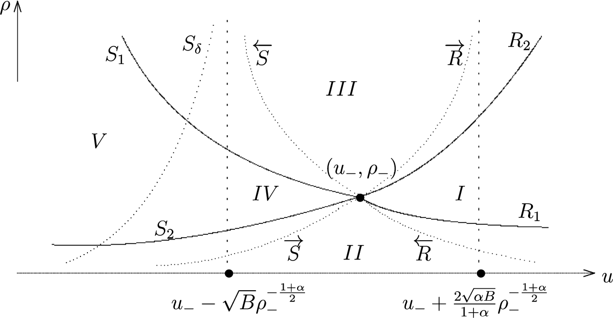
Relationships of elementary wave curves.

From Sections 3 and 4, one can easily observe that, as $γ \to 0$ , the backward (forward) rarefaction wave curve $R_{1}$ ( $R_{2}$ ) of (1.1) approaches to the backward (forward) rarefaction wave curve $\overset{\leftarrow}{R}$ ( $\vec{R}$ ) of (1.4), and the backward (forward) shock wave curve $S_{1}$ ( $S_{2}$ ) of (1.1) tends to the backward (forward) shock wave curve $\overset{\leftarrow}{S}$ ( $\vec{S}$ ) of (1.4) when $α \in (0, 1)$ . See Fig. 4.

6.1. Formation of delta-shock solution as

γ \to 0

We study the formation of the delta shock waves in the limit of solutions of (1.1) and (1.5) in the case $(u_{+}, ρ_{+}) \in V (u_{-}, ρ_{-})$ , that is, $u_{+} + \sqrt{B} ρ_{+}^{- \frac{1 + α}{2}} ⩽ u_{-} - \sqrt{B} ρ_{-}^{- \frac{1 + α}{2}}$ , as the adiabatic exponent $γ \to 0$ .

Lemma 6.1.
When $(u_{+}, ρ_{+}) \in V (u_{-}, ρ_{-})$ , there exists a positive parameter $γ_{0}$ such that $(u_{+}, ρ_{+}) \in S_{1} S_{2} (u_{-}, ρ_{-})$ as $0 < γ < γ_{0}$ .
Proof.
In view of $(u_{+}, ρ_{+}) \in V (u_{-}, ρ_{-})$ , we have $\begin{array}{l} (6.1) & u_{+} + \sqrt{B} ρ_{+}^{- \frac{1 + α}{2}} ⩽ u_{-} - \sqrt{B} ρ_{-}^{- \frac{1 + α}{2}} . \end{array}$ As a result, $\begin{array}{l} {(u_{-} - u_{+})}^{2} ⩾ B (ρ_{+}^{- 1 - α} + ρ_{-}^{- 1 - α} + 2 ρ_{+}^{- \frac{1 + α}{2}} ρ_{-}^{- \frac{1 + α}{2}}) > B (ρ_{+}^{- 1 - α} + ρ_{-}^{- 1 - α} - ρ_{-}^{- 1} ρ_{+}^{α} - ρ_{+}^{- 1} ρ_{-}^{α}), \end{array}$ or written as $\begin{array}{l} (6.2) & {(u_{-} - u_{+})}^{2} > B (\frac{1}{ρ_{-}} - \frac{1}{ρ_{+}}) (\frac{1}{ρ_{-}^{α}} - \frac{1}{ρ_{+}^{α}}) . \end{array}$

All states $(u, ρ)$ connected with $(u_{+}, ρ_{+})$ by a backward shock wave $S_{1}$ or a forward shock wave $S_{2}$ should satisfy $\begin{array}{l} (6.3) & u = u_{-} - \sqrt{(\frac{1}{ρ_{-}} - \frac{1}{ρ}) \cdot (A (ρ^{γ} - ρ_{-}^{γ}) + B (\frac{1}{ρ_{-}^{α}} - \frac{1}{ρ^{α}}))}, ρ > ρ_{-}, \end{array}$ or $\begin{array}{l} (6.4) & u = u_{-} - \sqrt{(\frac{1}{ρ_{-}} - \frac{1}{ρ}) \cdot (A (ρ^{γ} - ρ_{-}^{γ}) + B (\frac{1}{ρ_{-}^{α}} - \frac{1}{ρ^{α}}))}, ρ < ρ_{-} . \end{array}$ When $ρ_{-} = ρ_{+}$ , then $(u_{+}, ρ_{+}) \in S_{1} S_{2} (u_{-}, ρ_{-})$ for any $γ \in (0, 1)$ . While if $ρ_{-} \neq ρ_{+}$ and $(u_{+}, ρ_{+}) \in S_{1} S_{2} (u_{-}, ρ_{-})$ , then from (6.3), (6.4) and Fig. 4, we can deduce that $\begin{array}{l} (6.5) & u_{+} < u_{-} - \sqrt{(\frac{1}{ρ_{-}} - \frac{1}{ρ_{+}}) \cdot (A (ρ_{+}^{γ} - ρ_{-}^{γ}) + B (\frac{1}{ρ_{-}^{α}} - \frac{1}{ρ_{+}^{α}}))}, ρ_{+} > ρ_{-}, \end{array}$ or $\begin{array}{l} (6.6) & u_{+} < u_{-} - \sqrt{(\frac{1}{ρ_{-}} - \frac{1}{ρ_{+}}) \cdot (A (ρ_{+}^{γ} - ρ_{-}^{γ}) + B (\frac{1}{ρ_{-}^{α}} - \frac{1}{ρ_{+}^{α}}))}, ρ_{+} < ρ_{-}, \end{array}$ which yield that $\begin{array}{l} (6.7) & {(u_{-} - u_{+})}^{2} > (\frac{1}{ρ_{-}} - \frac{1}{ρ_{+}}) \cdot (A (ρ_{+}^{γ} - ρ_{-}^{γ}) + B (\frac{1}{ρ_{-}^{α}} - \frac{1}{ρ_{+}^{α}})) . \end{array}$

Since from (6.2) one can obtain that $\begin{array}{l} lim_{γ \to 0} (\frac{1}{ρ_{-}} - \frac{1}{ρ_{+}}) \cdot (A (ρ_{+}^{γ} - ρ_{-}^{γ}) + B (\frac{1}{ρ_{-}^{α}} - \frac{1}{ρ_{+}^{α}})) \\ = B (\frac{1}{ρ_{-}} - \frac{1}{ρ_{+}}) (\frac{1}{ρ_{-}^{α}} - \frac{1}{ρ_{+}^{α}}) < {(u_{-} - u_{+})}^{2}, \end{array}$ it follows that there exists some $γ_{0}$ small enough such that (6.7) holds when $0 < γ < γ_{0}$ . That is to say, $(u_{+}, ρ_{+}) \in S_{1} S_{2} (u_{-}, ρ_{-})$ for $0 < γ < γ_{0}$ . The proof is complete. □

When $0 < γ < γ_{0}$ , the Riemann solution of (1.1) and (1.5) contains a backward shock wave $S_{1}$ plus a forward shock wave $S_{2}$ and the intermediate state $({\tilde{u}}_{}, {\tilde{ρ}}_{})$ , besides two constant states $(u_{\pm}, ρ_{\pm})$ . We then have $\begin{array}{l} (6.8) & S_{1} : \{\begin{matrix} {\tilde{ω}}_{1} = u_{-} - {\tilde{ρ}}_{} \sqrt{\frac{1}{ρ_{-} {\tilde{ρ}}_{} ({\tilde{ρ}}_{} - ρ_{-})} \cdot (A ({\tilde{ρ}}_{}^{γ} - ρ_{-}^{γ}) + B (\frac{1}{ρ_{-}^{α}} - \frac{1}{{\tilde{ρ}}_{}^{α}}))}, \\ {\tilde{u}}_{} = u_{-} - \sqrt{(\frac{1}{ρ_{-}} - \frac{1}{{\tilde{ρ}}_{}}) \cdot (A ({\tilde{ρ}}_{}^{γ} - ρ_{-}^{γ}) + B (\frac{1}{ρ_{-}^{α}} - \frac{1}{{\tilde{ρ}}_{}^{α}}))}, {\tilde{ρ}}_{} > ρ_{-}, \end{matrix} \end{array}$ and $\begin{array}{l} (6.9) & S_{2} : \{\begin{matrix} {\tilde{ω}}_{2} = {\tilde{u}}_{} + ρ_{+} \sqrt{\frac{1}{{\tilde{ρ}}_{} ρ_{+} (ρ_{+} - {\tilde{ρ}}_{})} \cdot (A (ρ_{+}^{γ} - {\tilde{ρ}}_{}^{γ}) + B (\frac{1}{{\tilde{ρ}}_{}^{α}} - \frac{1}{ρ_{+}^{α}}))}, \\ u_{+} = {\tilde{u}}_{} - \sqrt{(\frac{1}{{\tilde{ρ}}_{}} - \frac{1}{ρ_{+}}) \cdot (A (ρ_{+}^{γ} - {\tilde{ρ}}_{}^{γ}) + B (\frac{1}{{\tilde{ρ}}_{}^{α}} - \frac{1}{ρ_{+}^{α}}))}, {\tilde{ρ}}_{} > ρ_{+} . \end{matrix} \end{array}$ Here, ${\tilde{ω}}_{1}$ and ${\tilde{ω}}_{2}$ are the propagation speeds of $S_{1}$ and $S_{2}$ , respectively. Similar to that in Section 5, one has the following lemmas.
Lemma 6.2.
${lim}_{γ \to 0} {\tilde{ρ}}_{} = + \infty$ and* ${lim}_{γ \to 0} {\tilde{ρ}}_{}^{γ} < \frac{ρ_{-} {(u_{-} - u_{+})}^{2} + A}{A}$ .
Proof.
We have, together with (6.8) and (6.9), $\begin{array}{l} u_{-} - u_{+} = & \sqrt{(\frac{1}{ρ_{-}} - \frac{1}{{\tilde{ρ}}_{}}) \cdot (A ({\tilde{ρ}}_{}^{γ} - ρ_{-}^{γ}) + B (\frac{1}{ρ_{-}^{α}} - \frac{1}{{\tilde{ρ}}_{}^{α}}))} \\ (6.10) & + \sqrt{(\frac{1}{{\tilde{ρ}}_{}} - \frac{1}{ρ_{+}}) \cdot (A (ρ_{+}^{γ} - {\tilde{ρ}}_{}^{γ}) + B (\frac{1}{{\tilde{ρ}}_{}^{α}} - \frac{1}{ρ_{+}^{α}}))} . \end{array}$

The desired result can be proved by a similar argument as used in Lemma 5.1. Here, just to be convenient and complete, we show the outline of the proof. If ${lim}_{γ \to 0} {\tilde{ρ}}_{} = \tilde{K} \in (max (ρ_{-}, ρ_{+}), + \infty)$ , then by taking the limit of (6.10) as $γ \to 0$ , one has $\begin{array}{l} u_{-} - u_{+} = \sqrt{B} (\sqrt{(\frac{1}{ρ_{-}} - \frac{1}{\tilde{K}}) (\frac{1}{ρ_{-}^{α}} - \frac{1}{{\tilde{K}}^{α}})} + \sqrt{(\frac{1}{ρ_{+}} - \frac{1}{\tilde{K}}) (\frac{1}{ρ_{+}^{α}} - \frac{1}{{\tilde{K}}^{α}})}), \end{array}$ which leads to, together with (6.1), $\begin{array}{l} \sqrt{B} (\sqrt{(\frac{1}{ρ_{-}} - \frac{1}{\tilde{K}}) (\frac{1}{ρ_{-}^{α}} - \frac{1}{{\tilde{K}}^{α}})} + \sqrt{(\frac{1}{ρ_{+}} - \frac{1}{\tilde{K}}) (\frac{1}{ρ_{+}^{α}} - \frac{1}{{\tilde{K}}^{α}})}) \\ ⩾ \sqrt{B} (ρ_{-}^{- \frac{1 + α}{2}} + ρ_{+}^{- \frac{1 + α}{2}}) = \sqrt{B} (\sqrt{\frac{1}{ρ_{-}} \cdot \frac{1}{ρ_{-}^{α}}} + \sqrt{\frac{1}{ρ_{+}} \cdot \frac{1}{ρ_{+}^{α}}}), \end{array}$ which is not true. Thus, we have ${lim}_{γ \to 0} {\tilde{ρ}}_{} = + \infty$ . Based on this fact, we further obtain from (6.10) that $\begin{array}{l} u_{-} - u_{+} > lim_{γ \to 0} \sqrt{(\frac{1}{ρ_{-}} - \frac{1}{{\tilde{ρ}}_{}}) \cdot (A ({\tilde{ρ}}_{}^{γ} - ρ_{-}^{γ}) + B (\frac{1}{ρ_{-}^{α}} - \frac{1}{{\tilde{ρ}}_{}^{α}}))} . \end{array}$ Then, we have $\begin{array}{l} {(u_{-} - u_{+})}^{2} > \frac{1}{ρ_{-}} (lim_{γ \to 0} A {\tilde{ρ}}_{}^{γ} - A + \frac{B}{ρ_{-}^{α}}) > \frac{1}{ρ_{-}} (lim_{γ \to 0} A {\tilde{ρ}}_{}^{γ} - A), \end{array}$ from which one can solve that ${lim}_{γ \to 0} {\tilde{ρ}}_{}^{γ} < \frac{ρ_{-} {(u_{-} - u_{+})}^{2} + A}{A}$ . We finish the proof. □
Lemma 6.3.
Let* ${lim}_{γ \to 0} {\tilde{u}}_{} = \tilde{σ}$ , then* $\begin{array}{l} (6.11) & lim_{γ \to 0} {\tilde{u}}_{} = lim_{γ \to 0} {\tilde{ω}}_{1} = lim_{γ \to 0} {\tilde{ω}}_{2} = \tilde{σ} \in (u_{+} + \sqrt{α B} ρ_{+}^{- \frac{1 + α}{2}}, u_{-} - \sqrt{α B} ρ_{-}^{- \frac{1 + α}{2}}), \end{array}$
Proof.
Observing Lemma 6.2, from the second equation of (6.8), we have $\begin{array}{l} lim_{γ \to 0} {\tilde{u}}_{} & = u_{-} - lim_{γ \to 0} \sqrt{(\frac{1}{ρ_{-}} - \frac{1}{{\tilde{ρ}}_{}}) \cdot (A ({\tilde{ρ}}_{}^{γ} - ρ_{-}^{γ}) + B (\frac{1}{ρ_{-}^{α}} - \frac{1}{{\tilde{ρ}}_{}^{α}}))} \\ = u_{-} - \sqrt{\frac{1}{ρ_{-}} (lim_{γ \to 0} A ρ_{}^{γ} - A) + \frac{B}{ρ_{-}^{α + 1}}} \\ < u_{-} - \sqrt{α B} ρ_{-}^{- \frac{1 + α}{2}} . \end{array}$

Analogously, from the second equation of (6.9), one has $\begin{array}{l} lim_{γ \to 0} {\tilde{u}}_{} & = u_{+} + lim_{γ \to 0} \sqrt{(\frac{1}{{\tilde{ρ}}_{}} - \frac{1}{ρ_{+}}) \cdot (A (ρ_{+}^{γ} - {\tilde{ρ}}_{}^{γ}) + B (\frac{1}{{\tilde{ρ}}_{}^{α}} - \frac{1}{ρ_{+}^{α}}))} \\ = u_{+} + \sqrt{\frac{1}{ρ_{+}} (lim_{γ \to 0} A ρ_{}^{γ} - A) + \frac{B}{ρ_{+}^{α + 1}}} \\ > u_{+} + \sqrt{α B} ρ_{+}^{- \frac{1 + α}{2}} . \end{array}$ What is more, by a similar analysis as in Lemma 5.2, we can check that ${lim}_{γ \to 0} {\tilde{u}}_{} = {lim}_{γ \to 0} {\tilde{ω}}_{1} = {lim}_{γ \to 0} {\tilde{ω}}_{2} = \tilde{σ}$ . The proof is finished. □

Using Rankine–Hugoniot relation for shock waves, as done in Lemma 5.3, we have
Lemma 6.4.
$\begin{array}{l} (6.12) & lim_{γ \to 0} {\tilde{ρ}}_{} ({\tilde{ω}}_{2} - {\tilde{ω}}_{1}) = \tilde{σ} [ρ] - [ρ u] \end{array}$

and* $\begin{array}{l} (6.13) & lim_{γ \to 0} {\tilde{ρ}}_{} {\tilde{u}}_{} ({\tilde{ω}}_{2} - {\tilde{ω}}_{1}) = \tilde{σ} [ρ u] - [ρ u^{2} - \frac{B}{ρ^{α}}] . \end{array}$

By Lemma 6.4, we can observe that $\begin{matrix} \tilde{σ} [ρ u] - [ρ u^{2} - \frac{B}{ρ^{α}}] = (\tilde{σ} [ρ] - [ρ u]) \cdot \tilde{σ}, \end{matrix}$ from which, and noting that $\tilde{σ} \in (u_{+} + \sqrt{α B} ρ_{+}^{- \frac{1 + α}{2}}, u_{-} - \sqrt{α B} ρ_{-}^{- \frac{1 + α}{2}})$ , we immediately obtain the following result
Lemma 6.5.
For the $\tilde{σ}$ mentioned in this section, we have $\begin{array}{l} \tilde{σ} = \frac{[ρ u] + \sqrt{ρ_{-} ρ_{+} {[u]}^{2} - [ρ] [- \frac{B}{ρ^{α}}]}}{[ρ]} \end{array}$ for $ρ_{-} \neq ρ_{+}$ , and $\begin{matrix} \tilde{σ} = \frac{u_{-} + u_{+}}{2} \end{matrix}$ for $ρ_{-} = ρ_{+}$ .
Remark 6.1.
Lemmas 6.2–6.4 imply that when the adiabatic exponent $γ \to 0$ , the intermediate density ${\tilde{ρ}}_{}$ becomes unbounded, and the velocities ${\tilde{u}}_{}$ and ${\tilde{ω}}_{i}$ ( $i = 1, 2$ ) tend to quantity $\tilde{σ}$ , which uniquely determines the delta-shock solution of (1.4) as the limit of the Riemann solutions of (1.1) and is actually consistent with the generalized Rankine–Hugoniot relation (3.15) and the entropy condition (3.16), as proposed for the delta-shock solution to the generalized Chaplygin gas equations in Section 3.

Finally, by virtue of a similar discussion in Theorem 5.1, we conclude the following result. Theorem 6.1.
Let $(u_{+}, ρ_{+}) \in V (u_{-}, ρ_{-})$ . For any fixed $γ \in (0, 1)$ , suppose that $(u_{γ}, ρ_{γ}) (t, x)$ is a two-shock-wave solution of ( 1.1 ) and ( 1.5 ) for $0 < γ < γ_{0}$ constructed in Section 4 . Then, as $γ \to 0$ , $ρ_{γ}$ and $ρ_{γ} u_{γ}$ converge in the sense of distributions, and the limit functions of $ρ_{γ}$ and $ρ_{γ} u_{γ}$ are the sums of a step function and a Dirac delta function with weights $\begin{array}{l} \frac{t}{\sqrt{1 + {\tilde{σ}}^{2}}} (\tilde{σ} [ρ] - [ρ u]) and \frac{t}{\sqrt{1 + {\tilde{σ}}^{2}}} (\tilde{σ} [ρ u^{2} - \frac{B}{ρ^{α}}]), \end{array}$ respectively, which form the delta-shock solution of the generalized Chaplygin gas equations ( 1.4 ) with the initial data ( 1.5 ).

6.2. Formation of two-rarefaction-wave solution as $γ \to 0$

In what follows, by imposing $γ \to 0$ , we study the formation of the two-rarefaction-wave solution in the solutions of (1.1) and (1.5) when $(u_{+}, ρ_{+}) \in I (u_{-}, ρ_{-})$ for $α \in (0, 1)$ .

Lemma 6.6.
When $(u_{+}, ρ_{+}) \in I (u_{-}, ρ_{-})$ , there exists a positive parameter $γ_{1}$ such that $(u_{+}, ρ_{+}) \in R_{1} R_{2} (u_{-}, ρ_{-})$ as $0 < γ < γ_{1}$ .
Proof.
When $(u_{+}, ρ_{+}) \in I (u_{-}, ρ_{-})$ , we can observe from Fig. 4 together with (3.4) and (3.5) that the following results are true $\begin{array}{l} u_{+} - u_{-} > \frac{2 \sqrt{A γ}}{1 - γ} (ρ_{+}^{\frac{γ - 1}{2}} - ρ_{-}^{\frac{γ - 1}{2}}), \end{array}$ and $\begin{array}{l} u_{+} - u_{-} > - \frac{2 \sqrt{A γ}}{1 - γ} (ρ_{+}^{\frac{γ - 1}{2}} - ρ_{-}^{\frac{γ - 1}{2}}) . \end{array}$ Thus, for $(u_{+}, ρ_{+}) \in I (u_{-}, ρ_{-})$ , we have, $\begin{array}{l} (6.14) & u_{+} - u_{-} > \frac{2 \sqrt{A γ}}{1 - γ} \cdot | ρ_{-}^{\frac{γ - 1}{2}} - ρ_{+}^{\frac{γ - 1}{2}} | . \end{array}$

All states $(u, ρ)$ connected with $(u_{-}, ρ_{-})$ via a backward rarefaction wave $R_{1}$ or a forward rarefaction wave $R_{2}$ satisfy $\begin{array}{l} (6.15) & R_{1} : u = u_{-} - \int_{ρ_{-}}^{ρ} \frac{\sqrt{\frac{A γ}{s^{1 - γ}} + \frac{α B}{s^{α + 1}}}}{s} d s, ρ < ρ_{-}, u > u_{-}, \\ (6.16) & R_{2} : u = u_{-} + \int_{ρ_{-}}^{ρ} \frac{\sqrt{\frac{A γ}{s^{1 - γ}} + \frac{α B}{s^{α + 1}}}}{s} d s, ρ > ρ_{-}, u > u_{-} . \end{array}$ When $ρ_{-} = ρ_{+}$ , the conclusion is obvious. When $ρ_{-} \neq ρ_{+}$ and $(u_{+}, ρ_{+}) \in I (u_{-}, ρ_{-})$ , we can see intuitively from Fig. 4 together with (6.15) and (6.16) that $\begin{array}{l} (6.17) & u_{+} > u_{-} - \int_{ρ_{-}}^{ρ_{+}} \frac{\sqrt{\frac{A γ}{s^{1 - γ}} + \frac{α B}{s^{α + 1}}}}{s} d s, ρ_{+} < ρ_{-} \end{array}$ and $\begin{array}{l} (6.18) & u_{+} > u_{-} + \int_{ρ_{-}}^{ρ_{+}} \frac{\sqrt{\frac{A γ}{s^{1 - γ}} + \frac{α B}{s^{α + 1}}}}{s} d s, ρ_{+} > ρ_{-}, \end{array}$ that is $\begin{array}{l} (6.19) & u_{+} - u_{-} > | \int_{ρ_{-}}^{ρ_{+}} \frac{\sqrt{\frac{A γ}{s^{1 - γ}} + \frac{α B}{s^{α + 1}}}}{s} d s | . \end{array}$ Taking $γ \to 0$ on both sides of (6.19), it becomes nothing but (6.14), which yields that there exists some $γ_{1} > 0$ small enough such that (6.19) holds when $0 < γ < γ_{1}$ . Therefore, it is clear that $(u_{+}, ρ_{+}) \in R_{1} R_{2} (u_{-}, ρ_{-})$ as $0 < γ < γ_{1}$ . The proof is finished. □

When $0 < γ < γ_{1}$ , the Riemann solution of (1.1) and (1.5) contains two rarefaction waves $R_{1}$ and $R_{2}$ with the intermediate state $({\tilde{u}}_{}, {\tilde{ρ}}_{})$ besides two constant states $(u_{\pm}, ρ_{\pm})$ , which is $\begin{array}{l} (6.20) & R_{1} : \{\begin{matrix} ξ = λ_{1}^{α γ} = u - \sqrt{\frac{A γ}{ρ^{1 - γ}} + \frac{α B}{ρ^{α + 1}}}, \\ u = u_{-} - \int_{ρ_{-}}^{ρ} \frac{\sqrt{\frac{A γ}{s^{1 - γ}} + \frac{α B}{s^{α + 1}}}}{s} d s, {\tilde{ρ}}_{} ⩽ ρ ⩽ ρ_{-} \end{matrix} \end{array}$ and $\begin{array}{l} (6.21) & R_{2} : \{\begin{matrix} ξ = λ_{2}^{α γ} = u + \sqrt{\frac{A γ}{ρ^{1 - γ}} + \frac{α B}{ρ^{α + 1}}}, \\ u_{+} = u + \int_{ρ}^{ρ_{+}} \frac{\sqrt{\frac{A γ}{s^{1 - γ}} + \frac{α B}{s^{α + 1}}}}{s} d s, ρ_{+} ⩾ ρ ⩾ {\tilde{ρ}}_{} . \end{matrix} \end{array}$ Here, ${\tilde{ρ}}_{}$ is determined by $\begin{array}{l} (6.22) & u_{+} - u_{-} = \int_{{\tilde{ρ}}_{}}^{ρ_{-}} \frac{\sqrt{\frac{A γ}{s^{1 - γ}} + \frac{α B}{s^{α + 1}}}}{s} d s + \int_{{\tilde{ρ}}_{}}^{ρ_{+}} \frac{\sqrt{\frac{A γ}{s^{1 - γ}} + \frac{α B}{s^{α + 1}}}}{s} d s . \end{array}$ Furthermore, letting $(u_{}, ρ_{}) = {lim}_{γ \to 0} ({\tilde{u}}_{}, {\tilde{ρ}}_{})$ , one has $\begin{array}{l} (6.23) & \{\begin{matrix} u_{} = \frac{u_{+} + u_{-}}{2} + \frac{\sqrt{α B}}{1 + α} (ρ_{+}^{- \frac{1 + α}{2}} - ρ_{-}^{- \frac{1 + α}{2}}), \\ ρ_{} = {(\frac{(1 + α) (u_{+} - u_{-})}{4 \sqrt{α B}} + \frac{1}{2} (ρ_{+}^{- \frac{1 + α}{2}} + ρ_{-}^{- \frac{1 + α}{2}}))}^{- \frac{2}{1 + α}} . \end{matrix} \end{array}$

Letting $γ \to 0$ in (6.20) and (6.21), then for $α \in (0, 1)$ , $R_{1}$ and $R_{2}$ become the backward rarefaction wave $\overset{\leftarrow}{R}$ and the forward rarefaction wave $\vec{R}$ , respectively, as follows $\begin{array}{l} (6.24) & \overset{\leftarrow}{R} : \{\begin{matrix} ξ = λ_{1}^{α} = u - \sqrt{α B} ρ^{- \frac{1 + α}{2}}, \\ u - \frac{2 \sqrt{α B}}{1 + α} ρ^{- \frac{1 + α}{2}} = u_{-} - \frac{2 \sqrt{α B}}{1 + α} ρ_{-}^{- \frac{1 + α}{2}}, ρ_{} < ρ < ρ_{-} \end{matrix} \end{array}$ and $\begin{array}{l} (6.25) & \vec{R} : \{\begin{matrix} ξ = λ_{2}^{α} = u + \sqrt{α B} ρ^{- \frac{1 + α}{2}}, \\ u + \frac{2 \sqrt{α B}}{1 + α} ρ^{- \frac{1 + α}{2}} = u_{+} + \frac{2 \sqrt{α B}}{1 + α} ρ_{+}^{- \frac{1 + α}{2}}, ρ_{} < ρ < ρ_{+} . \end{matrix} \end{array}$

As a conclusion, in this case we have the following Theorem 6.2.
Let* $(u_{+}, ρ_{+}) \in I (u_{-}, ρ_{-})$ . For any fixed $γ \in (0, 1)$ , assume that $(u_{γ}, ρ_{γ})$ is the two-shock-wave solution of ( 1.1 ) and ( 1.5 ) for $0 < γ < γ_{1}$ constructed in Section 4 . Then, as $γ \to 0$ , the limit of the Riemann solution $(u_{γ}, ρ_{γ})$ is expressed as $\begin{array}{l} lim_{γ \to 0} (u_{γ}, ρ_{γ}) (t, x) = \{\begin{matrix} (u_{-}, ρ_{-}), & - \infty < x / t < u_{-} - \sqrt{α B} ρ_{-}^{- \frac{1 + α}{2}}, \\ (u_{}, ρ_{}), & u_{-} - \sqrt{α B} ρ_{-}^{- \frac{1 + α}{2}} ⩽ x / t ⩽ u_{+} + \sqrt{α B} ρ_{+}^{- \frac{1 + α}{2}}, \\ (u_{+}, ρ_{+}), & u_{+} + \sqrt{α B} ρ_{+}^{- \frac{1 + α}{2}} < x / t < + \infty, \end{matrix} \end{array}$ which is just the solution of the generalized Chaplygin gas equations ( 1.4 ) with the initial data ( 1.5 ) containing a nonvacuum state and two rarefaction waves $\overset{\leftarrow}{R}$ and $\vec{R}$ for $0 < α < 1$ .
Remark 6.2.
For the case $γ \in (0, 1)$ and $α = 1$ , since from Remark 3.1 we know that (1.4) corresponds to the Chaplygin gas equations, so one can prove that, as the adiabatic exponent $γ \to 0$ , both the backward (forward) rarefaction wave curve $R_{1}$ ( $R_{2}$ ) and the backward (forward) shock wave curve $S_{1}$ ( $S_{2}$ ) of the extended Chaplygin gas equations (1.1) tend to the backward (forward) contact discontinuity curve of the Chaplygin gas equations (1.4).

7. Conclusion

A new model for extended Chaplygin gas is introduced. By the Riemann problem, the phenomenon of concentration and cavitation as well as the formation of delta shock waves and vacuums are analyzed via using the vanishing exponent limit method. By letting the perturbed exponents tend to zero wholly or partly, two kinds of interesting zero-exponent limit behaviors of solutions are investigated, which to some extent provides us a new angle of view to study the phenomenon of concentration and cavitation. In fact, it is more natural to consider the equations (1.1) with a sour term like [24], or study it in the relativistic version as in [35,39,40], etc. Of course, these may need more complicated calculation, derivation and analysis. We leave them for our future studies.

Footnotes

Acknowledgements

This work was supported by National Natural Science Foundation of China (11501488), Yunnan Applied Basic Research Projects (2018FD015), Scientific Research Foundation Project of Yunnan Education Department (2018JS150), Nan Hu Young Scholar Supporting Program of XYNU, Natural Science Foundation of Hebei Province (A2019105110) and Science and Technology Foundation of Hebei Education Department (QN2018307).

References

H.B.

Benaoum, Accelerated universe from modified Chaplygin gas and tachyonic fluid, arXiv:hep-th/0205140.

Brenier, Solutions with concentration to the Riemann problem for the one-dimensional Chaplygin gas equations, J. Math. Fluid Mech. 7(3) (2005), S326–S331. doi:10.1007/s00021-005-0162-x.

Brenier and

Grenier, Sticky particles and scalar conservation laws, SIAM J. Numer. Anal. 35 (1998), 2317–2328. doi:10.1137/S0036142997317353.

Chaplygin, On gas jets, Sci. Mem. Moscow Univ. Math. Phys. 21 (1904), 1–121.

Chen and

Liu, Formation of delta-shocks and vacuum states in the vanishing pressure limit of solutions to the Euler equations for isentropic fluids, SIAM J. Math. Anal. 34 (2003), 925–938. doi:10.1137/S0036141001399350.

Chen and

Liu, Concentration and cavitation in the vanishing pressure limit of solutions to the Euler equations for nonisentropic fluids, Physica D 189 (2004), 141–165. doi:10.1016/j.physd.2003.09.039.

Cheng and

Yang, Approaching Chaplygin pressure limit of solutions to the Aw–Rascle model, J. Math. Anal. Appl. 416 (2014), 839–854. doi:10.1016/j.jmaa.2014.03.010.

Courant and

K.O.

Friedrichs, Supersonic Flow and Shock Waves, Interscience Publishers Inc., New York, 1948.

Ding,

Witt and

Yin, The global smooth symmetric solution to 2-D full compressible Euler system of Chaplygin gases, J. Differential Equations 258(2) (2015), 445–482. doi:10.1016/j.jde.2014.09.018.

10.

Guo,

Sheng and

Zhang, The two-dimensional Riemann problem for isentropic Chaplygin gas dynamic system, Commun. Pure Appl. Anal. 9 (2010), 431–458. doi:10.3934/cpaa.2010.9.431.

11.

Heydarzade,

Darabi and

Atazadeh, Einstein static universe on the brane supported by extended Chaplygin gas, Astrophys Space Sci. 361(8) (2016), 250. doi:10.1007/s10509-016-2836-7.

12.

Ibrahim,

Liu and

Liu, Concentration of mass in the pressureless limit of Euler equations for power law, Nonlinear Analysis: Real World Applications 47 (2019), 224–235. doi:10.1016/j.nonrwa.2018.10.015.

13.

E.O.

Kahya and

Pourhassan, Observational constraints on the extended Chaplygin gas inflation, Astrophys Space Sci. 353(2) (2014), 677–682. doi:10.1007/s10509-014-2069-6.

14.

Li and

Shao, Delta shocks and vacuum states in vanishing pressure limits of solutions to the relativistic Euler equations for generalized Chaplygin gas, Commun. Pure Appl. Anal. 15(6) (2016), 2373–2400. doi:10.3934/cpaa.2016041.

15.

Li, Note on the compressible Euler equations with zero temperature, Appl. Math. Lett. 14 (2001), 519–523. doi:10.1016/S0893-9659(00)00187-7.

16.

Liu,

Liang and

Yang, Delta shock waves as flux-approximation limit of solutions to the modified Chaplygin gas equations, Acta Applicandae Mathematicae (2019). doi:10.1007/s10440-019-00280-2.

17.

Naji, Extended Chaplygin gas equation of state with bulk and shear viscosities, Astrophys Space Sci. 350(1) (2014), 333–338. doi:10.1007/s10509-013-1714-9.

18.

Naji,

Heydari and

Darabi, New version of viscous Chaplygin gas cosmology with varying gravitational constant, Canadian Journal of Physics 92(12) (2014), 1556–1561. doi:10.1139/cjp-2014-0226.

19.

Pan and

Han, The Aw–Rascle traffic model with Chaplygin pressure, J. Math. Anal. Appl. 401(1) (2013), 379–387. doi:10.1016/j.jmaa.2012.12.022.

20.

B.C.

Paul,

Thakur and

Saha, Observational constraints on extended Chaplygin gas cosmologies, Pramana – J. Phys. 89(2) (2017), 29. doi:10.1007/s12043-017-1417-9.

21.

Pourhassan and

E.O.

Kahya, Extended Chaplygin gas model, Results in Physics 4 (2014), 101–102. doi:10.1016/j.rinp.2014.05.007.

22.

M.R.

Setare, Interacting holographic generalized Chaplygin gas model, Phys. Lett. B 654 (2007), 1–6. doi:10.1016/j.physletb.2007.08.038.

23.

S.F.

Shandarin and

Ya.B.

Zeldovich, The large-scale structure of the universe: Turbulence, intermittency, structures in a self-gravitating medium, Rev. Modern Phys. 61 (1989), 185–220. doi:10.1103/RevModPhys.61.185.

24.

Sheng and

Shao, The vanishing adiabatic exponent limits of Riemann solutions to the isentropic Euler equations for power law with a Coulomb-like friction term, J. Math. Phys. 60(10) (2019), 101504. doi:10.1063/1.5108863.

25.

Sheng and

Shao, Concentration of mass in the pressureless limit of the Euler equations of one-dimensional compressible fluid flow, Nonlinear Analysis: Real World Applications 52 (2020), 103039. doi:10.1016/j.nonrwa.2019.103039.

26.

Sheng,

Wang and

Yin, Delta wave and vacuum state for generalized Chaplygin gas dynamics system as pressure vanishes, Nonlinear Analysis: Real World Applications 22 (2015), 115–128. doi:10.1016/j.nonrwa.2014.08.007.

27.

Sheng and

Zhang, The Riemann problem for transportation equation in gas dynamics, Mem. Am. Math. Soc. 137(654) (1999), 1–77.

28.

Tong and

Shen, The limits of Riemann solutions for the isentropic Euler system with extended Chaplygin gas, Applicable Analysis (2018). doi:10.1080/00036811.2018.1469009.

29.

Tsien, Two dimensional subsonic flow of compressible fluids, J. Aeron. Sci. 6 (1939), 399–407. doi:10.2514/8.916.

30.

von Karman, Compressibility effects in aerodynamics, J. Aeron. Sci. 8 (1941), 337–365. doi:10.2514/8.10737.

31.

Wang, The Riemann problem for one dimensional generalized Chaplygin gas dynamics, J. Math. Anal. Appl. 403(2) (2013), 434–450. doi:10.1016/j.jmaa.2013.02.026.

32.

Weinan,

Yu.G.

Rykov and

Ya.G.

Sinai, Generalized variational principles, global weak solutions and behavior with random initial data for systems of conservation laws arising in adhesion particle dynamics, Comm. Math. Phys. 177 (1996), 349–380. doi:10.1007/BF02101897.

33.

Yang and

Wang, Delta-shocks and vacuum states in the vanishing pressure limit of solutions to the isentropic Euler equations for modified Chaplygin gas, J. Math. Anal. Appl. 413 (2014), 800–820. doi:10.1016/j.jmaa.2013.12.025.

34.

Yang and

Wang, Concentration in vanishing pressure limit of solutions to the modified Chaplygin gas equations, J. Math. Phys. 57(11) (2016), 111504. doi:10.1063/1.4967299.

35.

Yang and

Zhang, Pressure and flux-approximation to the isentropic relativistic Euler equations for modified Chaplygin gas, J. Math. Phys. 60(7) (2019), 071502. doi:10.1063/1.5093531.

36.

Yin and

Song, Vanishing pressure limits of Riemann solutions to the isentropic relativistic Euler system for Chaplygin gas, J. Math. Anal. Appl. 411 (2014), 506–521. doi:10.1016/j.jmaa.2013.09.050.

37.

Zhang, Concentration in the flux approximation limit of Riemann solutions to the extended Chaplygin gas equations, J. of Math. (PRC) 39(4) (2019), 504–528.

38.

Zhang,

Pang and

Wang, Concentration and cavitation in the vanishing pressure limit of solutions to the generalized Chaplygin Euler equations of compressible fluid flow, Eur. J. Mech. B Fluids 78 (2019), 252–262. doi:10.1016/j.euromechflu.2019.103515.

39.

Zhang,

Sun and

Lin, Solutions with concentration and cavitation to the Riemann problem for the isentropic relativistic Euler system for the extended Chaplygin gas, Open Mathematics 17(1) (2019), 220–241. doi:10.1515/math-2019-0017.

40.

Zhang and

Yang, Limits of solutions to the relativistic Euler equations for modified Chaplygin gas by flux approximation, Acta Applicandae Mathematicae (2019). doi:10.1007/s10440-019-00286-w.

Concentration in the zero-exponent limit of solutions to the isentropic Euler equations for extended Chaplygin gas

Abstract

Keywords

1. Introduction

2. Delta shocks and vacuums for the zero-pressure flow

Lemma 3.1 ([31]).

5.1. Limit behavior of Riemann solutions as α , γ → 0

Footnotes

Acknowledgements

References

5.1. Limit behavior of Riemann solutions as $α, γ \to 0$