We investigate the stability of a one-dimensional wave equation with non smooth localized internal viscoelastic damping of Kelvin–Voigt type and with boundary or localized internal delay feedback. The main novelty in this paper is that the Kelvin–Voigt and the delay damping are both localized via non smooth coefficients. Under sufficient assumptions, in the case that the Kelvin–Voigt damping is localized faraway from the tip and the wave is subjected to a boundary delay feedback, we prove that the energy of the system decays polynomially of type . However, an exponential decay of the energy of the system is established provided that the Kelvin–Voigt damping is localized near a part of the boundary and a time delay damping acts on the second boundary. While, when the Kelvin–Voigt and the internal delay damping are both localized via non smooth coefficients near the boundary, under sufficient assumptions, using frequency domain arguments combined with piecewise multiplier techniques, we prove that the energy of the system decays polynomially of type . Otherwise, if the above assumptions are not true, we establish instability results.
Viscoelastic materials feature intermediate characteristics between purely elastic and purely viscous behaviors, i.e., they display both behaviors when undergoing deformation. In wave equations, when the viscoelastic controlling parameter is null, the viscous property vanishes and the wave equation becomes a pure elastic wave equation. However, time delays arise in many applications and practical problems like physical, chemical, biological, thermal and economic phenomena, where an arbitrary small delay may destroy the well-posedness of the problem and destabilize it. Actually, it is well-known that the simplest delay equations of parabolic type,
or hyperbolic type
with a delay parameter , are not well-posed. Their instability is due to the existence of a sequence of initial data remaining bounded, while the corresponding solutions go to infinity in an exponential manner at a fixed time (see [19,29]).
The stabilization of a wave equation with Kelvin–Voigt type damping and internal or boundary time delay has attracted the attention of many authors in the last five years. Indeed, in 2016 Messaoudi et al. studied the stabilization of a wave equation with global Kelvin–Voigt damping and internal time delay in the multidimensional case (see [35]), and they obtained an exponential stability result. In the same year, Nicaise et al. in [38] considered the multidimensional wave equation with localized Kelvin–Voigt damping and mixed boundary condition with time delay. They obtained an exponential decay of the energy regarding that the damping is acting on a neighborhood of part of the boundary via a smooth coefficient. Also, in 2018, Anikushyn et al. in [18] considered the stabilization of a wave equation with global viscoelastic material subjected to an internal strong time delay where a global exponential decay rate was obtained. Thus, it seems to us that there are no previous results concerning the case of wave equations with internal localized Kelvin–Voigt type damping and boundary or internal time delay, especially in the absence of smoothness of the damping coefficient even in the one-dimensional case. So, we are interested in studying the stability of elastic wave equation with local Kelvin–Voigt damping and with boundary or internal time delay (see Systems (1.1) and (1.2)).
This paper investigates the study of the stability of a string with Kelvin–Voigt type damping localized via a non-smooth coefficient and subjected to a localized internal or boundary time delay. Indeed, in the first part of this paper, we study the stability of elastic wave equation with local Kelvin–Voigt damping, boundary feedback and time delay term at the boundary, i.e., we consider the following system
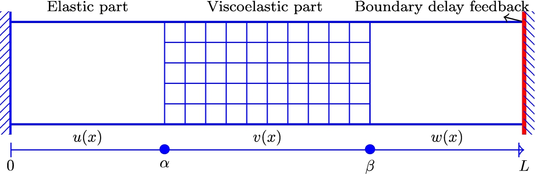
where L, τ, and are strictly positive constant numbers, is a non zero real number and the initial data belongs to a suitable space. Here and , with is the characteristic function of the interval . We assume that there exist strictly positive constant numbers , , , such that . In fact, here we will consider two cases. In the first case, we divide the bar into 3 pieces; the first piece is an elastic part, the second piece is the viscoelastic part and in the third piece, the time delay feedback is effective at the ending point of the piece, i.e., we consider the case (see Fig. 1). While, in the second case, we divide the bar into 2 pieces; the first piece is the viscoelastic part and in the second piece the time delay feedback is effective at the ending point of the piece, i.e., we consider the case (see Fig. 2). Remark, here, in both cases, the Kelvin–Voigt damping is effective on a part of the piece and the time delay is effective at L. Regarding System (1.1), when , and , in the case where the delay is only effective at 1, Datko in [16] (see Example 3.5) proved that System (1.1) is unstable for an arbitrary small value of τ. Later, when and in the absence of delay (i.e., ), they proved in [2,8] that the energy of System (1.1) is polynomially stable. Indeed, when and , the stability of System (1.1) is still an open problem. In this paper, we assume that
We consider two cases. Case one, if (see Fig. 1), then using the semigroup theory of linear operators and a result obtained by Borichev and Tomilov, we show that the energy of System (1.1) has a polynomial decay rate of type . Case two, if (see Fig. 2), then using the semigroup theory of linear operators and a result obtained by Huang and Prüss, we prove an exponential decay of the energy of System (1.1).
K-V damping is acting localized in the internal of the body and time delay feedback is effective at L.
K-V damping is acting localized near the boundary of the body and time delay feedback is effective at L.
In the second part of this paper, we study the stability of the elastic wave equation with local Kelvin–Voigt damping and local internal time delay. This system takes the following form
where L, τ and are strictly positive constant numbers, is a non zero real number and the initial data belongs to a suitable space. Here , and , with is the characteristic function of the interval . We assume that there exist strictly positive constant numbers , , such that . In fact, here we will divide the bar into 2 pieces; the first piece is an elastic part, while in the second piece the Kelvin–Voigt damping and the time delay are effective (see Fig. 3). So, the Kelvin–Voigt damping and the time delay are effective on . Regarding System (1.2), in the absence of delay (i.e., ), they proved in [2,3,40] that the energy of System (1.2) is polynomially stable. Indeed, when , the stability of System (1.2) is still an open problem. In this paper, we assume that
By using the semigroup theory of linear operators and a result obtained by Borichev and Tomilov, we show that the energy of the System (1.2) has a polynomial decay rate of type . Moreover, when , , if , we show that there exists a sequence of arbitrary small (and large) delays such that instabilities occur.
Local internal K-V damping and local internal delay feedback.
In the literature, let us consider the one-dimensional wave equation with time delay
For the stability of System (1.3), what are the conditions on , , and τ? In 1985, Datko et al. in [17] considered System (1.3) with and , where they added an internal term and the internal damping . The system is given by the following:
where the delay parameter τ is strictly positive, and . So, the above system models a string having a boundary feedback with delay at the free end. They showed that if , then System (1.4) is strongly stable for all small enough delays. However, if , then there exists an open set D dense in , such that for all τ in D, System (1.4) admits exponentially unstable solutions. Moreover, in the absence of delay in System (1.4) (i.e., ) and , , its energy decays exponentially to zero under the condition (see [15]). In 1990, Datko in [16] (see Example 3.5) considered System (1.3) with and , also he added the strong internal damping . The system is given by the following:
where τ, κ and δ are strictly positive constant numbers. Even in the presence of the strong damping , without any other damping, He proved that System (1.5) is unstable for an arbitrary small value of τ. In 2006, Xu et al. in [49] considered System (1.3) with and , where they added the boundary term . The system is given by the following:
where τ, κ and μ are strictly positive constant numbers. The above system represents a wave equation that is fixed at one end and subjected to a boundary control input possessing a partial time delay of weight at the other end. They proved the following stability results:
In 2008, Guo and Xu in [22] studied the stabilization of a wave equation in the case where it is affected by a boundary control and output observation suffering from time delay. The system is given by the following:
where w is the control and y is the output observation. Using the separation principle, the authors proved that the above delayed system is exponentially stable. In 2010, Gugat in [21] considered System (1.3) with , if and if . The problem is described by the following system
where τ and L are strictly positive constant numbers, while λ is a real number. When with and , Gugat proved that the above system is exponentially stable. The result in [21] has been improved by J. Wang et al. in [47]. Indeed, in 2011, J. Wang et al. in [47] considered System (1.3) with , . The system is given by the following:
where τ is a strictly positive constant number and κ is a real number. They showed that if the delay is equal to even multiples of the wave propagation time, then the above closed loop system is exponentially stable under sufficient and necessary conditions for κ. Else, if the delay is an odd multiple of the wave propagation time, thus the closed loop system is unstable. In 2013, H. Wang et al. in [46], studied System (1.6) under the feedback control law provided that the weight of the feedback with delay is a real β and that of the feedback without delay is a real α. They found a feedback control law that stabilizes exponentially the system for any , by modifying the velocity feedback into the form , where f is a linear functional. Finally, in 2017, Xu et al. in [48], considered System (1.3) with , , also they added the internal term . The system is given by the following:
where , and κ is real number. Based on the idea of Lyapunov functional, they proved an exponential stability result of the above system under a certain relationship between α and κ.
Going to the multidimensional case, the stability of the wave equation with time delay has been studied in [4,5,9,18,35,37,38,42]. In 2006, Nicaise and Pignotti in [37] studied the multidimensional wave equation considering two cases. The first case concerns a wave equation with boundary feedback and a delay term at the boundary
The second case concerns a wave equation with internal feedback and a delayed velocity term (i.e., an internal delay) and a mixed Dirichlet-Neumann boundary condition
In both systems, be is considered to be an open bounded set with a boundary Γ of class , Γ is divided into two parts and , i.e., , such that and . Moreover, denotes the outer unit normal vector to the point , is the partial derivative, is the time delay, and are strictly positive constant numbers. Under the assumption that the weight of the feedback with delay is smaller than that without delay , they obtained an exponential decay of the energy of both Systems (1.7) and (1.8). On the contrary, if the previous assumption does not hold (i.e., ), they found a sequence of delays for which the energy of some solutions does not tend to zero (see [13] for the treatment of Problem (1.8) in more general abstract form). In 2009, Nicaise et al. in [39] studied System (1.7) in the one-dimensional case where the delay time τ is a function depending on time and they established an exponential stability result under the condition that the derivative of the decay function is upper bounded by a constant and assuming that . In 2010, Ammari et al. in [9] studied the wave equation with interior delay damping and dissipative undelayed boundary condition. The system is given by the following:
where ; , is an open bounded set with a boundary Γ, Γ is divided into two closed parts and , i.e., , such that and . Moreover, , and . Under the condition that satisfies the Γ-condition introduced in [30], they proved that System (1.9) is uniformly asymptotically stable whenever the delay coefficient is sufficiently small. In 2012, Pignotti in [42] considered the wave equation with internal distributed time delay and local damping in a bounded and smooth domain ; , with a boundary Γ. The system is given by the following:
where κ real, and . System (1.10) shows that the damping is localized, indeed, it acts on a neighborhood of a part of the boundary of Ω. Under the assumption that , the author established an exponential decay rate. Later, in 2016, Messaoudi et al. in [35] considered the stabilization of the following wave equation with strong time delay
where Ω is a bounded and regular domain of ; , with a boundary Γ, represents the time delay, and are real numbers such that . They obtained an exponential stability result. In addition, in the same year, Nicaise et al. in [38] studied the multidimensional wave equation with localized Kelvin–Voigt damping and mixed boundary condition with time delay
where is an open bounded set with a boundary Γ of class , Γ is divided into two open parts and , i.e., , such that and , . Moreover, denotes the outer unit normal vector to the point , is the partial derivative, is the time delay, κ is a real number, and on ω such that is an open neighborhood of . Under an appropriate geometric condition on and assuming that , , they proved an exponential decay of the energy of System (1.11). In 2017, Ammari and Gerbi in [6] considered an interior stabilization problem for the wave equation with dynamic boundary delay. The system is given by the following:
where ; is an open bounded set with a boundary Γ, Γ is divided into two closed parts and , i.e., , such that and . Moreover, denotes the outer unit normal vector to the point , is the partial derivative, is the time delay, a and μ are positive numbers. They proved some stability results under the choice of the damping operator. The proof of the main result is based on a frequency domain method and combines a contradiction argument with the multiplier technique to carry out a special analysis for the resolvent. Finally, in 2018, Anikushyn et al. in [18] considered an initial boundary value problem for a viscoelastic wave equation subjected to a strong time localized delay in a Kelvin–Voigt type. The system is given by the following:
where is an open bounded Lipschitz domain set with a boundary Γ of class , Γ is divided into two open parts and , i.e., , such that and . Moreover, denotes the outer unit normal vector to the point , is the partial derivative, is the time delay, and , , , are positive real numbers. Under appropriate conditions on the coefficients, a global exponential decay rate is obtained. We can also mention that Ammari et al. in [10] considered the stabilization problem for an abstract equation with delay and a Kelvin–Voigt damping in 2015. The system is given by the following:
for an appropriate class of operator and . Using the frequency domain approach, they obtained an exponential stability result. Finally, the transmission problem of a wave equation with global or local Kelvin–Voigt damping and without any time delay was studied by many authors in the one-dimensional case (see [1–3,20,23–25,27,31,33,40,44]) and in the multidimensional case (see [7,26,32,36,45,50]) and polynomial and exponential stability results were obtained. In addition, the stability of wave equations on a tree with local Kelvin–Voigt damping has been studied in [8]. Thus, as we confirmed in the beginning, the case of wave equations with localized Kelvin–Voigt type damping and boundary or internal time delay; as in our Systems (1.1) and (1.2), where the damping is acting in a non-smooth region is still an open problem. The aim of the present paper consists in studying the stability of the Systems (1.1) and (1.2).
This paper is organized as follows: In Section 2, we study the stability of System (1.1). Indeed, in Section 2.1, we consider the case . Under hypothesis (H), first, we prove the well-posedness of System (1.1). Next, we prove the strong stability of the system in the lack of the compactness of the resolvent of the generator. Then, we establish a polynomial energy decay rate of type (see Theorem 2.7). In addition, in Section 2.2, we consider the case and we prove the exponential stability of System (1.1) (see Theorem 2.14). In Section 3, we study the stability of System (1.2). Under hypothesis (H1), first, we prove the well-posedness of System (1.2). Next, we establish a polynomial energy decay rate of type (see Theorem 3.2). Finally, when , , and , we show that System (1.1) is unstable (see Theorem 3.8).
Wave equation with local Kelvin–Voigt damping and with boundary delay feedback
This section is devoted to our first aim, which is to study the stability of a wave equation with localized Kelvin–Voigt damping and boundary delay feedback (see System (1.1)). For this aim, like in [37], we introduce the auxiliary unknown
Thus, Problem (1.1) is equivalent to
Under assumption (H), let us define the energy of a solution of System (2.1) as
Multiplying the first equation of (2.1) by , integrating over with respect to x, then using integration by parts and the boundary conditions in (2.1) at and at , we get
Multiplying the second equation of (2.1) by η, integrating over with respect to ρ, then using the fact that , we get
Adding (2.3) and (2.4), we get
For all , we have
Inserting the above equation in (2.5), we get
Under assumption (H), we can easily check that there exists a strictly positive number p satisfying
such that
so that the energies of the strong solutions satisfy . Hence, System (2.1) is dissipative in the sense that its energy is non increasing with respect to the time t.
For studying the stability of System (2.1), we consider two cases. In Section 2.1, we consider the first case, when the Kelvin–Voigt damping is localized in the internal of the body, i.e., . While in Section 2.2, we consider the second, when the Kelvin–Voigt damping is localized near the boundary of the body, i.e., .
Wave equation with local Kelvin–Voigt damping far from the boundary and with boundary delay feedback
In this subsection, we assume that there exist α and β such that , in this case, the Kelvin–Voigt damping is localized in the internal of the body (see Fig. 1). For this aim, we denote the longitudinal displacement by U and this displacement is divided into three parts
In this case, System (2.1) is equivalent to the following system
with the following boundary and transmission conditions
and with the following initial conditions
where the initial data belongs to a suitable Hilbert space. So, using (2.2), the energy of System (2.8)–(2.10) is given by
Similar to (2.5) and (2.6), we get
where p is defined in (2.7). Thus, under hypothesis (H), the System (2.8)–(2.10) is dissipative in the sense that its energy is non increasing with respect to the time t. Now, we are in position to prove the existence and uniqueness of the solution of our system.
Well-posedness of the problem
We start this part by formulating System (2.8)–(2.10) as an abstract Cauchy problem. For this aim, let us define
The Hilbert space is equipped with the norm:
Also, it is easy to check that the space is Hilbert space over equipped with the norm:
Moreover, by Poincaré inequality we can easily verify that there exists depending on , , , α, β and L, such that
We now define the Hilbert energy space by
equipped with the following inner product
where and . We use to denote the corresponding norm. We define the linear unbounded operator by:
and for all
If is a regular solution of System (2.8)–(2.10), then we transform this system into the following initial value problem
where . We now use semigroup approach to establish well-posedness result for the System (2.8)–(2.10). According to Lumer–Phillips theorem (see [41]), we need to prove that the operator is m-dissipative in . Therefore, we prove the following proposition.
Under hypothesis (H), the unbounded linear operatoris m-dissipative in the energy space.
For all , we have
Here Re is used to denote the real part of a complex number. Using integration by parts in the above equation, we get
On the other hand, since , we have
Inserting the above equation in (2.12), we get
Under hypothesis (H), we easily check that there exists such that
By Young’s inequality, we get
Inserting the above inequality in (2.13), we get
From the construction of p, we have
Therefore, from (2.14), we get
which implies that is dissipative. Now, let us go on with maximality. Let we look for solution of the equation
Equivalently, we consider the following system
In addition, we consider the following boundary conditions
From (2.16)–(2.18) and the fact that , it is clear that . Next, from (2.18), (2.26) and the fact that , we get
From the above equation and Equation (2.22), we can determine
It is clear that and . Inserting the above equation in (2.25), then System (2.16)–(2.26) is equivalent to
Let . Multiplying Equations (2.28), (2.29), (2.30) by , , , integrating over , and respectively, taking the sum, then using integration by parts, we get
From the fact that , we have
Inserting the above equation in (2.34), then using (2.27) and (2.31)–(2.33), we get
We can easily verify that the left-hand side of (2.35) is a bilinear continuous coercive form on , and the right-hand side of (2.35) is a linear continuous form on . Then, using Lax–Milgram theorem, we deduce that there exists unique solution of the variational Problem (2.35). Using standard arguments, we can show that . Finally, by setting , , and and by applying the classical elliptic regularity we deduce that is the solution of Equation (2.15). To conclude, we need to show the uniqueness of U. So, let be a solution of (2.15) with , then we directly deduce that and that satisfies Problem (2.35) with zero in the right hand side. This implies that , in other words, ker and 0 belongs to the resolvent set of . Then, by contraction principle, we easily deduce that for sufficiently small . This, together with the dissipativeness of , imply that is dense in and that is m-dissipative in (see Theorems 4.5, 4.6 in [41]). The proof is thus complete. □
Thanks to Lumer–Philips theorem (see [41]), we deduce that generates a -semigroup of contractions in and therefore Problem (2.8)–(2.10) is well-posed. Then we have the following result:
Under hypothesis (H), for any, Problem (
2.11
) admits a unique weak solution,, such that. Moreover, if, then.
Strong stability
Our main result in this part is the following theorem.
Under hypothesis (H), the-semigroup of contractionsis strongly stable on the Hilbert spacein the sense that
For the proof of Theorem 2.4, according to Theorem A.2 in the Appendix, we need to prove that the operator has no pure imaginary eigenvalues and contains only a countable number of continuous spectrum of . The argument for Theorem 2.4 relies on the subsequent lemmas.
Under hypothesis (H), for, we haveis injective, i.e.,,.
From Proposition 2.2, we have . We still need to show the result for . Suppose that there exists a real number and such that
First, similar to Equation (2.14), we have
Thus,
Next, writing (2.36) in a detailed form gives
From (2.44) and (2.37), we get
Combining (2.37) with (2.39), we get that
Thus,
Inserting the above result in (2.42), then taking into consideration (2.39), we obtain
From the definition of and using (2.45)–(2.47), we get
Combining (2.38) with (2.41) and (2.40) with (2.43) and using the above equation as boundary conditions, we get
Thus,
Combining (2.48) with (2.38) and (2.40), we obtain
Finally, from the above result, (2.45), (2.47) and (2.48), we get that . The proof is thus complete. □
Under hypothesis (H), for, we haveis surjective, i.e.,,.
Since , we still need to show the result for . For any and , we prove the existence of solution for the following equation
Equivalently, we consider the following problem
with the following boundary conditions
It follows from (2.55), (2.59) and (2.51) that
Inserting (2.49)–(2.51) and (2.60) in (2.52)–(2.59) and deriving (2.50) with respect to x, we get
Let . Multiplying Equations (2.61), (2.62), (2.63) by , , , integrating over , and respectively, taking the sum, then using integration by parts, we get
From the fact that , we have
Inserting the above equation in (2.68), then using (2.64)–(2.67), we get
where
and
such that
Let be the dual space of . We define the operators A, and by
such that
Our aim is to prove that the operator A is an isomorphism. For this aim, we proceed the proof in three steps.
Step 1. In this step, we prove that the operator is an isomorphism. For this aim, according to (2.70), we have
We can easily verify that is a bilinear continuous coercive form on . Then, by Lax–Milgram lemma, the operator is an isomorphism.
Step 2. In this step, we prove that the operator is compact. First, for , we introduce the Hilbert space by
Thus by trace theorem, there exists , such that
Now, according to (2.70), we have
Then, by using (2.71), we get
where . Therefore, for all there exists , such that
which implies that
Finally, using the compactness embedding from into we deduce that is compact.
From steps 1 and 2, we get that the operator is a Fredholm operator of index zero 0. Consequently, by Fredholm alternative, proving the operator A is an isomorphism reduces to proving .
Step 3. In this step, we prove that the . For this aim, let , i.e.,
Equivalently,
Then, we find that
Therefore, the vector define by belongs to and we have . Thus, , therefore by Lemma 2.5, we get , this implies that , and , so .
Therefore, from step 3 and Fredholm alternative, we get that the operator A is an isomorphism. It easy to see that the operator F is continuous form on . Consequently, Equation (2.69) admits a unique solution . Thus, using (2.49)–(2.51), (2.60) and a classical regularity arguments, we conclude that admits a unique solution . The proof is thus complete. □
From Lemma 2.5, we have that the operator has no pure imaginary eigenvalues and by Lemma 2.6, for all . Therefore, the closed graph theorem implies that . Thus, we get the conclusion by applying Theorem A.2 of Arendt and Batty. The proof is thus complete. □
Polynomial stability
In this part, we will prove the polynomial stability of System (2.8)–(2.10). Our main result in this part is the following theorem.
Under hypothesis (H), for all initial data, there exists a constantindependent ofsuch that the energy of System (
2.8
)–(
2.10
) satisfies the following estimation
From Lemma 2.5 and Lemma 2.6, we have seen that , then for the proof of Theorem 2.7, according to Theorem A.4 (part (ii)) in the Appendix, we need to prove that
We will argue by contradiction. Indeed, suppose there exists
such that
and there exists sequence , such that
In case that , we will check condition (2.73) by finding a contradiction with such as . From now on, for simplicity, we drop the index n. By detailing Equation (2.75), we get the following system
Remark that, since , we have the following boundary conditions
and
The proof of Theorem 2.7 is divided into several lemmas.
Under hypothesis (H), for all, the solutionof Equations (
2.76
)–(
2.82
) satisfies the following asymptotic behavior estimations
Taking the inner product of (2.75) with in , then using the fact that is uniformly bounded in , we get
Now, under hypothesis (H), similar to Equation (2.14), we get
where
Therefore, from (2.89), we get (2.85) and (2.86). Next, from (2.77), (2.85) and the fact that in , we get (2.87). Finally, from (2.84) and (2.86), we obtain (2.88). The proof is thus complete. □
Under hypothesis (H), for all, the solutionof Equations (
2.76
)–(
2.82
) satisfies the following asymptotic behavior estimation
It follows from (2.82) that
By using Cauchy Schwarz inequality, we get
Integrating over with respect to ρ, then using (2.86) and the fact that in , we get
hence, we get (2.90). Thus, the proof of the lemma is complete. □
Under hypothesis (H), for all, the solutionof Equations (
2.76
)–(
2.82
) satisfies the following asymptotic behavior estimations
Multiplying Equation (2.81) by and integrating over , we get
From (2.78), we deduce that
Inserting the above result in (2.94), then using the fact that ϕ, are uniformly bounded in and , converge to zero in gives
Taking the real part in the above equation, then using integration by parts, we get
Inserting (2.86) and (2.88) in the above equation, we get
hence, we get (2.91) and (2.92). Finally, from (2.83) and (2.92), we obtain (2.93). The proof is thus complete. □
Under hypothesis (H), for all, the solutionof Equations (
2.76
)–(
2.82
) satisfies the following asymptotic behavior estimations
Let such that
where and are strictly positive constant numbers independent from λ. The proof is divided into three steps.
Step 1. In this step, we prove the following asymptotic behavior estimate
First, from (2.77), we have
Multiplying the above equation by and integrating over , then taking the real part, we get
using integration by parts in the left hand side of above equation, we get
Consequently, we obtain
On the other hand, we have
Inserting the above equation in (2.99), then using (2.87) and the fact that in , we get
hence, we get (2.98).
Step 2. In this step, we prove the following asymptotic behavior estimate
First, multiplying (2.80) by and integrating over , then taking the real part, we get
using integration by parts in the left-hand side of the above equation, we get
Consequently, we obtain
Now, using Cauchy Schwarz inequality, Equations (2.85), (2.87) and the fact that in in the right hand side of above equation, we get
On the other hand, we have
Inserting the above equation in (2.101), then using Equations (2.85) and (2.87), we get
hence, we get (2.100).
Step 3. In this step, we prove the asymptotic behavior estimations of (2.95)–(2.97). First, multiplying (2.80) by and integrating over , then taking the real part, we get
consequently,
From the fact that z is uniformly bounded in and in , we get
On the other hand, using integration by parts and (2.85), (2.87), we get
Inserting the above equation and Equation (2.103) in (2.102), we get
Now, for or , we have
Substituting the above equation in (2.104), we get
Next, inserting Equations (2.98) and (2.100) in the above inequality, we obtain
consequently,
Since , by choosing , we get
hence, we get (2.95). Finally, inserting (2.95) in (2.98) and (2.100) and using the first asymptotic estimate of (2.93), we get (2.96) and (2.97). The proof is thus complete. □
An example about g, we can take to get
Also, we can take
Under hypothesis (H), for all, the solutionof Equations (
2.76
)–(
2.82
) satisfies the following asymptotic behavior estimations
Multiplying Equation (2.79) by and integrating over , we get
From (2.76), we deduce that
Inserting the above result in (2.106), then using the fact that , y are uniformly bounded in and , converge to zero in gives
Taking the real part in the above equation, then using integration by parts, we get
Inserting the boundary conditions (2.83) at in the above equation to get
Finally, substituting (2.96) and (2.97) in the above equation, we obtain (2.105). The proof is thus complete. □
From Lemma 2.8, Lemma 2.9, Lemma 2.10, Lemma 2.11 and Lemma 2.13, we get
To obtain , we need , so we choose as the optimal value. Hence, we obtain that which contradicts (2.74). Therefore, the energy of System (2.8)–(2.10) satisfies estimation (2.72) for all initial data . The proof is thus complete. □
Wave equation with local Kelvin–Voigt damping near the boundary and boundary delay feedback
In this subsection, we study the stability of System (2.1), but in the case that the Kelvin–Voigt damping is near the boundary, i.e., and (see Fig. 2). For this aim, we denote the longitudinal displacement by U and this displacement is divided into two parts
In this case, System (2.1) is equivalent to the following system
Similar to Section 2.1, we define
where the Hilbert space is equipped with the norm:
Moreover, it is easy to check that the space is Hilbert space over equipped with the norm:
In addition, by Poincaré inequality we can easily verify that there exists depending on , , β and L, such that
We now define the Hilbert energy space by
equipped with the following inner product
where and . We use to denote the corresponding norm. We define the linear unbounded operator by:
and for all
If is a regular solution of System (2.107), then we transform this system into the following initial value problem
where . Note that is dense in and that for all , we have
where p is defined in (2.7). Consequently, under hypothesis (H), the system becomes dissipative. We can easily adapt the proof in Section 2.1.1 to prove the well-posedness of System (2.108).
Under hypothesis (H), for all initial data, the System (
2.107
) is exponentially stable.
According to Theorem A.4 (part (i)) in the Appendix, we have to check if the following conditions hold,
and
First, we can easily adapt the proof in Section 2.1.2 to prove the strong stability (condition (2.110)) of System (2.107). Next, we will prove (2.111) by a contradiction argument. Indeed, suppose there exists
such that
and there exists sequence , such that
We will check condition (2.111) by finding a contradiction with such as . From now on, for simplicity, we drop the index n. By detailing Equation (2.113), we get the following system
Remark that, since , we have the following boundary conditions
Taking the inner product of (2.113) with in , then using (2.109), hypothesis (H) and the fact that is uniformly bounded in , we obtain
Taking (2.114), then using the first asymptotic estimate of (2.121) and the fact that in , we get
Taking the first asymptotic estimate of (2.120), then using the second and the third asymptotic estimates of (2.121), we obtain
Similarly as in Lemma 2.9, with , taking (2.118), then using the second and the third asymptotic estimates of (2.121), we obtain
Similarly as in Lemma 2.10, with , multiplying Equation (2.117) by and integrating over , after that using the fact that , then using the fact that ϕ, are uniformly bounded in and , converge to zero in gives
Taking the real part in the above equation, then using integration by parts, Equation (2.123) and the second asymptotic estimate of (2.121), we obtain
hence, we get
Inserting the third and the fourth asymptotic estimates of (2.125) in (2.119), we get
Similar to step 3 of Lemma 2.11, with and , multiplying (2.116) by and integrating over , taking the real part, then using the fact that z is uniformly bounded in and in , we get
On the other hand, using integration by parts, the fact that , and Equations (2.121)–(2.122), (2.126), we get
Inserting (2.128) in (2.127), we get
Finally, from (2.122), (2.124), (2.125) and (2.129), we get , which contradicts (2.112). Therefore, (2.111) holds and the result follows from Theorem A.4 (part (i)) in the Appendix. The proof is thus complete. □
Wave equation with local internal Kelvin–Voigt damping and local internal delay feedback
In this section, we study the stability of System (1.2). We assume that there exist α such that , in this case, the Kelvin–Voigt damping and the time delay feedback are locally distributed near the boundary (see Fig. 3). For this aim, we denote the longitudinal displacement by U and this displacement is divided into two parts
Furthermore, like in [37], we introduce the auxiliary unknown
In this case, System (1.2) is equivalent to the following system
with the Dirichlet boundary conditions
with the following transmission conditions
and with the following initial conditions
Under assumption (H1), let us define the energy of a solution of System (3.1)–(3.6) as
Multiplying (3.1), (3.2) and by , and , integrating over , and respectively, taking the sum, then using integration by parts and the boundary conditions in (3.4)–(3.5), we get
Uuing Young’s inequality for the third term in the right, we get
Under assumption (H1), the energies of the strong solutions satisfy . Hence, the System (3.1)–(3.6) is dissipative in the sense that its energy is non increasing with respect to the time t.
Well-posedness of the problem
We start this part by formulating System (3.1)–(3.6) as an abstract Cauchy problem. For this aim, let us define
The spaces , and are obviously a Hilbert spaces over equipped respectively with the norms
and
In addition by Poincaré inequality, we can easily verify that there exist and depending on , , α and L, such that
Let us define the energy Hilbert space by
equipped with the following inner product
where and . We use to denote the corresponding norm. We define the linear unbounded operator by:
and for all
If is a regular solution of System (3.1)–(3.6), then we transform this system into the following initial value problem
where . We now use semigroup approach to establish well-posedness result for the System (3.1)–(3.6). We prove the following proposition.
Under hypothesis (H1), the unbounded linear operatoris m-dissipative in the energy space.
For all , we have
Using integration by parts in the above equation, we get
Since , we have
Substituting the above boundary conditions in (3.8), then using Young’s inequality, we get
hence under hypothesis (H1), we get
which implies that is dissipative. We next prove the m-dissipative of . Let . We should prove that there exists a unique solution of the equation
Equivalently, we consider the following system
In addition, we consider the following boundary conditions
From (3.10)–(3.11) and the fact that , we obtain . Next, from (3.11), (3.17) and the fact that , we get
From the above equation and Equation (3.14), we can determine
Since , and , then it is clear that .
Our next aim is to prove that System (3.12)–(3.13) with boundary conditions (3.15)–(3.16) has a unique solution , in addition . For this aim, let . Multiplying Equations (3.12) and (3.13) by and , integrating over and respectively, taking the sum, then using integration by parts, we get
From the fact that , we have
Inserting the above equation in (3.19), then using (3.11), (3.16) and (3.18), we get
We can easily verify that the left-hand side of (3.20) is a bilinear continuous coercive form on and the right-hand side of (3.20) is a linear continuous form on . Then, using Lax–Milgram theorem, we deduce that there exists unique solution of the variational Problem (3.20). Using (3.11), (3.18) and (3.20) once we obtain
Since , , and is a unique solution of (3.21), then by classical elliptic regularity we deduce that the unique solution of (3.20) satisfies . On the other hand, using (3.21) once more we obtain
In (3.22) by choosing , we get a.e. Returning (3.22), there remains
Since is arbitrary, we deduce that . Then, System (3.12)–(3.13) with boundary conditions (3.15)–(3.16) has a unique solution and . Thus, we deduce that there exists a unique solution of the equation . Thus, 0 belongs to the resolvent set of . Then, by contraction principle, we easily deduce that for sufficiently small . This, together with the dissipativeness of , imply that is dense in and that is m-dissipative in (see Theorems 4.5, 4.6 in [41]). The proof is thus complete. □
Thanks to Lumer–Philips theorem (see [41]), we deduce that generates a -semigroup of contractions in and therefore Problem (3.1)–(3.6) is well-posed.
Polynomial stability
The main result in this subsection is the following theorem.
Under hypothesis (H1), for all initial data, there exists a constantindependent ofsuch that the energy of System (
3.1
)–(
3.6
) satisfies the following estimation
According to Theorem A.4 (part (ii)) in the Appendix, we have to check if the following conditions hold:
and
The next proposition is a technical result to be used in the proof of Theorem 3.2 given below.
Under hypothesis (H1), let, such thatThat isThen, we have the following inequalityIn addition, if, then we haveHere and below we denote bya positive constant number independent of λ.
For the proof of Proposition 3.3, we need the following lemmas.
Under hypothesis (H1), the solutionof Equation (
3.25
) satisfies the following estimateswhere
First, taking the inner product of (3.25) with U in , then using hypothesis (H1), arguing in the same way as (3.9), we obtain
hence we get (3.33). Next, from (3.27), (3.33) and the fact that , we obtain
therefore we get (3.34). Now, from (3.30) and using the fact that (i.e., ), we obtain
consequently, we obtain
Inserting (3.33) in the above equation, then using the fact that , we obtain
hence we get (3.35). On the other hand, from (3.37), we get
From the above equation and (3.33), we obtain
Finally, from (3.33), (3.34) and the above inequality, we get
hence we get (3.36). The proof is thus complete. □
Under hypothesis (H1), for alland, the solutionof Equation (
3.25
) satisfies the following estimatesandwhere
First, from Equation (3.27), we have
Multiplying the above equation by , integrating over and taking the real parts, then using integration by parts and the fact that , we get
On the other hand, for all and , we have
Inserting the above equation in (3.40), then using (3.34) and the fact that , we get
hence we get (3.38). Next, multiplying Equation (3.29) by , integrating over and taking the real parts, then using integration by parts, we get
Consequently, we have
On the other hand, for all and , we have
Inserting the above equation in (3.41), we get
Substituting (3.36) in the above equation, then using the fact that
we get
hence we get (3.39). The proof is thus complete. □
Under hypothesis (H1), for all, the solutionof Equation (
3.25
) satisfies the following estimatewhere
First, multiplying Equation (3.28) by , integrating over and taking the real parts, then using integration by parts, we get
From (3.26), we deduce that
Inserting the above result in (3.43), then using integration by parts, we get
consequently, we get
Using Cauchy Schwarz inequality, we get
On the other hand, since , we have
Substituting (3.45) and (3.46) in (3.44), we obtain
Inserting (3.38) and (3.39) with in the above estimation, we get
In the above equation, using the fact that
we get
hence, we get (3.42). The proof is thus complete. □
Under hypothesis (H1), for alland, the solutionof Equation (
3.25
) satisfies the following estimatesandsuch thatwhere
First, from (3.34), (3.35) and (3.42), we get
hence we get (3.47). Next, multiplying (3.29) by and integrating over , then taking the real part, then using integration by parts and the fact that , we get
consequently,
Using Cauchy Schwarz inequality, we have
From (3.33) and (3.36), we get
Inserting (3.50) and the above estimation in (3.49), we get
Now, for all , , we get
Substituting (3.38) and (3.39) in the above estimation, we obtain
where
Finally, inserting the above equation in (3.51), we get
hence we get (3.48). The proof is thus complete. □
We now divide the proof into two steps:
Step 1. In this step, we prove the asymptotic behavior estimate (3.31). Taking , , and in Lemma 3.7, we get
In the above equation, using the fact that
we get
and
Inserting (3.52) in (3.53), we get
hence we get (3.31).
Step 2. In this step, we prove the asymptotic behavior estimate (3.32). Let such that . In this case, taking , , and in Lemma 3.7, we get
and
From the fact that , we get
Therefore, from the above inequality and (3.55), we get
In Estimation (3.56), using the fact that
we get
Inserting (3.57) in (3.54), then using the fact that
we get
hence we get estimate (3.32). The proof is thus complete. □
First, we will prove (3.23). Remark that it has been proved in Proposition 3.1 that . Now, suppose (3.23) is not true, then there exists such that . According to Lemma A.3 in the Appendix, there exists
with as , and , such that
We will check (3.23) by finding a contradiction with such as . According to Equation (3.31) in Proposition 3.3 with , and , we obtain
as , we get , which contradicts . Thus, condition (3.23) holds true. Next, we will prove (3.24) by a contradiction argument. Suppose there exists
with without affecting the result, such that , and and there exists a sequence , such that
We will check (3.24) by finding a contradiction with such as . According to Equation (3.32) in Proposition 3.3 with , , and , we get
as , we get , which contradicts . Thus, condition (3.24) holds true. The result follows from Theorem A.4 (part (ii)) in the Appendix. The proof is thus complete. □
Instability
In this part, we restrict our analysis to the case , . Then, System (1.2) becomes
where κ, L, τ and are strictly positive constant numbers, is a non zero real number and the initial data belongs to a suitable space. Let us define the energy of a solution of System (3.58) as
The main result in this subsection is the following theorem.
If (H1) does not hold (i.e.,), then there exist a sequence of arbitrary small (or large) delays, and solutions of Problem (
3.58
) corresponding to these delays, such that their standard energy does not tend to 0.
We seek a solution of (3.58) in the form
Substituting (3.59) in (3.58), we obtain
Consequently,
Assume that
Remark that, since we are considering the case , then there exist λ, τ such that (3.61) holds. Substituting (3.61) in (3.60), we get
We distinguish two cases.
Case 1. If , then we take
We can easily check that and are solutions of (3.61) and (3.62). Inserting (3.63) in (3.59), we get that (3.58) admits solutions in the form
with is a set of time delays that become arbitrarily small (or large) for suitable choices of the indices . Furthermore, we have
Thus, the energy is constant and strictly positive. Therefore, we have instability phenomena for a sequence of arbitrarily small or large time delays.
Case 2. If , then we take
We can easily check that and are solutions of (3.61) and (3.62). Inserting the above equation in (3.59), we get that (3.58) admits solutions in the form
with is a set of time delays that become arbitrarily small (or large) for suitable choices of the indices . On the other hand, we have
Therefore, the energy is constant and strictly positive. Thus, we have instability phenomena for a sequence of arbitrarily small or large time delays. The proof is thus complete. □
Footnotes
Notions of stability and theorems used
We introduce here the notions of stability that we encounter in this work.
For proving the strong stability of the -semigroup , we will recall two methods, the first result obtained by Arendt and Batty in [11].
The second one is a classical method based on Arendt and Batty theorem and the contradiction argument (see page 25 in [34]).
We now recall the following standard result which is stated in a comparable way (see [28,43] for part (i) and [12,12,14] for part (ii)).
Acknowledgements
The authors would like to thank the anonymous referees for their valuable comments and useful suggestions.
Rayan Nasser would like to thank the CNRS for its support in the framework of PHC CEDRE project untitled Modélisation mathématiques de mécanismes énergétiques dans les tumeurs cérébrales et contrôle de certains systèmes distribués.
References
1.
M.Akil, I.Issa and A.Wehbe, Stability results of an elastic/viscoelastic transmission problem of locally coupled waves with non smooth coefficients. arXiv: Analysis of PDEs, 2020.
2.
M.Alves, J.M.Rivera, M.Sepúlveda and O.V.Villagrán, The lack of exponential stability in certain transmission problems with localized Kelvin–Voigt dissipation, SIAM Journal on Applied Mathematics74(2) (2014), 345–365. doi:10.1137/130923233.
3.
M.Alves, J.M.Rivera, M.Sepúlveda, O.V.Villagrán and M.Z.Garay, The asymptotic behavior of the linear transmission problem in viscoelasticity, Mathematische Nachrichten287(5–6) (2013), 483–497. doi:10.1002/mana.201200319.
4.
K.Ammari and B.Chentouf, Asymptotic behavior of a delayed wave equation without displacement term, Zeitschrift für angewandte Mathematik und Physik68(5) (2017). doi:10.1007/s00033-017-0865-x.
5.
K.Ammari and B.Chentouf, On the exponential and polynomial convergence for a delayed wave equation without displacement, Applied Mathematics Letters86 (2018), 126–133. doi:10.1016/j.aml.2018.06.021.
6.
K.Ammari and S.Gerbi, Interior feedback stabilization of wave equations with dynamic boundary delay, Zeitschrift für Analysis und ihre Anwendungen36(3) (2017), 297–327. doi:10.4171/zaa/1590.
7.
K.Ammari, F.Hassine and L.Robbiano, Stabilization for the wave equation with singular Kelvin–Voigt damping, Archive for Rational Mechanics and Analysis236(2) (2020), 577–601. doi:10.1007/s00205-019-01476-4.
8.
K.Ammari, Z.Liu and F.Shel, Stability of the wave equations on a tree with local Kelvin–Voigt damping, Semigroup Forum100(2) (2020), 364–382. doi:10.1007/s00233-019-10064-7.
9.
K.Ammari, S.Nicaise and C.Pignotti, Feedback boundary stabilization of wave equations with interior delay, Systems & Control Letters59(10) (2010), 623–628. doi:10.1016/j.sysconle.2010.07.007.
10.
K.Ammari, S.Nicaise and C.Pignotti, Stability of an abstract-wave equation with delay and a Kelvin–Voigt damping, Asymptotic Analysis95(1–2) (2015), 21–38. doi:10.3233/ASY-151317.
11.
W.Arendt and C.J.K.Batty, Tauberian theorems and stability of one-parameter semigroups, Trans. Amer. Math. Soc.306(2) (1988), 837–852. doi:10.2307/2000826.
12.
C.J.K.Batty and T.Duyckaerts, Non-uniform stability for bounded semi-groups on Banach spaces, Journal of Evolution Equations8(4) (2008), 765–780. doi:10.1007/s00028-008-0424-1.
13.
E.M.A.Benhassi, K.Ammari, S.Boulite and L.Maniar, Feedback stabilization of a class of evolution equations with delay, Journal of Evolution Equations9(1) (2009), 103–121. doi:10.1007/s00028-009-0004-z.
14.
A.Borichev and Y.Tomilov, Optimal polynomial decay of functions and operator semigroups, Math. Ann.347(2) (2010), 455–478. doi:10.1007/s00208-009-0439-0.
15.
G.Chen, Energie decay estimates and exact boundary value controllability for the wave equation in a bounded domain, J. Math. Pures Appl.9(58) (1979), 249–273.
16.
R.Datko, Two questions concerning the boundary control of certain elastic systems, Journal of Differential Equations92(1) (1991), 27–44. doi:10.1016/0022-0396(91)90062-e.
17.
R.Datko, J.Lagnese and M.Polis, An example of the effect of time delays in boundary feedback stabilization of wave equations, in: 1985 24th IEEE Conference on Decision and Control, IEEE, 1985. doi:10.1109/cdc.1985.268529.
18.
H.Demchenko, A.Anikushyn and M.Pokojovy, On a Kelvin–Voigt viscoelastic wave equation with strong delay, SIAM Journal on Mathematical Analysis51(6) (2019), 4382–4412. doi:10.1137/18m1219308.
19.
M.Dreher, R.Quintanilla and R.Racke, Ill-posed problems in thermomechanics, Applied Mathematics Letters22(9) (2009), 1374–1379. doi:10.1016/j.aml.2009.03.010.
20.
M.Ghader and A.Wehbe, A transmission problem for the Timoshenko system with one local Kelvin–Voigt damping and non-smooth coefficient at the interface, Computational and Applied Mathematics (2020), To appear in.
21.
M.Gugat, Boundary feedback stabilization by time delay for one-dimensional wave equations, IMA Journal of Mathematical Control and Information27(2) (2010), 189–203. doi:10.1093/imamci/dnq007.
22.
B.-Z.Guo and C.-Z.Xu, Boundary output feedback stabilization of a one-dimensional wave equation system with time delay, IFAC Proceedings Volumes41(2) (2008), 8755–8760. doi:10.3182/20080706-5-kr-1001.01480.
23.
F.Hassine, Stability of elastic transmission systems with a local Kelvin–Voigt damping, European Journal of Control23 (2015), 84–93. doi:10.1016/j.ejcon.2015.03.001.
24.
F.Hassine, Energy decay estimates of elastic transmission wave/beam systems with a local Kelvin–Voigt damping, International Journal of Control89(10) (2016), 1933–1950. doi:10.1080/00207179.2015.1135509.
25.
F.Hassine and N.Souayeh, Stability for coupled waves with locally disturbed Kelvin–Voigt damping. arXiv: Analysis of PDEs, 2019.
26.
A.Hayek, S.Nicaise, Z.Salloum and A.Wehbe, A transmission problem of a system of weakly coupled wave equations with Kelvin–Voigt dampings and non-smooth coefficient at the interface, SeMA Journal (2020). doi:10.1007/s40324-020-00218-x.
27.
F.Huang, On the mathematical model for linear elastic systems with analytic damping, SIAM Journal on Control and Optimization26(3) (1988), 714–724. doi:10.1137/0326041.
28.
F.L.Huang, Characteristic conditions for exponential stability of linear dynamical systems in Hilbert spaces, Ann. Differential Equations1(1) (1985), 43–56.
29.
P.Jordan, W.Dai and R.Mickens, A note on the delayed heat equation: Instability with respect to initial data, Mechanics Research Communications35(6) (2008), 414–420. doi:10.1016/j.mechrescom.2008.04.001.
30.
J.-L.Lions, Contrôlabilité Exacte, Perturbations et Stabilisation de Systèmes Distribués. Tome 1, Recherches en Mathématiques Appliquées, Vol. 8, Masson, Paris, 1988.
31.
K.Liu and Z.Liu, Exponential decay of energy of the Euler–Bernoulli beam with locally distributed Kelvin–Voigt damping, SIAM Journal on Control and Optimization36(3) (1998), 1086–1098. doi:10.1137/s0363012996310703.
32.
K.Liu and B.Rao, Exponential stability for the wave equations with local Kelvin–Voigt damping, Zeitschrift für angewandte Mathematik und Physik57(3) (2006), 419–432. doi:10.1007/s00033-005-0029-2.
33.
Z.Liu and Q.Zhang, Stability of a string with local Kelvin–Voigt damping and non smooth coefficient at interface, SIAM Journal on Control and Optimization54(4) (2016), 1859–1871. doi:10.1137/15m1049385.
34.
Z.Liu and S.Zheng, Semigroups Associated with Dissipative Systems, Chapman & Hall/CRC Research Notes in Mathematics, Vol. 398, Chapman & Hall/CRC, Boca Raton, FL, 1999.
35.
S.A.Messaoudi, A.Fareh and N.Doudi, Well posedness and exponential stability in a wave equation with a strong damping and a strong delay, Journal of Mathematical Physics57(11) (2016), 111501. doi:10.1063/1.4966551.
36.
R.Nasser, N.Noun and A.Wehbe, Stabilization of the wave equations with localized Kelvin–Voigt type damping under optimal geometric conditions, Comptes Rendus Mathematique357(3) (2019), 272–277. doi:10.1016/j.crma.2019.01.005.
37.
S.Nicaise and C.Pignotti, Stability and instability results of the wave equation with a delay term in the boundary or internal feedbacks, SIAM Journal on Control and Optimization45(5) (2006), 1561–1585. doi:10.1137/060648891.
38.
S.Nicaise and C.Pignotti, Stability of the wave equation with localized Kelvin–Voigt damping and boundary delay feedback, Discrete and Continuous Dynamical Systems – Series S9(3) (2016), 791–813. doi:10.3934/dcdss.2016029.
39.
S.Nicaise, J.Valein and E.Fridman, Stability of the heat and of the wave equations with boundary time-varying delays, Discrete and Continuous Dynamical Systems – Series S2(3) (2009), 559–581. doi:10.3934/dcdss.2009.2.559.
40.
H.P.Oquendo, Frictional versus Kelvin–Voigt damping in a transmission problem, Mathematical Methods in the Applied Sciences40(18) (2017), 7026–7032. doi:10.1002/mma.4510.
41.
A.Pazy, Semigroups of Linear Operators and Applications to Partial Differential Equations, Applied Mathematical Sciences., Vol. 44, Springer-Verlag, New York, 1983. doi:10.1007/978-1-4612-5561-1.
42.
C.Pignotti, A note on stabilization of locally damped wave equations with time delay, Systems & Control Letters61(1) (2012), 92–97. doi:10.1016/j.sysconle.2011.09.016.
43.
J.Prüss, On the spectrum of -semigroups, Trans. Amer. Math. Soc.284(2) (1984), 847–857. doi:10.2307/1999112.
44.
J.E.M.Rivera, O.V.Villagran and M.Sepulveda, Stability to localized viscoelastic transmission problem, Communications in Partial Differential Equations43(5) (2018), 821–838. doi:10.1080/03605302.2018.1475490.
45.
L.Tebou, A constructive method for the stabilization of the wave equation with localized Kelvin–Voigt damping, Comptes Rendus Mathematique350(11–12) (2012), 603–608. doi:10.1016/j.crma.2012.06.005.
46.
H.Wang and G.Q.Xu, Exponential stabilization of 1-d wave equation with input delay, Wseas Transactions on Mathematics12(10) (2013), 1001–1013.
47.
J.-M.Wang, B.-Z.Guo and M.Krstic, Wave equation stabilization by delays equal to even multiples of the wave propagation time, SIAM Journal on Control and Optimization49(2) (2011), 517–554. doi:10.1137/100796261.
48.
Y.Xie and G.Xu, Exponential stability of 1-d wave equation with the boundary time delay based on the interior control, Discrete & Continuous Dynamical Systems – S10(3) (2017), 557–579. doi:10.3934/dcdss.2017028.
49.
G.Q.Xu, S.P.Yung and L.K.Li, Stabilization of wave systems with input delay in the boundary control, in: ESAIM: Control, Optimisation and Calculus of Variations, Vol. 12, 2006, pp. 770–785. doi:10.1051/cocv:2006021.
50.
Q.Zhang, Polynomial decay of an elastic/viscoelastic waves interaction system, Zeitschrift für angewandte Mathematik und Physik69(4) (2018). doi:10.1007/s00033-018-0981-2.