A hardware efficient intra-cortical neural decoding approach based on spike train temporal information

Abstract

Motor intention decoding is one of the most challenging issues in brain machine interface (BMI). Despite several important studies on accurate algorithms, the decoding stage is still processed on a computer, which makes the solution impractical for implantable applications due to its size and power consumption. This study aimed to provide an appropriate real-time decoding approach for implantable BMIs by proposing an agile decoding algorithm with a new input model and implementing efficient hardware. This method, unlike common ones employed firing rate as input, used a new input space based on spike train temporal information. The proposed approach was evaluated based on a real dataset recorded from frontal eye field (FEF) of two male rhesus monkeys with eight possible angles as the output space and presented a decoding accuracy of 62%. Furthermore, a hardware architecture was designed as an application-specific integrated circuit (ASIC) chip for real-time neural decoding based on the proposed algorithm. The designed chip was implemented in the standard complementary metal-oxide-semiconductor (CMOS) 180 nm technology, occupied an area of 4.15 mm ${}^{2}$ , and consumed 28.58 $\mu$ W @1.8 V power supply.

Keywords

Implantable brain machine interface real-time intra-cortical neural signal decoding spike train temporal information hardware implementation

1. Introduction

Brain machine interface (BMI) employs neural information to create a communication channel between the brain and an external device [1, 2, 3, 4, 5, 7, 8, 9, 6, 10]. As a result of the more preferable temporal and spatial resolution of the modern intracranial recording devices [5, 11], intra-cortical BMIs are desirable candidates to convert complex neural data into commands [12, 13, 14, 15, 16, 17]. In the design of BMI systems for intra-cortical decoding the definition of a suitable model for the sequences of the neural spike is essential [18]. Most methods employ rate coding hypothesis as their model, in which the considered information is encoded into the number of spikes existing in a time bin known as firing rate [19, 20]. In traditional decoding methods, a time-independent linear or non-linear method such as Wiener filter or Wiener cascade algorithm is adopted to map the firing rate of just one moment to its related movement without considering its time variations [21, 22, 23]. Another approach is support vector machine (SVM) which is one of the most well-known methods in machine learning algorithms [24, 25, 26, 27]. Finally, another approach for accurate decoding is Feedforward neural network which maps the inputs to the output space by some sequential layers. Although the computational complexity of these methods is low due to their simplicity, the accuracy of the estimation is insufficient in many applications [28, 29, 30, 31, 32].

Other approaches employ some algorithms such as recurrent neural networks (RNN) to consider long-term firing rates of the neurons as well as the current input to estimate the output space [33]. Since these complex architectures process temporal information stored by the past data, they can provide higher decoding accuracy but with higher computational cost [34]. long short-term memory (LSTM) [35], Elman [36], and gated recurrent unite (GRU) neural networks [37] are some common algorithms in this category.

Moreover, state space model (SSM) is another widely used decoding method [38, 39, 40] which is applicable for closed-loop systems. Another approach proposed in [41] uses spike distance [42] and firing rate as the inputs to consider temporal information in the algorithm. This approach can provide more accurate results.However, more complicated computations are expected for more inputs. Although most of the aforementioned methods improve the performance of the decoding process, the main section of the algorithms is still conducted on a computer that is power-hungry and not easily portable, which can lead to an impractical approach for long-term use [43]. While by the on-chip implementation of an algorithm, by the reduction in size and power consumption, the computing device would be perfect as an implantable processor [35]. Despite the cited benefit, few studies have implemented decoding algorithms on-chip. For instance, a decoder algorithm based on LSTM architecture was implemented on a Field-Programmable Gate Array (FPGA) [35]. In other research a probabilistic neural network (PNN) is implemented on a FPGA to decode the data recorded from rats performing a lever-pressing task [44]. Additionally, an Extreme Learning Machine algorithm was implemented for neural decoding by combining analog and digital designing [43].

In this paper, firstly instead of firing rate, the actual spikes would be directly utilized; after some discussion about the new model and the achieved results, it would be shown that not only it is more hardware-friendly, but also as a result of employing the actual spikes from the past to the current moment the outputs of the algorithm are more accurate. Then, the SVM algorithm is selected as the best candidate to process the proposed inputs with an acceptable decoding accuracy and hardware implementation costs at the same time. Finally, based on the proposed algorithm, efficient hardware architecture is designed and implemented as an ASIC decoder processor chip, which is suitable for implantable BMIs. In summary the contributions of our method are highlighted as follows:

•
New input space is introduced which reduces computational complexity.
•
New hardware is designed to minimize area and power required for an implantable BMI.
•
Very accurate result is achieved by a relatively simple algorithm which was feasible only by complicated methods before.

Figure 1.
Routine followed for each trial.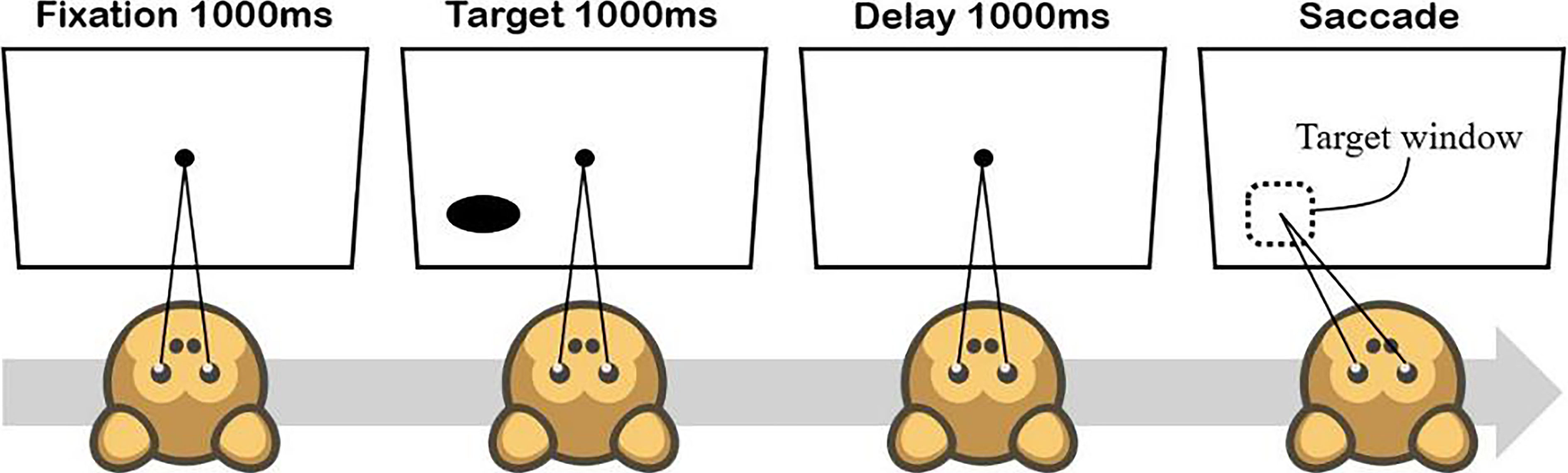

Figure 2.
Considering the spikes in narrow time bins and constructing the patterns of ones and zeros corresponding to spike occurrences or non-occurrences.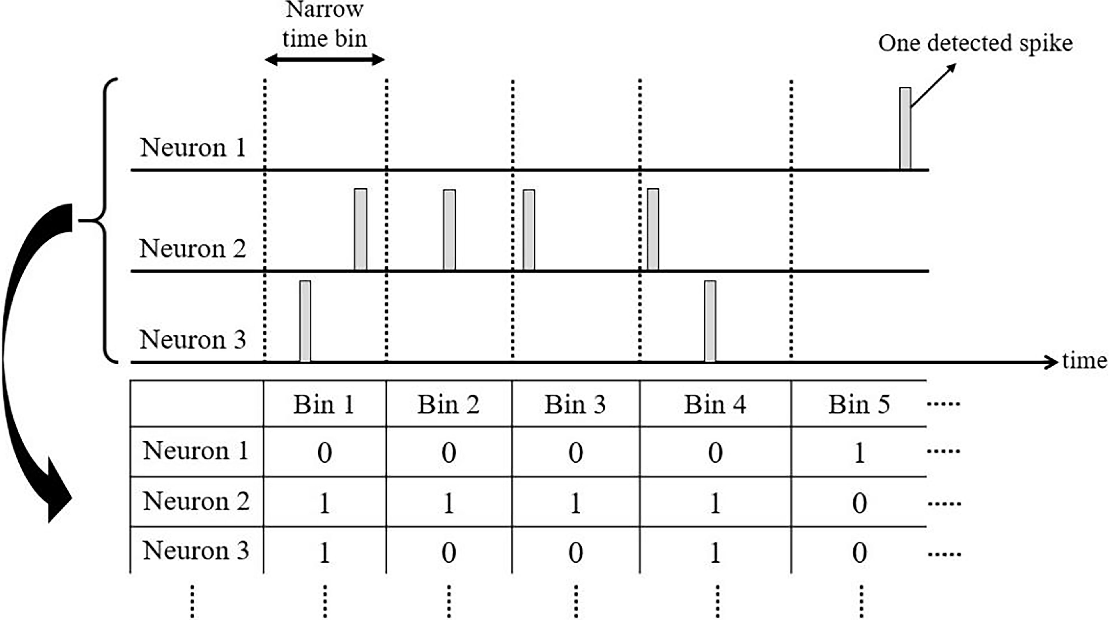

The rest of this paper is organized as follows. In Section 2, the dataset used for both training and testing phases is specified. Then, the proposed model for the cited inputs is presented in Section 3. Next, in Section 4, several algorithms are analyzed with respect to accuracy and computational complexity aspects to select a candidate for processing the proposed inputs. Based on the chosen method, an algorithm as well as an optimized hardware implementation are introduced in Sections 5 and 6. Moreover, the results and the discussions related to our tests are reported in Section 7. Finally, our conclusion is provided in Section 8.
2. Data specification

The data employed for training and evaluating the proposed approach in this paper was the recorded neural activity from the Frontal Eye Field (FEF) of two male rhesus monkeys (machaca mulatta) during a memory-guided saccade task and it is sourced from the recorded data in [24]. For each monkey, a multisite linear array electrode with a head post was surgically implanted, which made simultaneous recording from 16 channels possible. As illustrated in Fig. 1, the monkeys were trained to start each trial by looking at a fixation point on a monitor located 28.5 cm in front of their eyes. Then, a visual target appeared in one of the eight different angles (0, 45, 90, 135, 180, 225, 270, and 315 degrees). The targets remained on the screen for only one-second. Finally, the monkey had to saccade to the remembered location after one-second delay. If the monkey successfully followed the cited procedure and saccaded to the correct angle, he would receive a drop of juice as his reward after 792 recorded trials, the spikes were sorted in 32 neurons and used as the data by utilizing the algorithm presented in [24].

3. Inputs model

Most decoding algorithms employ the firing rate as the input to decode motor cortex commands [45, 46]. Despite the simplicity and acceptable accuracy of firing rate in this type of decoding, there is considerably more information in temporal patterns of spike trains, especially in decoding visual and auditory cortex neural signals [47, 48, 49]. Some studies have shown that employing temporal patterns information is effective for increasing decoding accuracy even for the motor cortex by utilizing RNN [50] or spike train distance [41]. The present study considers temporal information in the decoding process with an efficient computational complexity.

Figure 3.

Routine of merging time bins to reduce the input space.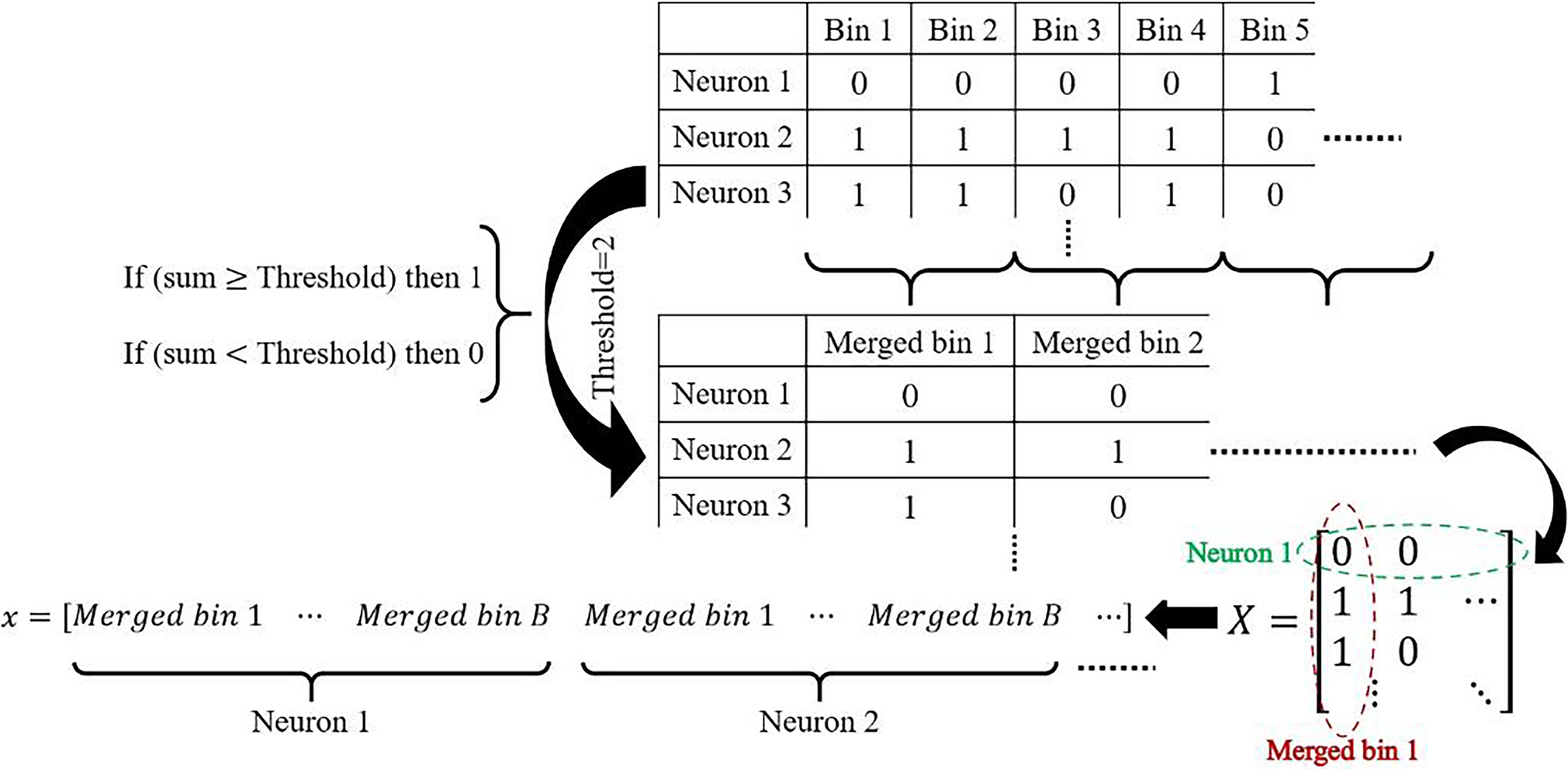

In the suggested approach, the time bin for considering the spikes is narrower to allow just one spike can be maximally detected. As shown in Fig. 2, the patterns of ones and zeros corresponding to spikes occurrence or non-occurrence are constructed by time-shifting the narrow bin and employing it for all neurons. The collected data shown in Fig. 2 is very informative. The comparison between the fires in each bin for each neuron indicates the time of the spike occurrences. Furthermore, when it is compared with the other neurons, it indicates when the other neurons would have spikes with respect to the considered neuron, which in other words is temporal data. Additionally, when the firing rate of each neuron is under consideration, it can be calculated by the density of ones from some successive bins based on Fig. 2. Therefore, the table has more valuable information when it is compared with the methods which only employ firing rates.

On the other hand, two major issues are raised by employing the defined input space in its current format and RNN algorithms for processing the temporal information. Based on our experiments, a noticeable number of sequence bins should be used for accurate decoding, which would lead to a too complicated mapping function between input and output space. In addition, RNN methods are typically too complicated for hardware implementation. Thus, an algorithm with lower computational complexity should be utilized.

The last difficulty is discussed in the next section, and a solution is proposed for the first one in this section. As shown in Fig. 3, it is suggested to merge some successive bins to create a new bin for decreasing the input space to a much reasonable one with smaller dimensions, which are called the merged bin. If the sum of the fires in the merged sequence bins is above a pre-defined threshold, the fire of the related merged bin would be considered one. Otherwise, it would be mapped to zero. In this way, the data is collected in a $N\times B$ matrix with $N$ neurons and $B$ merged bins, which is called $X$ in this paper (Fig. 3). In other words, an approximation is applied which has still preserved temporal information but has at least two benefits and one downside. First, the number of successively merged bins is evidently lower than the actual bins, which indicates that the processing algorithm should model a much simpler function comparing the past. Additionally, even the best spike detection and spike sorting algorithms are not absolutely without error. Therefore, the input data employed for the decoding process have generally some errors. The mapping to one or zero by a threshold followed by the summation step would partly eliminate the aforementioned errors. Although some data may be lost in the merging process, based on our simulation it has a fortunately neglectable effect on the decoding accuracy. Hence, it is still worth enough to be applied.

4. Proposing a proper decoding algorithm

A procedure for providing a new input model was described in the previous section. In this section, a proper decoding algorithm in terms of decoding accuracy and computation complexity is proposed to process the cited inputs. Since RNN methods are not ideal candidates, an approach based on non-recurrent algorithms is utilized instead.

Non-recurrent algorithms calculate the output space based on the firing of the neurons related to only one moment. Since the inputs presented in $X$ are not compatible with non-recurrent algorithms, their current format should be changed. Hence, the merged bins would be placed in a vector called x in a similar way that they are the fires of all neurons in one moment (Fig. 3). For example, if in the previous format, $X$ was a $N\times B$ matrix, the dimension of $x$ would be 1 $\times\ \textit{NB}$ in the new format. Wiener filter, Wiener cascade, linear SVM and Feedforward neural network are selected as the candidates, due to their simplicity and are commonly used as accurate non-recurrent open-loop decoding algorithms, to determine an acceptable method for decoding based on $x$ .

Figure 4.

Prediction accuracy of different decoder candidates for the proposed input space.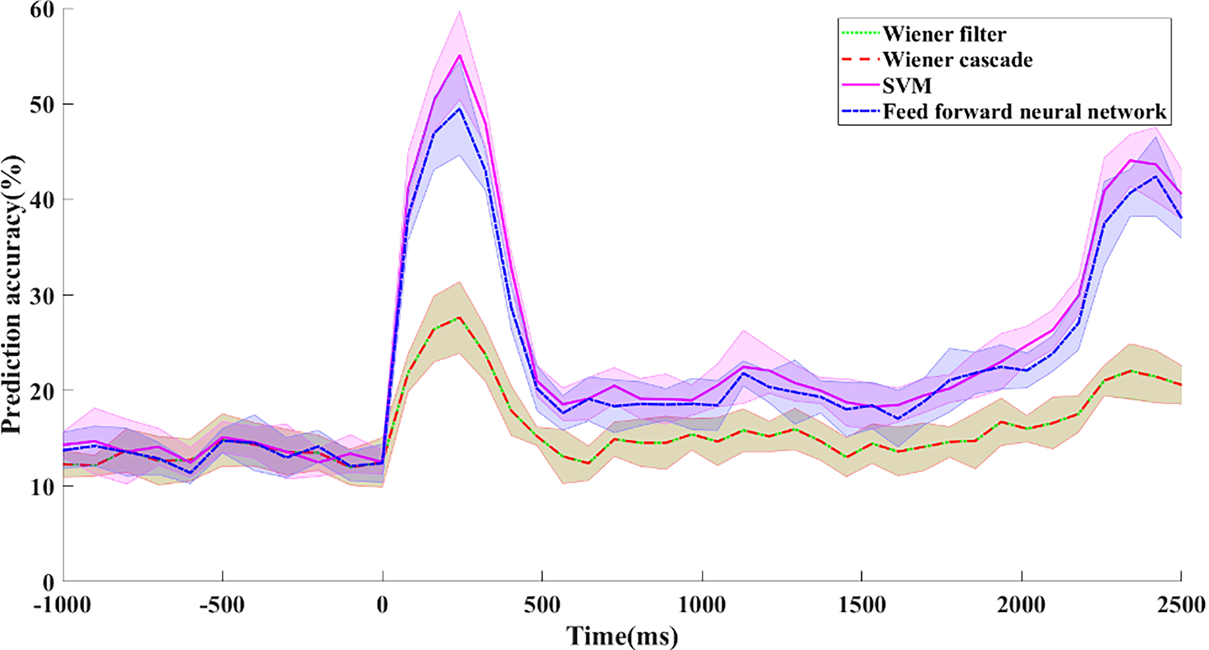

Figure 5.

Prediction accuracy of different SVM kernel functions.

In the next step, vector $x$ is prepared by merging 13 sequential bins with the threshold equal to one and employing 20 successive merged bins. Next, by the provided input space, the aforementioned decoder candidates are trained by 70% of the database and tested by the rest (i.e., 30%). Figure 4 shows the obtained results. In this paper, to present the accuracy of the methods, their performance is evaluated by the prediction accuracy criterion, which is defined as the ratio number of correct answers over the total number of trials.The double-hump line charts are the results of the trial nature. The first hump is caused when the target is shown to the monkey and the second one is related to the saccade time.

As displayed in Fig. 4, the results of the Wiener filter and the Wiener cascade are not accurate enough in comparison with the two others from accuracy aspect, which indicates the relationship between the input model and the output space is too complicated for such simple algorithms to accurately model the actual function. Meanwhile, the results of the feed-forward neural network are related to a network with 400 neurons in one of its hidden layers. Although it would be precisely analyzed in Section 7, it can be generally claimed that based on the dimension of input as well as output space, the volume of the computation for the neural network, especially the number of multipliers and non-linear functions, is considerably higher in comparison to the SVM algorithm with a linear kernel function. As a result, since SVM has achieved the most accurate results with a logical computational complexity, it would be elected as the decoding algorithm. In the next step, it is aimed to choose a perfect SVM algorithm that is accurate and has a hardware-friendly architecture.

5. Tuning the proposed method

5.1 SVM kernel function

In the SVM algorithm, the kernel functions which map the input space to another space influence the algorithm performance. Linear, polynomial, sigmoid, and radial basis functions are some common kernel functions [51]. It is essential to investigate the decoding accuracy of the SVM algorithm by different kernel functions and the proposed input space since different kernel functions can improve decoding accuracy and present different computation complexity. Figure 5 shows the results related to different kernel functions.

As illustrated in Fig. 5, the linear function presents the most accurate prediction. Additionally, it is more hardware-friendly since it is less complicated. Therefore, the linear function is selected as the best SVM kernel to process the input data. The decision function of the SVM algorithm can generally classify between just two classes by its sign. However, the final decision should be made between multi-classes in some cases, especially for our database. This issue is further analyzed in the next section.

Figure 6.

Orientation of the SVM binary decision tree.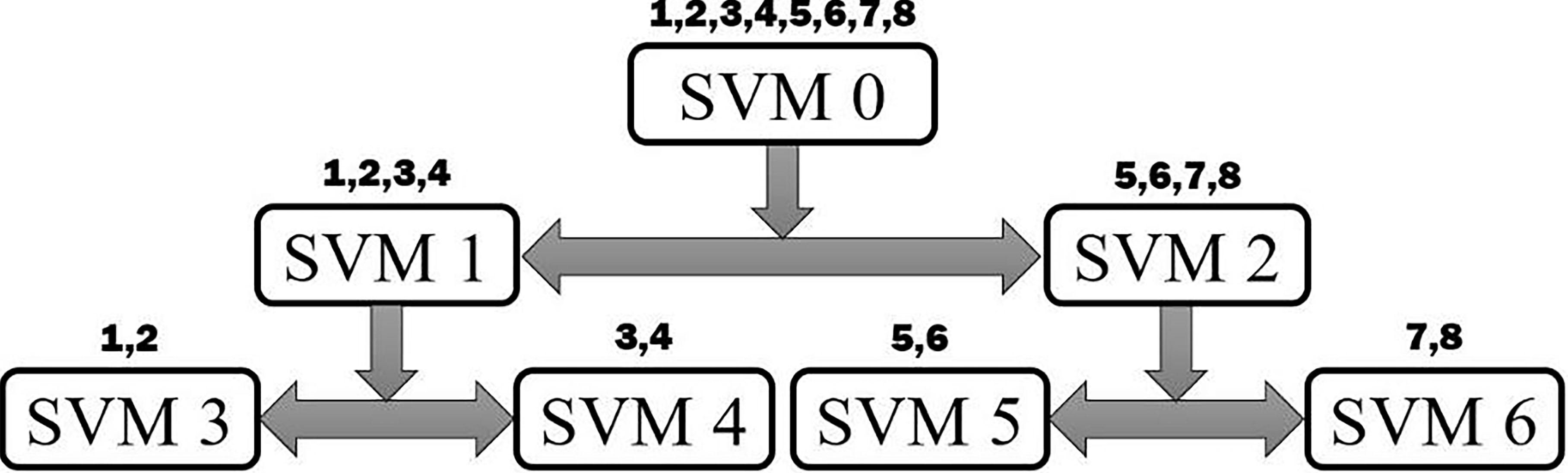

Figure 7.

Prediction accuracy of two different multi-class classifications by binary SVM.

Figure 8.

Flowchart of the proposed decoding algorithm.

5.2 Multi-class classification using binary SVM

Several methods such as binary decision tree [52], one-against-one [53], and one-against-all [54] can be employed to make a multi-class classification with binary classifiers. In the binary decision tree method, all possible classes in the output space are first divided into two subclasses which are repeatedly separated into another two subclasses by another binary SVM in the next steps. On the other hand, in the one-against-one method, there is one specific decision function for each of the two possible classes. After deciding between all possible two classes, the final classification is clarified by the class which has achieved the majority. Finally, in the one-against-all algorithms, one class is classified against all the remaining ones each time. Thus, when a binary SVM is trained for a one-against-all algorithm, the data would be highly unbalanced, especially for a large number of training data, which can reduce the accuracy of the algorithm [55]. Hence, this paper examines only binary decision trees and the one-against-one method.

Eight classes are available as a result of the aforementioned database in Section 2. Therefore, 28 and 7 binary SVMs are required for the one-against-one and binary decision tree method, respectively. Further, although the orientation illustrated in Fig. 6 is utilized for the decision tree, based on several simulations, it is proved that the orientation of the decision tree does not have a significant influence on the accuracy of the method.

In the next step, it is necessary to test both methods under the same condition and evaluate their performance in terms of accuracy and computational complexity. For this reason, Fig. 7 is provided by merging 13 sequential bins with a threshold equal to one and employing 20 successively merged bins as follows:

As mentioned before, the final answer is made by several decision functions and a majority step in one-against-one. More specifically, in this method, even if the signs of some decision functions change, the majority of them still indicate the same class, even in this case the final answer will be correct. On the other hand, even one binary classifier has a critical effect on the final answer in the binary decision tree, and it is more possible for this method to predict a wrong output. Consequently, the one-against-one method is 4.1% more accurate than the other one (Fig. 7).

On the contrary, only 7 SVM is necessary in binary decision tree while this number is 4 times higher for one-against-one, which means more calculations. Based on Fig. 7, although the one-against-one method is 4.1% more accurate, it is neglectable when it is considered with its 4 times more calculation. Accordingly, the binary decision tree method is selected as the multi-class classification algorithm.

Figure 9.

Maximum prediction accuracy versus merging window size.

Figure 10.

Maximum prediction accuracy achieved by several numbers of merged bins.

5.3 Setting algorithm parameters

The structure of the proposed algorithm was determined in previous sections and some parameters should be determined by an offline training process. These items are SVM decision function parameters, merging window size, merged bin number, and the threshold value. The decision function parameters are calculated in the training process while the others should be tuned separately to optimize the accuracy and computational complexity. The flowchart of the proposed method is illustrated in Fig. 8.

The threshold value of the merging step is first considered as one in all tests since the data are based on pre-sorted spikes. Next, as shown in Fig. 8, several window sizes are tested to indicate the merging window size by a reasonable and fixed number of successively merged bins. A graph based on the maximum prediction accuracy per each window size is plotted in Fig. 9. As it is shown, when the window size is too narrow with the constant sequential bins, the total information collected for decoding is too low for accurate results. On the other hand, since the actual number of fires is mapped to zero or one which is actually an approximation, when the window size is too large, the number which is data lost. Therefore, the accuracy decreases dramatically with increasing the window size. The optimum merging size for this database is 9 based on Fig. 9.

After selecting the suitable window size for the merging process, the number of sequential merged bins should be determined. Therefore, similar to the past and flowchart illustrated in Fig. 8, with the previously selected merging window size, the maximum accuracy of the proposed method is plotted with respect to different numbers of sequential bins in Fig. 10.

As shown in Fig. 10, when the number of bins is low, the collected information in the input space is not sufficient for accurate decoding. However, when the number of sequential bins considerably increases, the mapping function between the input and output space would be too complicated for the proposed model to predict the correct answers. Therefore, the optimum number of the sequential merged bins for an accurate result would be 20 based on Fig. 10. In the last stage, all unknown parameters are specified, and the algorithm is ready for online decoding.

Figure 11.

Block diagram of the binary SVM architecture based on the proposed algorithm in this study.

Figure 12.

Block diagram of a multi-channel neural decoder processor based on the proposed decoding approach.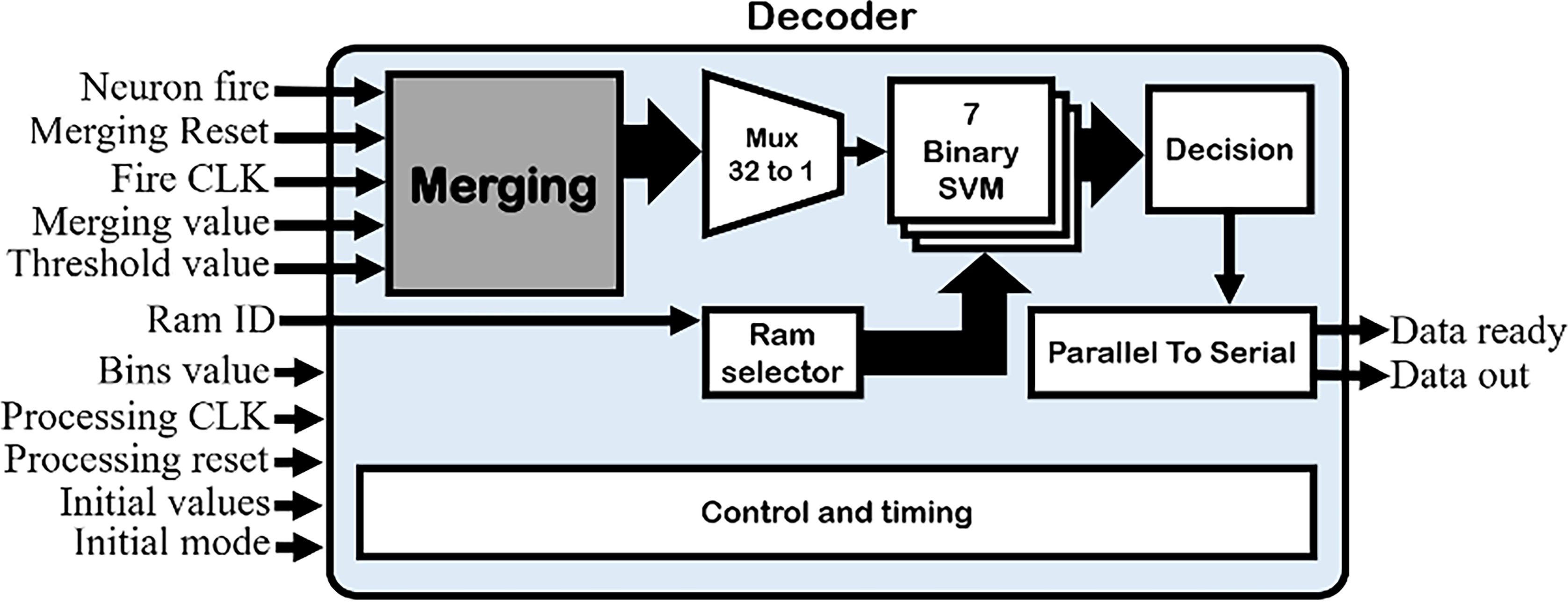

6. Hardware implementation

For implantable BMI applications and hardware implementation, the decoding algorithm should be accurate and as efficient as possible in terms of area and power consumption. Additionally, the system should process the data in real-time as an ideal BMI. Thus, the aforementioned constraints are addressed here. Firstly, an efficient hardware design for one binary SVM module is proposed, which is further utilized in the final structure as a real-time and on-chip decoder.

Since some coefficients and one bias value are necessary for each linear SVM decision function, these parameters should be loaded in the system before any calculation. Figure 11 shows the coefficient and bias RAM modules.

After loading all parameters, the decoder starts its routine calculation. Since all fire inputs are just limited to one or zero, the multiplication operator can be replaced by a multiplexer. Furthermore, to make the design as efficient as possible by utilizing another multiplexer, the output of the accumulator can be directed to its input to continue future calculations or the bias value can be selected as the initial value.

After explaining the binary SVM hardware, the final architecture of the decoder, consisting of 7 binary SVM modules, is proposed (Fig. 12). The final design would have undesirably a considerable number of inputs as a result of 7 binary SVM modules, which should be loaded in the initial step. To eliminate this drawback by utilizing a RAM selector module, just one of the binary SVMs is enabled to accept the related initial values from a common input port.

As illustrated in Fig. 12, the algorithm starts by merging step which should be synchronized with other units. Thus, this unit employs individual clock and resets inputs which are separated from other units by a gray background color. After merging the fires, the merged bin should be utilized for its respect calculations so that each merged fire is directed to a binary SVM module by a 32 to one multiplexer for the aforementioned process.

When all successive bins are received and their decision values are calculated, the final class is determined by the decision unit, which causes outputs by parallel to serial unit to reduce output pins number. Finally, the control and timing unit provides appropriate control and timing signals for all other units.

Figure 13.

The effect of coefficient resolution on the prediction accuracy.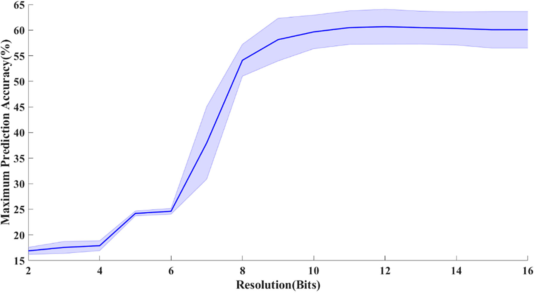

For hardware implementation in addition to the architecture, the resolution of the coefficients and calculation are important. Additionally, the weights and the biases calculated in the training stage should be stored in memory, so their resolution would have a direct effect on the volume of the storage, which is very important in the size of the final chip. Because the boundary of the coefficient is limited, the fixpoint conversion approach is employed on the training step outputs. If the resolution of the coefficients is too low, the accuracy of the decoding algorithm will decline. On the other hand, if the resolution is too high, the computation complexity and its related hardware would be unnecessary too complicated and power hungry in addition to the size. For this reason, the effect of resolution should be investigated by some tests, so in Fig. 13 the maximum gained prediction accuracy chart by resolution is plotted as below:

As it can be observed, when the resolution is too low, the SVM is unable to decode accurately, while by increasing the resolution the decoder performance has improved. The Highest accuracy is achieved around 10 Bits where the results get saturated and higher resolution is almost unaffected anymore. Consequently, the coefficients would be quantized by 10 bits.

Figure 14.

Best achieved prediction accuracy for a) non-recurrent decoders with firing rate inputs b) recurrent neural networks with firing rate inputs and c) the software simulation and hardware implementation results related to the proposed method.

7. Results and discussion

In this section, the performance of the proposed method as well as other commonly used decoding algorithms is evaluated. First, as shown in Fig. 8, the proposed method is tuned to its optimum settings. Since the results of other methods with the employed database are not available, other simulations should be adopted for a reasonable comparison. Therefore, Wiener filter, Wiener cascade, SVM with linear kernel function,and feedforward neural network are selected as non-recurrent methods and LSTM, Elman, and GRU neural networks for the recurrent algorithm analysis. Similar to the proposed routine for the algorithm in this paper, the candidates are set to their optimum parameters by several tests. Therefore, all future results related to the non-recurrent methods are collected by a single-window counting fires with the length of 35 ms and for the recurrent methods in addition to the current firing rate with the same size of non-recurrent ones, 8 windows related to previously calculated firing rates are employed. It should be noted that for other settings, the accuracy of the methods was not as high as the selected ones for this dataset. The simulation results related to non-recurrent methods, which accept firing rate as their input, are illustrated in Fig. 14a.

Table 1
Computational complexity of different decoders

The methods	Non-recurrent			Recurrent		The proposed method	LSTM with the proposed inputs
	Wiener filter	Linear SVM	Feed forward	Elman	LSTM
Add	250	250	16000	176000	695000	4500	695000
Multiply	250	250	16000	176000	695000	0	644000
Non-linear function	0	0	400	400	2000	0	2000
Maximum prediction accuracy	50.4%	42.3%	47.2%	53.9%	61%	62%	62%

Table 2

Amount of FPGA resources usage for the decoders

Methods		JONM 2010 [44]	This paper
		Feed forward neural network	SVM
Resources	Blocks of RAMs	140 Kbytes	5.6 Kbytes
	DSP48E	234	2
	LUT	26,855	1,877
	LUT-FF pairs	10,735	684
	Slice registers	19,423	728

As shown in Fig. 14, almost all non-recurrent methods have similar accuracy although the Wiener filter and SVM have the best and worst results, respectively. Additionally, although both groups of decoders are the same, the results displayed in Figs 4 and 14a are completely different, which is the result of input difference. In Fig. 14, the inputs were the proposed inputs in this paper, while decoders in Fig. 14a utilize firing rates as theirs. The comparison shows that although the SVM method is the same, the more informative input space proposed in this paper improved the accuracy. Figure 14b demonstrates the decoder results related to the recurrent neural networks with firing rate input. The comparison of Fig. 14a and b indicates that recurrent decoders provide more accurate results. They decode based on more information than the non-recurrent ones processing based on just one firing rate, which is due to the fact that they employ several successive firing rates and process their changes over time. Furthermore, between all the cited recurrent algorithms, LSTM yielded the most accurate results and computational complexity between the others. Figure 14c shows the results of the proposed method. Based on the software simulation graph displayed in this figure, although the algorithm is significantly less complicated than with LSTM, the accuracy of its result is almost the same. In addition, the proposed method in this paper is still collectable as a non-recurrent method. However, its accuracy is considerably higher in comparison to the most accurate method in non-recurrent groups, which is due to the special input explained previously.

The complexity of the methods is analyzed (Table 1) which is as important as accuracy for an implantable decoder. To make the analysis as simple as possible, the Wiener filter, linear SVM, and feedforward are selected as the most accurate, least accurate, and a neural network from the non-recurrent decoders, respectively. Additionally, the computational complexity of Elman and LSTM is reported as the least and the most accurate decoders for the recurrent neural networks, respectively. It may be noted that one hidden layer with 400 neurons is used for all types of neural networks.

As shown in Table 1, recurrent methods are generally more complicated but more accurate than non-recurrent ones. LSTM has the most complicated algorithm, and its hardware implementation is very challenging due to its non-linear functions as well as the considerable number of operators. On the contrary, although the accuracy of the proposed method is almost equal to the most accurate method (LSTM), its computational complexity is very low, which is attributed to its simplicity.

As can be observed, as a result of its linearity, no non-linear function is required and as a result of its inputs which are just one and zero, it does not use the multiplier.

As shown in Table 1, the input space proposed in this paper increases SVM accuracy; moreover, LSTM is a very accurate algorithm. Therefore, it would be interesting to analyze the performance of the same LSTM algorithm but with the proposed input space. Hence, in Table 1 the result of the cited simulation is collected in another column. The results indicate that not only the input has not improved the accuracy anymore, but also the computational complexity of the algorithm is very high. Therefore, the SVM is the best method for the input space, especially when the accuracy is considered with its computational complexity.

Generally, when an algorithm is replicated as a hardware, the system loses some of its accuracy due to quantization errors. Thus, it is necessary to test this effect on the proposed method. The results of the designed hardware as well as those related to the simulation are shown in Fig. 14c. Comparison of the two graphs shows that the hardware design has lost some of its accuracy although it is still very accurate, which is caused by the decision section of the algorithm which is just based on the signs of the calculated values. Therefore, the final result would be the same as long as the error of the quantization does not change the sign of the actual number. Hence, the algorithm is accurate as a hardware design and is robust to quantization error.

Finally, the performance of the proposed method should be evaluated in terms of area and power aspects. Since the algorithms are implemented based on field-programmable gate array (FPGA) in some methods and based on the application-specific integrated circuit (ASIC) in some others, in this paper both comparisons are reported. Therefore, the proposed method is firstly developed under Xilinx ISE 14.7 for Xilinx Virtex5 vsx50 FPGA and the synthesized report is presented in Table 2 as below beside the other method employing similar FPGA.

Since the proposed method is based on seven linear binary SVMs and as a result of the input space, the simple method does not require any multiplication and the usage resources of the FPGA are much less than a non-recurrent neural network decoder such as the one presented in [44]. Additionally, although the proposed method in this paper employed many coefficients which are stored in RAMs, the occupied RAMs are still less than the necessary volume for the neural network implementation, which has a more complicated structure with a lot of coefficients.

From power consumption and area aspects FPGA implementation is not suitable for an implantable BMI although it covers some of the BMI essentials such as real-time processing. Therefore, the ASIC approach is adopted. The obtained results from post-layout simulation are listed in Table 3. As can be seen in Table 3, the calculations in both methods are performed by the SVM algorithm and the technology and its supply voltage for the proposed method are more than the other one. However, the ASIC design in this paper is smaller and has less power dissipation, which is mostly due to the proposed input space.

Table 3

Results related to ASIC design for the decoders

Methods	JSSC 2013 [56]	This paper
	SVM	SVM
Technology	130 nm	180 nm
Supply voltage	0.85 v	1.8 v
Application	EEG analysis	Neural implant
Chip size	5.13 mm ${}^{2}$	4.15 mm ${}^{2}$
Power dissipation	136.5 $\mu$ w	28.58 $\mu$ w
Resolution	16 bits	10 bits
Classification rate	0.5–2 Hz	5.56 Hz

8. Conclusion

In this study, a new input space as well as a modified SVM algorithm was proposed as a hardware-friendly, low power, area efficient, and online neural decoding approach. The most important finding of this study was that the new inputs which could simplify the computational complexity and improve accuracy of the outputs as a result of more informative features and limitation to just one and zero. The evaluations showed that the accuracy of the suggested method was generally higher than the non-recurrent method and almost equal to recurrent methods, especially LSTM. This fact was noticeable when the computational complexity of the proposed method was compared with the recurrent methods. Finally, since hardware implementation was one of the main constraints of this study, the proposed hardware architecture was compared with FPGA and ASIC-based implementation. In both platforms, it was determined that the system utilized fewer resources and the architecture had far more acceptable results in terms of area and power for the ASIC design.

It can be noted from the presented results, in the past when it was desired to improve the accuracy of a method such as Wiener filter to be a very accurate decoder like LSTM, the volume of necessary hardware resources should be noticeably increased, while by the proposed method in this paper the incremented resources are more logical with considering the improved accuracy. Therefore, the proposed method is accurate and hardware-friendly decoder. On the other hand, Although the proposed method has improved the decoding accuracy equal to a very accurate algorithm such as LSTM but with logical computational complexity, the system accuracy improvement is not still equal to its inclement in computational complexity when it is compared with very simple decoders (for example wiener filter). In this reason, it can be suggested the proposed algorithm is just suitable for applications when high accuracy is required and some more computational complexity is acceptable simultaneously, especially when too complicated approaches such as recurrent methods is not possible.

Finally, it was shown that considering temporal information can improve the accuracy of decoding process, which can be achieved by adding spatial information to the algorithm and processing the data as a 2D image even more. This will help to improve the performance without accepting too much computational complexity.

Footnotes

Acknowledgments

The authors would like to thank Behrad Noudoost for sharing the experimental data which served as the basis for evaluation in this study.

References

Liu

Zhang

Richardson

Lucas

Van der Spiegel

. Design of a Closed-Loop, Bidirectional Brain Machine Interface System With Energy Efficient Neural Feature Extraction and PID Control. IEEE Trans Biomed Circuits Syst. 2016; 11(4): 729-742.

Burns

Adeli

. Wearable technology for patients with brain and spinal cord injuries. Reviews in the Neurosciences. 2017 Dec 1; 28(8): 913-920.

Chaudhary

Chander

Ohry

Jaramillo-Gonzalez

Lule

Birbaumer

. Brain Computer Interfaces for Assisted Communication in Paralysis and Quality of Life. International Journal of Neural Systems. 2021 Sep 29; 31(11).

Ortiz-Rosario

Adeli

. Brain-computer interface technologies: from signal to action. Reviews in the Neurosciences. 2013 Oct 1; 24(5): 537-552.

Brandman

Cash

Hochberg

. Review: Human Intracortical Recording and Neural Decoding for Brain – Computer Interfaces. IEEE Transactions on Neural Systems and Rehabilitation Engineering. 2017; 25(10): 1687-1696.

Yao

Wang

Yang

Pei

Gao

Chen

. An online brain-computer interface in mobile virtual reality environments. Integrated Computer-Aided Engineering. 2019; 26(4): 345-360.

Ahmadi-Dastgerdi

Hosseini-Nejad

Amiri

Shoeibi

Gorriz

. A Vector Quantization-Based Spike Compression Approach Dedicated to Multichannel Neural Recording Microsystems. International Journal of Neural Systems. 2021. DOI: 10.1142/S0129065722500010.

Vidal

. Toward direct brain-computer communication. Annual Review of Biophysics and Bioengineering. 1973; 2(1): 157-180.

Burns

Adeli

Buford,

. Upper Limb Movement Classification Via Electromyographic Signals and an Enhanced Probabilistic Network. J Med Syst. 2020; 44(10).

10.

Rafiei

Kelly

Borstad

Adeli

Gauthier

. Predicting improved daily use of the more affected arm poststroke following constraint-induced movement therapy. Physical Therapy. 2019 Dec 16; 99(12): 1667-1678.

11.

Buzsáki

Anastassiou

Koch

. The origin of extracellular fields and currents-EEG, Eco, LFP and spikes. Nat Rev Neurosis. 2012; 13(6): 407-420.

12.

Hochberg

Serruya

Friehs

Mukand

Saleh

Caplan

Branner

Chen

Penn

Donoghue

. Neuronal ensemble control of prosthetic devices by a human with tetraplegia. Nature. 2006 Jul; 442(7099): 164-171.

13.

Kim

Simeral

Hochberg

Donoghue

Black

. Neural control of computer cursor velocity by decoding motor cortical spiking activity in humans with tetraplegia. J Neural Eng. 2008 Dec; 5(4): 455-476.

14.

Simeral

Kim

Black

Donoghue

Hochberg

. Neural control of cursor trajectory and click by a human with tetraplegia 1000 days after implant of an intracortical microelectrode array. J. Neural Eng. 2011 Apr; 8(2): 25027.

15.

Jarosiewicz

Sarma

Bacher

Masse

Simeral

Sorice

Oakley

Blabe

Pandarinath

Gilja

Cash

. Virtual typing by people with tetraplegia using a self-calibrating intracortical brain-computer interface. Sci Transl Med. 2015; 7(313): 1-11.

16.

Hochberg

Bacher

Jarosiewicz

Masse

Simeral

Vogel

Haddadin

Liu

Cash

Van Der Smagt

Donoghue

. Reach and grasp by people with tetraplegia using a neurally controlled robotic arm. Nature. 2012 May; 485(7398): 372-375.

17.

Wodlinger

Downey

Tyler-Kabara

Schwartz

Boninger

Collinger

. Ten-dimensional anthropomorphic arm control in a human brain-machine interface: difficulties, solutions, and limitations. J. Neural Eng. 2015; 12(1): 16011.

18.

Monk

Leib

. A Model for Single Neuron Activity With Refractory Effects and Spike Rate Estimation Techniques. IEEE Transactions on Neural Systems and Rehabilitation Engineering. 2017; 25(4): 306-322.

19.

Dayan

Abbott

. Theoretical Neuroscience: Computational and Mathematical Modeling of Neural Systems. Massachusetts Institute of Technology Press. 2001.

20.

Rieke

Warland

Van Steveninck

Bialek

. Spikes: Exploring the Neural Code. A Bradford Book. 1999.

21.

Feng

Zeng

. Neural Decoding for Macaque’s Finger Position: Convolutional Space Model. IEEE Trans Neural System and Rehabilitation Engineering. 2019; 27(3): 543-551.

22.

Lewicki

. A review of methods for spike sorting: The detection and classification of neural action potentials. Network Computation in Neural Systems. 1998; 9(4): R53-R78.

23.

Pohlmeyer

Solla

Perreault

Miller

. Prediction of upper limb muscle activity from motor cortical discharge during reaching. Neural Eng. 2007; 4(4): 369-379.

24.

Dehaqani

Vahabie

Parsa

Noudoost

Soltani

. Selective Changes in Noise Correlations Contribute to an Enhanced Representation of Saccadic Targets in Prefrontal Neuronal Ensembles. Cereb Cortex. 2018; 28(8): 3046-3063.

25.

Zhang

Wang

Cui

. Generative Decoding of Intracortical Neuronal Signals for Online Control of Robotic Arm to Intercept Moving Objects, in Journal of Physics: Conference Series, Volume 1576, 4th International Conference on Artificial Intelligence, Automation and Control Technologies (AIACT 2020). Hangzhou, China, 2020.

26.

Pereira

Piteri

Souza

Papa

Adeli

. FEMa: A finite element machine for fast learning. Neural Computing and Applications. 2020 May; 32(10): 6393-6404.

27.

Rafiei

Adeli

. A new neural dynamic classification algorithm. IEEE Transactions on Neural Networks and Learning Systems. 2017 Jul 25; 28(12): 3074-3083.

28.

Baggenstoss

. On the Duality Between Belief Networks and Feed-Forward Neural Networks. IEEE Transactions on Neural Networks and Learning Systems. 2019; 30(1): 190-200.

29.

Alam

Siddique

Adeli

. A dynamic ensemble learning algorithm for neural networks. Neural Computing and Applications. 2020 Jun; 32(12): 8675-8690.

30.

George

Rafiei

Borstad

Adeli

Gauthier

. Gross motor ability predicts response to upper extremity rehabilitation in chronic stroke. Behavioural Brain Research. 2017 Aug 30; 333: 314-322.

31.

George

Rafiei

Gauthier

Borstad

Buford

Adeli

. Computer-aided prediction of extent of motor recovery following constraint-induced movement therapy in chronic stroke. Behavioural Brain Research. 2017 Jun 30; 329: 191-199.

32.

Rosenblatt

. Principles of Neurodynamics. Spartan Books. 1962.

33.

Glaser

J. I.

Benjamin

A. S.

Chowdhury

R. H.

Perich

M. G.

Miller

L. E.

and Kording

K. P.

Machine learning for neural decoding. Neurons and Cognition. 2017.

34.

Ergen

Kozat

. Online Training of LSTM Networks in Distributed Systems for Variable Length Data Sequences. IEEE Transactions on Neural Networks and Learning Systems. 2018; 29(10): 5159-5165.

35.

Heelan

Nurmikko

Truccolo

. FPGA implementation of deep-learning recurrent neural networks with sub-millisecond real-time latency for BCI-decoding of large-scale neural sensors (104 nodes). 2018 40th Annual International Conference of the IEEE Engineering in Medicine and Biology Society (EMBC). Honolulu, HI, USA. 2018.

36.

Sun

Tian

Zhang

Wang

. Design of blender IMC control system based on simple recurrent networks. 2009 International Conference on Machine Learning and Cybernetics. Hebei, China. 2009.

37.

Heck

Salem

. Simplified minimal gated unit variations for recurrent neural networks. IEEE 60th International Midwest Symposium on Circuits and Systems. 2017.

38.

Aghagolzadeh

Truccolo

. Latent state-space models for neural decoding. Proc. IEEE 36th Annu Int Conf Eng Med Biol Soc Chicago, IL, USA. 2014 Aug: 3033-3036.

39.

Aghagolzadeh

Truccolo

. Inference and Decoding of Motor Cortex Low-Dimensional Dynamics via Latent State-Space Models. IEEE Transactions on Neural Systems and Rehabilitation Engineering. 2016; 24(2): 272-282.

40.

Song

Hsieh

Shanechi

. Decoder for Switching State-Space Models with Spike-Field Observations. 9th International IEEE/EMBS Conference on Neural Engineering (NER). San Francisco, CA, USA, USA. 2019.

41.

Chew

Ang

Guan

. Combining Firing Rate and Spike-Train Synchrony Features in the Decoding of Motor Cortical Activity. Proc IEEE Eng Med Biol Soc. 2015.

42.

Satuvuori

Kreuz

. Which spike train distance is most suitable for distinguishing rate and temporal coding? Journal of Neuroscience Methods. 2018; 299: 22-33.

43.

Chen

Yao

Basu

. A 128-Channel Extreme Learning Machine-Based Neural Decoder for Brain Machine Interfaces. IEEE Trans Biomed Circuits Syst. 2015; 10(3): 679-692.

44.

Zhou

Liu

Tian

Liu

Hao

Zhang

Chen

Dai

Zheng

. Field-programmable gate array implementation of a probabilistic neural network for motor cortical decoding in rats. Journal of Neuroscience Methods. 2010; 185(2): 299-306.

45.

Kreuz

Chicharro

Houghton

Andrzejak

Mormann

. Monitoring spike train synchrony. J. Neurophysiol. 2013; 109: 1457-1472.

46.

Decharms

Zador

. Neural representation and the cortical code. Annual Review of Neuroscience. 2000; 23: 613-647.

47.

Bair

Koch

. Temporal precision of spike trains in extrastriate cortex of the behaving macaque monkey. Neural Computation. 1996; 8(6): 1185-1202.

48.

Buracas

Zador

DeWeese

Albright

. Efficient discrimination of temporal patterns by motion-sensitive neurons in primate visual cortex. Neuron. 1998; 20(5): 959-969.

49.

Salinas

Sejnowski

. Correlated neuronal activity and the flow of neural information. Nature Review Neurosci. 2001; 2(8): 539-550.

50.

Ran

Zhang

Sun

Zhu

Chen

Pan

. Decoding Velocity from Spikes Using a New Architecture of Recurrent Neural Network. 9th International IEEE/EMBS Conference on Neural Engineering (NER). San Francisco, CA, USA. 2019.

51.

Chang

Lin

. LIBSVM: a library for support vector machines. ACM Transactions on Intelligent Systems and Technology. 2011; 2(3).

52.

Madzarov

Gjorgjevikj

Chorbev

. A Multi-class SVM Classifier Utilizing Binary Decision Tree. Informatica (Slovenia). 2009; 33(2): 225-233.

53.

Gustian

Rohmah

Shidik

Fanani

Pramunendar

. Classification of Troso Fabric Using SVM-RBF Multi-class Method with GLCM and PCA Feature Extraction. 2019 International Seminar on Application for Technology of Information and Communication (iSemantic). Semarang, Indonesia, Indonesia. 2019.

54.

Liu

Hao

Yang

. Modifying the Decision Function in One-Against-All Algorithm for Multi-Classification. 2006 International Conference on Machine Learning and Cybernetics. Dalian, China, China. 2006.

55.

Wang

Zhang

and Zhou

. A total error rate multi-class classification. 2012 IEEE International Conference on Systems, Man, and Cybernetics (SMC). Seoul, South Korea. 2012.

56.

Lee

Verma

. A low-power processor with configurable embedded machine-learning accelerators for high-order and adaptive analysis of medical-sensor signals. IEEE J. Solid-State Circuits. 2013 Jul; 48(7): 1625-1637.

A hardware efficient intra-cortical neural decoding approach based on spike train temporal information

Abstract

Keywords

1. Introduction

3. Inputs model

5.1 SVM kernel function

Table 1 Computational complexity of different decoders

Footnotes

Acknowledgments

References

Table 1
Computational complexity of different decoders