Heat Map Based Feature Ranker: In depth comparison with popular methods

Abstract

The new era of technology allows us to gather more data than ever before, complex data emerge and a lot of noise can be found among high dimensional datasets. In order to discard useless features and help build more generalized models, feature selection seeks a reduced subset of features that improve the performance of the learning algorithm. The evaluation of features and their interactions are an expensive process, hence the need for heuristics. In this work, we present Heat Map Based Feature Ranker, an algorithm to estimate feature importance purely based on its interaction with other variables. A compression mechanism reduces evaluation space up to 66% without compromising efficacy. Our experiments show that our proposal is very competitive against popular algorithms, producing stable results across different types of data. We also show how noise reduction through feature selection aids data visualization using emergent self-organizing maps.

Keywords

Feature selection high-dimensional data self-organizing maps

1. Introduction

In the past decade, thanks to numerous improvements in technology it is possible to capture more data than ever before, hence, increasing the dimensionality for several machine learning applications [8]. Notable areas with a very high increase in data dimensionality are Bio-informatics and microarray analysis [35], where several thousand of features per sample are common nowadays. However, these high-dimensional datasets usually are plagued with irrelevant and noisy features, therefore generalization performance can be improved by using only good features [28] while also getting additional benefits in the form of reduced computational cost.

The increase in dimension (features) leads to a phenomenon called the curse of dimensionality where data becomes sparse in a high dimensional space which causes issues with algorithms not designed to handle such complex spaces [16]. To mitigate this problem it is imperative to do some dimensionality reduction. Since 1960 this has been under research community investigation [18], it had an important boom in 1997 with special issues on its relevance [4, 21], however back then only a very minimal set of domains had more than 40 features [15].

In order to achieve the goal of dimensionality reduction, there are two main approaches, feature extraction and feature selection. The feature extraction approach seeks to transform the high dimensional features into a whole new space of lower dimensionality, usually, by a linear or nonlinear combination of the original set of features, an example of these techniques are Principal Component Analysis (PCA) [37] and Singular Value Decomposition (SVD) [12].

In this paper, we will focus on the other approach which is feature selection, as this is usually a more useful method in a real life scenario where it is important to understand which features of the original space are the most representative. Nonetheless, both approaches aim to have a reduced number of features [7] as experimentation has shown that a subset of features may help reduce overfitting [19].

Since 1980 we can see the development of several algorithms for feature selection that have been successful in different areas such as: Text categorization [11], pattern recognition [26], image processing [32] and bioinformatics [33]. However, more than three decades of research have not yet found an all-around best algorithm and many conclusions lead to believe that the solution is data-dependent. Therefore it is very important to continue the development of new approaches to handle different scenarios in the data, however, even with considerable options in algorithms, the key idea remains the same; try to keep the most relevant features and remove the rest.

There are several proposals to define what a relevant feature is, however in this paper we take the definition of John et al. [20] where they establish two different kinds of relevance:

•
Strong relevance: are features that, if removed, would cause a drop in classifier performance.
•
Weak relevance: these features can be removed from the full set without considerably affecting the classifier performance.

Any feature that is not relevant is therefore irrelevant and could be divided into two main groups:

•
Redundant features: those that do not provide any new information about the class and therefore can be substituted by another feature.
•
Noisy features: includes the features that are not redundant but, do not provide useful information about the class either.

In the seek for these relevant features, there are at least 4 key parameters that affect the search performance [4]:

•
Search direction:

–
Forward: we start with an empty set of features and new ones are being added once they are evaluated as useful.
–
Backward: the full set of features are setup at first and then irrelevant features are being dropped.

•
Search strategy: These are based on corresponding heuristics for each algorithm, one example could be Greedy search.
•
Evaluation criterion: how the features are selected, the criteria or threshold that needs to be overcome in order to tag a feature as useful.
•
Stopping criterion: this determines if the algorithm will just stop after a given number of iterations or will hold until a given threshold could be reached, this has a direct impact on the feature set size, where the optimal size may be defined by the number of instances [27].

When designing a feature selection algorithm there are at least three challenges to address [2]:

•
Small sample size: as the number of features increases, the number of instances required to produce a stable selection increase as well, however, there are many areas where samples are expensive to gather and the result is a dataset with thousands of features with only hundreds of samples which makes the process prone to overfitting.
•
Data noise: if the algorithm is not robust enough, noisy features would guide the selection erroneously as the algorithm will try to learn the noise as if it were a real pattern.
•
Selected features: algorithms that only rank features have to deal with the issue of how many features to choose for the final subset. Some other approaches use thresholds to automatically select the number of features.

Supervised feature selection algorithms use the statistical relation between the data and the labels [15] to select the features. These algorithms can be divided into three major groups: Filter, Wrapper, and Hybrid [2]. For low-dimensional data, it is possible to use different techniques, even the wrapper approach could be used, but once the dimension grows at a considerable scale of thousand of features, the computation complexity becomes a problem, and the filter approach, being the more efficient becomes a very popular option. Our algorithm is a filter approach.

•
Filter model: these algorithms are completely independent of any classifier, hence the final selection depends only on the characteristics of the data itself and its relation to the target [13, 38]. Filter models are overall very efficient, scalable and their results are usually portable as they do not depend on external components such a guiding classifier, these advantages make them very suitable for high dimensional data.
•
Wrapper model: these algorithms use a classifier to evaluate their performance [20, 21], the initial feature selection is usually achieved by a greedy search strategy, the classifier performance is evaluated with the selected features and if the result is satisfactory the search stops, otherwise the whole process is repeated again but this time with a different subset. This is a very expensive process usually applied for low-dimensional data only.
•
Hybrid model: As we have seen the filter models are more efficient, while the wrapper models are usually more accurate, in order to achieve a balance, the hybrid model is proposed to fill the gap between those approaches [6]. In the search step they employ a filter selection to reduce the number of candidates, later a classifier is used to select the subset that provided the best accuracy.

For low-dimensional data, it is possible to use different techniques, even the wrapper approach could be used, but once the dimension grows at a considerable scale as thousand of features, the computation complexity becomes a problem and the filter approach being the more efficient becomes most of the time the only feasible option.

In a previous work [17] we compared our algorithm Heat Map Based Feature Selection (HmbFS) with three well-known feature selection techniques, this work presents a ranking variation of the original HmbFS algorithm, a more in depth comparison, new datasets and algorithms to provide a better understanding of its capabilities.

The remaining of this paper is structured as follows: In Section 2, related work is being presented. In Section 3 we present HmbFS formal definition and discuss how it works. In Section 4 we describe our experiments and results. In Section 5 we present the final conclusions and discuss future work.
2. Related work

There are multiple techniques used for feature selection, according to the work of Li et al. [22], we can identify some groups of algorithms based on their fundamental idea, in this work we consider: information theoretical (MRMR, CIFE, CMIM, DISR), similarity based (ReliefF, Fisher) and statistical based (Gini). Although the main idea behind every algorithm remains the same, each of them presents their unique formulation for feature importances, in the following paragraphs we give a brief introduction for each algorithm.

2.1 Fisher score

This algorithm performs selection based on the difference of feature values, under the rationale that samples within same class have small differences and features values from other classes are larger [9]. The usefulness of each feature is calculated as follows:

$\displaystyle F_{\textit{score}}(f_{i})=\frac{\sum\limits_{j=1}^{c}n_{j}(\mu_{% i,j}-\mu_{i})^{2}}{\sum\limits_{j=1}^{c}n_{j}\sigma_{i,j}^{2}}$ (1)

As it can be seen from Eq. (1), the feature score is calculated from the difference between the mean for each feature $(\mu_{i})$ and the feature mean for a particular class $J(\mu_{i,j})$ . Also considering the feature variance $(\sigma)$ to penalize noisy features.

2.2 ReliefF

The Relief algorithm was originally designed to solve binary problems only, however, the ReliefF variant provides an extension to tackle multi class data [31]. The feature score is calculated as follows:

$\displaystyle Z=d(X(j,i)-X(r,i))$ (2) $\displaystyle\textit{relief }F_{\textit{score}}(F)=\frac{1}{c}\sum\limits_{j=1% }^{l}\left(-\frac{1}{m_{j}}\sum\limits_{x_{r}\in NH(j)}Z+\sum\limits_{y\neq y_% {j}}\frac{1}{h_{jy}}\frac{p(y)}{1-p(y)}\sum\limits_{x_{r}\in NM(j,y)}Z\right)$ (3)

Where $\textit{NH}(j)$ stands for near-hit and $\textit{NM}(j,y)$ near-miss, which makes reference to the nearest instance to $x_{r}$ with the same (hit) class label and different (miss) class respectively. The main idea is to take a random subsample of instances $l$ of size $h_{jy}$ and $m_{j}$ for near-hits and near-miss respectively and calculate the distance between them as in Eq. (2) usually by the Euclidean distance. The ratio $p(y)$ of instances belonging to a class $y$ is also considered for evaluation.

2.3 MRMR

The minimum redundancy and maximum relevance (MRMR) [29] algorithm is based on mutual information feature selection (MIFS) [3] and it is calculated as follows:

$\displaystyle\textit{MRMR}(X_{k})=I(X_{k};Y)-\frac{1}{\mid S\mid}\sum_{X_{j}% \in S}I(X_{k};X_{j})$ (4)

First part of Eq. (4) gives us the feature importance given its information gain and the second term is used to penalize feature redundancy with the already selected features $S$ . A key difference with other techniques is that the parameter $\beta$ is replaced for the inverse of the selected features $\frac{1}{\mid S\mid}$ instead of 1 as in MIFS.

2.4 CIFE

The Conditional Infomax Feature Extraction (CIFE) algorithm [23] presents the idea of conditional redundancy as other studies [1] have shown that the redundancy evaluation performed by MRMR or MIFS could be improved. The resultant equation now includes a third term as shown below:

$\displaystyle\textit{CIFE}(X_{k})=I(X_{k};Y)-\sum_{X_{j}\in S}I(X_{j};X_{k})+% \sum_{X_{j}\in S}I(X_{j};X_{k}\mid Y)$ (5)

2.5 CMIM

As shown by Brown et al. [5], information theoretic based algorithms can be reduced to a linear combination of Shannon information terms, one example is Conditional Mutual Information Maximization (CMIM) [10], where the main idea is to add features that maximize the mutual information with the target but those features need to look different to already selected ones, even if they have strong predictive power. The equation is as follows:

$\displaystyle\textit{CMIM}(X_{k})=I(X_{k};Y)-\max_{X_{j}\in S}[I(X_{j};X_{k})-% I(X_{j};X_{k}\mid Y)]$ (6)

2.6 DISR

Another technique is Double Input Symmetrical Relevance (DISR) [25] which uses normalization techniques, hence it normalizes mutual information as follows:

$\displaystyle\textit{DISR}(X_{k})=\sum_{X_{j}\in S}\frac{I(X_{j}X_{k};Y)}{H(X_% {j}X_{k}Y)}$ (7)

As with other techniques, DISR can also be reduced to a conditional likelihood maximization framework.

2.7 Gini index

The idea behind Gini index is to identify which features are able to separate instances from different classes given if features values are lower or greater than a reference point. The equation is as follows:

$\displaystyle\textit{Gini}(f_{i})=\min_{W}\left(p(W)\left(1-\sum_{s=1}^{C}p(C_% {s}\mid W)^{2}\right)+p(\overline{W})\left(1-\sum_{s=1}^{C}p(C_{s}\mid% \overline{W})^{2}\right)\right)$ (8)

Unlike other algorithms, in the case of Gini index, the idea is to minimize the score. In Eq. (8), $C_{s}$ makes reference to class label being $s$ , and $W$ & $\overline{W}$ are the set of instances with feature value below and above to the reference split.

Every algorithm has its pro and cons due to their specific designs, given their mathematical formulations, it is hard to estimate their performance in real life situations. Hence, in this work, we perform a practical evaluation using real-world datasets with complex features-to-samples ratios.

3. Heat map based ranker

A core part of our algorithm is working with heat maps, which is commonly used in high dimensional spaces such as genomic data to unravel hidden patterns, in recent studies we can see how heatmaps are being used to understand data structure [14] so for this work we use an internal heatmap generation to aid in the search of regions of interest.

The idea behind Heat Map Based Feature Ranker (HmbFR) is to estimate the predictive power of a feature given its association with others, an exhaustive feature combination is avoided under the rationale that high dimensional data usually keeps an intrinsic structure. Even if this order does not apply to all datasets, we consider the evaluation of features in groups of continuous features as a useful approach for high dimensional data.

The algorithm is composed of two main stages: compression and ranking. The core idea is to build groups of features and later evaluate their predictive power as a group to estimate individual feature power.

In compression stage, we build the heat map, which is a color representation of the data, in order to build it, a color model is required, since our design uses groups of 3 features, the RGB model is a perfect fit as it requires three channels, therefore 3 features $F$ are used to build 1 group $G$ of the form $G_{i}=\{F_{r},F_{g},F_{b}\}$ , these elements stand for $\textit{Feature}_{\textit{Red}}$ , $\textit{Feature}_{\textit{Green}}$ and $\textit{Feature}_{\textit{Blue}}$ and the relation between a particular group of features creates a pattern, such pattern is mapped to a color in a virtual heatmap, and this color is what is further analyzed in order to decide if the group of features should be kept. These groups are built by continuous features, in two stages, forward and backwards, so in the original space $F_{1}$ , $F_{2}$ and $F_{3}$ becomes $G_{1}$ for the forward stage and, for $N$ features, the backward stage $G_{1}$ is represented by $F_{n}$ , $F_{n-1}$ and $F_{n-2}$ .

The first step for compression is the normalization isolated features, each of them is treated independently, to formalize this, let $I$ be the full set of instances and $I_{x}$ a particular sample from the whole dataset $D$ . Each value $F_{i}$ that belongs to instance $I_{x}$ ( $I_{x}F_{i}$ ) is then normalized in a 0 to 255 interval as shown in Eq. (3):

$\displaystyle\quad\quad\quad\forall I_{x}F_{i}\in D:$ $\displaystyle\widehat{I_{x}F_{i}}=\left(\frac{I_{x}F_{i}-\text{min}(FI_{x})}{% \text{max}(FI_{x})-\text{min}(FI_{x})}\right)*255$ (9)

Where $\min(IF_{i})$ and $\max(IF_{i})$ represents the minimum and maximum value respectively that a feature gets across all the instances of the dataset. This process is repeated for every feature $F_{i}$ across all instances $I_{x}$ . Once the features have been normalized, each of the groups containing $F_{r}$ , $F_{g}$ and $F_{b}$ can be mapped to a true color expressed in red/green/blue (RGB) format, together the three features can represent up to 16,777,216 different colors or patterns. However, since the idea is to build a generalization of the original data, we apply a technique called Color Quantization that allows the mapping of a true color to a lower depth color scale, in this case, we reduce each true color to a 4-Bit 16-Colors scheme. The idea is to discard small data variations or uniqueness, and produce a new set of data which is more general and consistent, the process of quantization is performed by looping over the 16 reference colors and find the minimum Euclidean distance with the true color as this approach is very popular for the task and it has been found to produce satisfactory results [30]. The RGB values for each of those colors are the standard values defined in the HTML 4.01 specification.1

https://www.w3.org/TR/html4/types.html#h-6.5.

To formalize the information quantization, let $G$ be the set of all the built groups and $G_{i}$ a particular group (which is composed by $F_{r}$ , $F_{g}$ and $F_{b}$ ) that belongs to a instance $I_{x}$ , each of those $I_{x}G_{i}$ combinations are then compared against all the reference colors $R_{j}$ in set $R$ to produce the new single-value compressed feature $F_{i}$ that will represent the original 3-feature as shown below:

$\displaystyle\forall I_{x}G_{i}\in D\textit{ and }\forall j\in\{1,...,16\}:$ $\displaystyle I_{x}F_{i}=\min\left(\sqrt{\begin{aligned} \displaystyle(I_{x}G_% {i}F_{r}-R_{j}F_{r})^{2}+\\ \displaystyle(I_{x}G_{i}F_{g}-R_{j}F_{g})^{2}+\\ \displaystyle(I_{x}G_{i}F_{b}-R_{j}F_{b})^{2}\end{aligned}}\right)$ (10)

Once all the distances between true color and reference color have been calculated, we select the reference color $R_{j}$ with the minimum Euclidean distance, and this process gives origin to a new dataset that is purely built in reference colors, or in other words, it is a compressed lossy version of the original.

Dataset reduction is possible due to the fact that the reference color is represented by a single value (e.g. red, which is composed of RGB values of 255,0,0) instead of three different features, this compression makes possible to reduce the original dimension of any dataset to a third with very minimal loss of information, however although there is indeed a loss, this can be negligible as the data transformation is only used for the feature selection process, and the original information suffers no changes.

After compression is completed, ranking relevant features is based on the rationale that different classes should look different, hence their associated quantized colors should look different as well. The ranking occurs in the new compressed dataset, the process sees regular features $F_{i}$ although we know they represent a group in the original space.

[b]

Dataset with full number of features Subset of best predictive features Normalize Data 0–255;

there are more features \\Compression $F_{i}$ , $F_{i+1}$ , and $F_{i+2}$ Build group $G_{i}$ with features as 16-Bit RGB values;

Save quantized 4-bit version of $G_{i}\rightarrow QG_{i}$ ; Increase $i$ by 3; each group $QG_{x}$ \\Ranking each class $K_{i}$ each class $K_{j}$ != $K_{i}$ each color $C_{r}$ $QG_{x}=QG_{x}+\Big{(}Pr(C_{r}\mid K_{i})-Pr(C_{r}\mid K_{j})\Big{)}$

HmbFR, Heat map based Feature Ranker

Since we are using a 16 color scheme to build the heatmap, each feature can have as much as 16 possible values (in the compressed space), to estimate its predictive power, we iterate over the color spectrum searching for different ratios in the conditional probability to find a color given a reference class. The score for each feature is then calculated as follows:

$\displaystyle\textit{HmbFR}_{\textit{score}}(f_{i})=\sum_{i=1}^{K}\sum_{j=1}^{% K}\sum_{r=1}^{C}\Big{(}p(C_{r}\mid K_{i})-p(C_{r}\mid K_{j})\Big{)}$ (11)

Where $K$ represents the number of classes and $C$ is the color spectrum size, in our proposed design we use 16 base colors. The idea is to iterate all classes looking for the conditional probability of getting a color $r$ given a class $i$ or $j$ , the probabilities are subtracted to account for class imbalance.

After all features have been ranked, we need to restore the ranking to the original space as all the process was performed on the compressed data, however, the mapping process is very efficient as the groups were formed from continuous features, e.g., in the compressed space $F_{i}=\{2\},\{5\},\{7\}$ and $\{10\}$ are mapped to the original space to $F_{i}=\{4,5,6\},\{13,14,15\},\{19,20,21\}$ and $\{28,29,30\}$ . Below we present the algorithm pseudo-code.

To evaluate the usefulness of HmbFS we have prepared a series of tests through different datasets and compare multiple techniques for feature selection. In the next section, we discuss more in depth the results.

4. Experiments and results

In order to estimate algorithms performance in high dimensional data, it is very important to find their order of complexity as some algorithms might not scale well, this results in useless approaches once the feature space grows out of a manageable threshold. Some algorithms exhibit orders of $n^{2}$ or even $n^{3}$ , resulting in a totally infeasible option for anything but very low dimensional spaces [34]. We have carried out experiments to find out how the increase of classes, features, and instances have an impact in algorithms performance. In Table 1 we present the scenarios we tested.

Table 1
Test scenarios for algorithm order behavior

Growth	Instances (n)	Features (p)	Classes (K)
Class	100	100	2, …, 10
Instance	100, …, 1000	100	2
Feature	100	100, …, 1000	2

We first analyzed how an increase in the number of classes affects the scalability of each algorithm, fixing the other parameters (instances and features) we increased only the classes, starting in 2 up to 10 to see the behaviour. The Fig. 1 shows the results.

Figure 1.

Scalability behavior for class growth.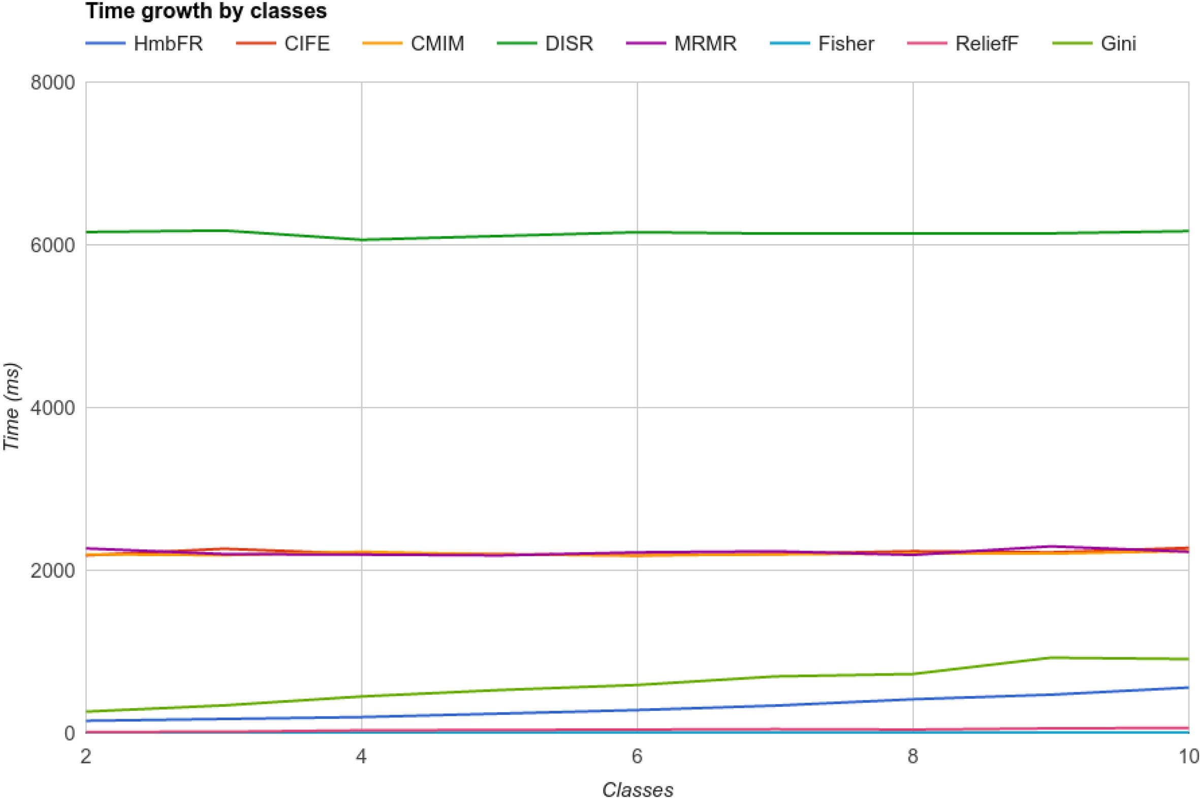

As we can see in Fig. 1, in terms of scalability due to increased number of classes, all reviewed algorithms handle the task very efficiently, at least complexity-order wise, we can identify 4 groups, DISR, which is not affected by class increase, but it’s quite slow, at least three times slower than other approaches such as CIFE, CMIM and MRMR all of which are not affected by class increase neither. A third group can be identified, Gini and HmbFR, both being slightly affected by class growth but not enough to fall even to a linear order scenario, finally a fourth group composed by ReliefF and Fisher, both performing very fast with no compromise in class size.

Next we continue with the analysis of sample growth.

Figure 2.

Scalability behavior for samples growth.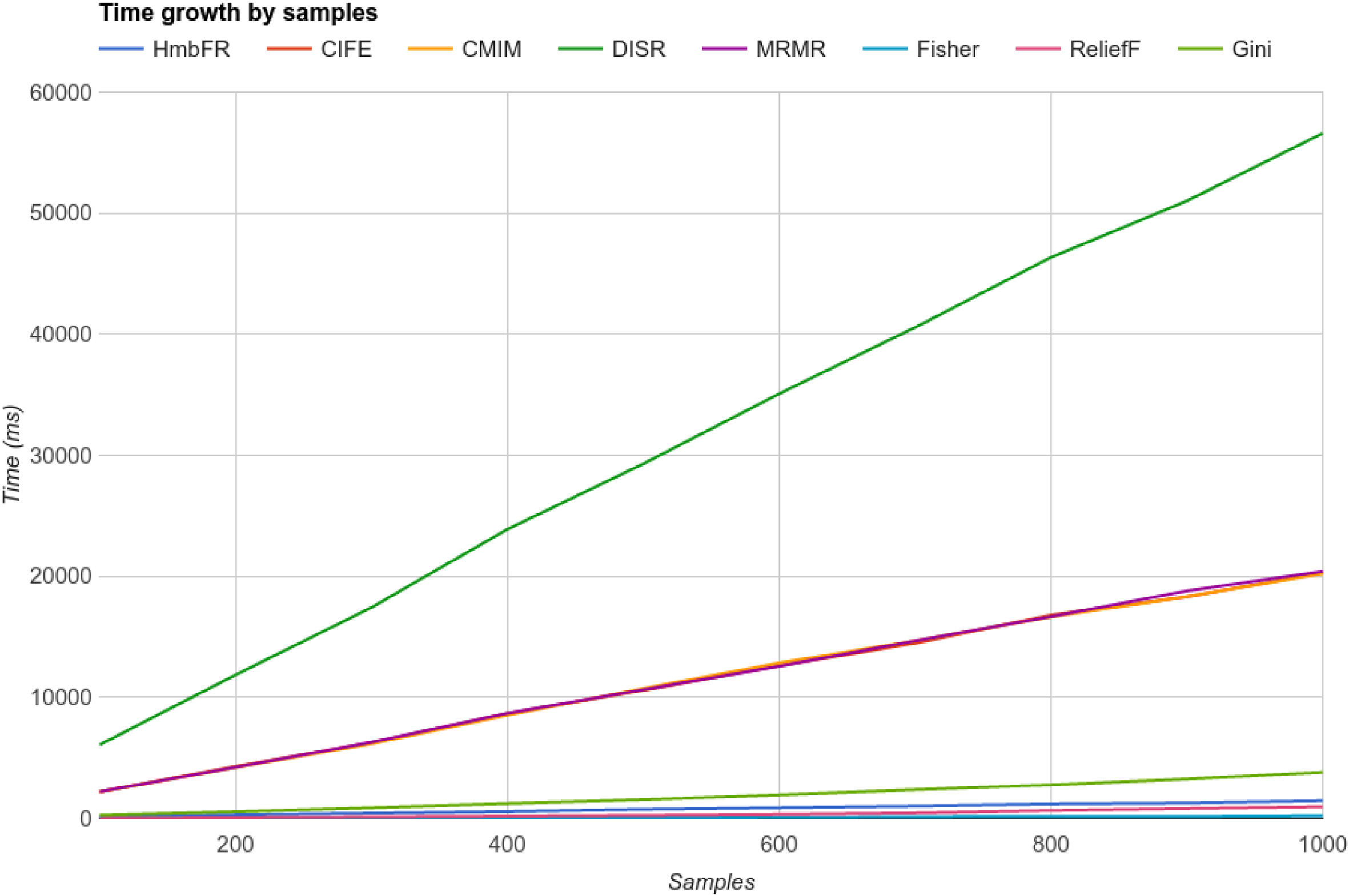

As far as samples increase, we can see in Fig. 2 most algorithms behave in a linear fashion, although some special cases need attention, once again DISR tops the time chart performing almost 300 hundred times slower than the fastest of the group, even scaling in a linear fashion. In terms of scalability issues, the worst scenario was for ReliefF which scaled at $n^{2}$ but since it performs very fast, it will require a very large number of samples to make it unfeasible.

Next, we review the case of features increase.

In Fig. 3 we can see the real issue with most algorithms, they scale at $n^{2}$ as the number of features increases, from the eight algorithms reviewed, half of them failed to keep a linear run time, only HmbFR, Fisher, ReliefF and Gini achieved to scale properly, hence they represent the only feasible option for real world test scenarios, where the number of features can easily reach 20,000 features or more. Table 2 summarizes this scalability evaluation.

Table 2

Summary of scale behavior

	Order
Algorithm	Classes	Samples	Features
HmbFR	$O(n)$	$O(n)$	$O(n)$
CIFE	$O(1)$	$O(n)$	$\bm{O(n^{2})}$
CMIM	$O(1)$	$O(n)$	$\bm{O(n^{2})}$
DISR	$O(1)$	$O(n)$	$\bm{O(n^{2})}$
MRMR	$O(1)$	$O(n)$	$\bm{O(n^{2})}$
Fisher	$O(1)$	$\bm{O(n\text{ log }n)}$	$O(n)$
ReliefF	$O(n)$	$\bm{O(n^{2})}$	$O(n)$
Gini	$O(n)$	$\bm{O(n\text{ log }n)}$	$O(n)$

Figure 3.

Scalability behavior for features growth.

We can see that half of the algorithms (CIFE, CMIM, DISR and MRMR) do not scale well as the number of features increases, with an $O(n^{2})$ order, those algorithms are really not suitable for high dimensional data. For our practical comparison we have selected the remaining four (HmbFR, Fisher, ReliefF and Gini), in Table 3 we show the characteristics of the benchmark datasets.

Table 3

Benchmark datasets details

Dataset	Classes	Samples	Features	Feat/Smp	Anomaly
Carcinom	11	174	9,182	55.8	0.330
Colon	2	62	2,000	32.3	0.485
GLI-85	2	85	22,283	262.1	0.234
Glioma	4	50	4,434	88.7	0.324
Leukemia	2	72	7,070	98.2	0.666
Lung	5	203	3,312	16.3	0.281
Orl-raws-10p	10	100	10,304	103.1	0.320
Prostate-ge	2	102	5,966	58.5	0.255
USPS	10	9298	256	0.03	0.252
Warp-pie-10p	10	210	2,420	11.5	0.296

In our experiments, most dataset easily exceed a thousand features, notable exception is the USPS dataset with only 256, but enough samples to cause troubles for algorithms such as ReliefF that scales quadratically with the number of samples. The need for more efficient algorithms is noticed more clearly when we consider high dimensional datasets such as GLI-85, with 22,283 features, trying to perform feature selection with algorithms such as DISR would be an infeasible task. We also include the feature to samples ratio to give an idea how disparity those values are, generally we would want more features if and only if those features are useful, otherwise, the less noise the better. To estimate how noisy the dataset is, we include the anomaly score as reported by IsolationForest [24] algorithm.

The benchmarking process consists of performing feature ranking for each dataset followed by a Stratified 10-fold cross validation that ensures class imbalance is considered in every fold. The whole process is repeated 10 times, every time using 10% fewer features (removing the less powerful ranked), this is done for 3 different classifiers as some datasets might favor a given learner. In total 300 setups are evaluated for every dataset using an F1 weighted (i.e, for each class) score to consider precision and recall in a single metric as Eq. (12) shows:

$\displaystyle F1=\frac{2*(\textit{precision}*\textit{recall})}{(\textit{% precision}+\textit{recall})}$ (12)

The Scikit-learn classifiers, as well as running parameters are being shown in Table 4.

Table 4

Classifiers setup

Classifier	Parameters
Naive bayes	Not required
Logistic regression	class_weight $=$ ‘balanced’, max_iter $=$ 200
Random forest	n_estimators $=$ Variable, class_weight $=$ ‘balanced’

The only parameter we carefully tuned was the number of estimators (or trees) for RandomForest using the formula in Eq. (13):

$\displaystyle n\_\textit{estimators}=10+\lceil\sqrt{\#_{\textit{feats}}}% \rfloor+\lceil\sqrt{\#_{\textit{Samples}}}\rfloor+\#_{\textit{Classes}}$ (13)

The rationale behind variable number of trees is that bigger and complex data sets usually need a higher number of trees, however, a higher number can be counterproductive for smaller scenarios and could lead to overfit.

In the following section, we present our analysis for each of the benchmarked dataset, as well as statistical significance analysis, this is done by comparing to a progressive linear reduction (PLR) algorithm, which only reduce features with no analysis involved, just linearly select a given amount. A t-test is performed against the PLR algorithm and the p-value is reported.

After feature reduction is completed, we take advantage of the smaller dimensionality dataset to enhance data representation. Given our reduced noise, we now use a 3 PCA vector representation that is being feed to an emergent self organized map (ESOM) [36] which will find a nonlinear representation in an unsupervised way that should provide an extra insight of dataset structure after noise has been reduced using only Top 10% of features as reported by HmbFR.

4.1 Carcinom

The Carcinom dataset has the most number of classes of our tests with 11, and with the only exception of the class 0, all others are nonlinearly separable in our 2D PCA representation as it can be seen in Fig. 4.

For this particular dataset Logistic Regression performed the best, achieving better performance across all number of selected features, these results can be seen in Table 5. Starting with a baseline score of $F1=$ 0.947 it was possible to increase the performance to 0.98 and 0.968 with Fisher and HmbFR respectively, both algorithms produce their best result with only 10% of the original features. On the other hand, ReliefF got a poor performance while Gini was not able to produce an acceptable p-value, therefore the results could fall under a lucky scenario.

Table 5
Logistic Regression for Carcinom

Num. Features	HmbFR	Fisher	ReliefF	Gini	PLR
9182	0.947	0.947	0.947	0.947	0.947
8264	0.947	0.955	0.939	0.929	0.929
7346	0.953	0.960	0.944	0.919	0.939
6427	0.944	0.970	0.944	0.929	0.939
5509	0.955	0.972	0.936	0.938	0.903
4591	0.951	0.977	0.936	0.945	0.918
3673	0.960	0.977	0.941	0.936	0.917
2755	0.960	0.980	0.951	0.929	0.923
1836	0.960	0.980	0.951	0.918	0.910
918	0.968	0.980	0.957	0.916	0.894
Average	0.955	0.970	0.945	0.931	0.922
Peak	0.968	0.980	0.957	0.947	0.947
PLR p-value	0.002	0.000	0.005	0.142	NA

Figure 4.

Carcinom visualization.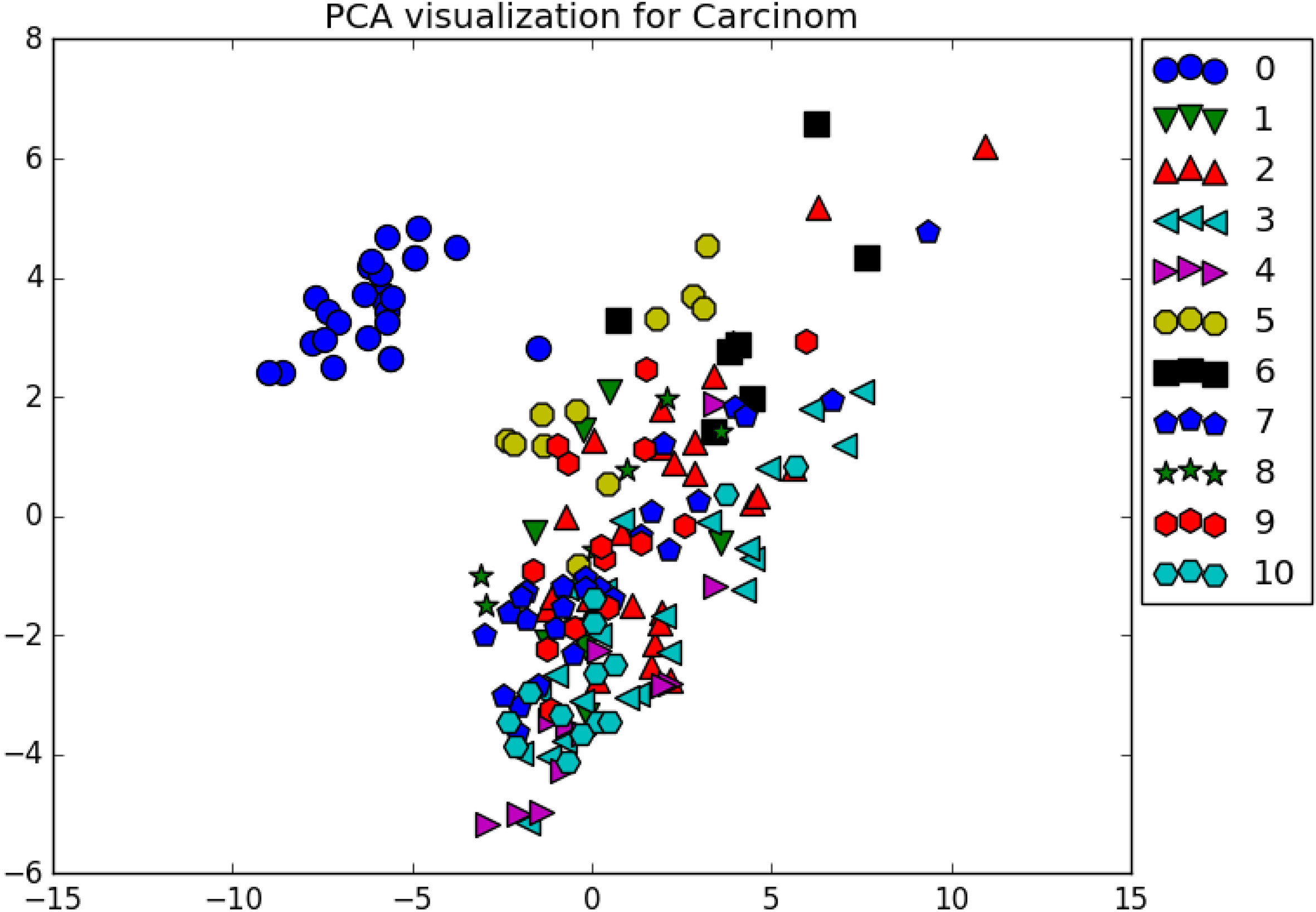

Figure 5.

Carcinom reduced features SOM plane.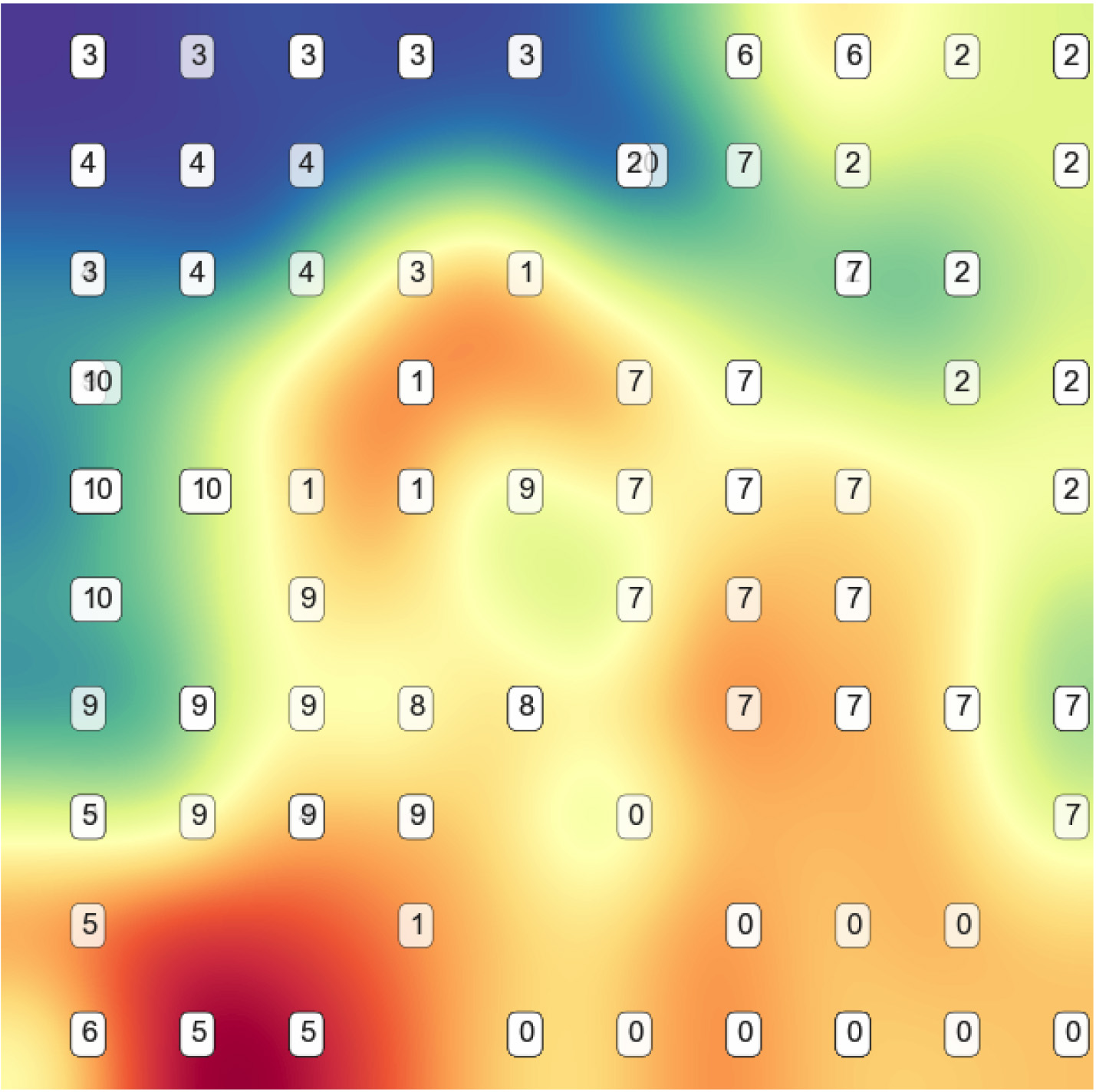

Figure 6.

Colon visualization.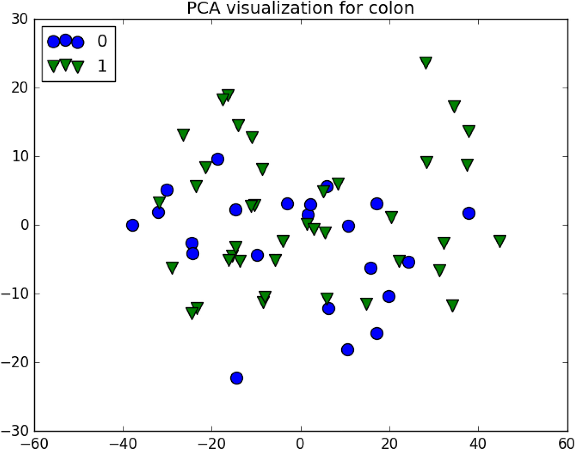

Using only 10% of the original features, it was possible to improve in 2% the baseline model, although at minimal improvement, we can see in Fig. 5 that the ESOM plane makes much better job at separating the instances while still maintaining a similar structure, for instance, classes No. 5 and 0 are very similar spaced as they were in the original PCA plot but now have better margins vs other classes.

4.2 Colon

The colon dataset looks simple to separate (see Fig. 6), a single decision tree might do a very good job on its own, and with only two classes its not surprise that Random Forest performed the best in this scenario.

An interesting result (Table 6) arise from the colon dataset, all algorithms achieved a very high p-value, meaning that for this dataset with so few features (2000), feature reduction might be trivial, ReliefF and HmbFR achieved the best peak result with 0.865 and 0.851 although HmbFR seems a bit more stable with a better average score. Fisher and Gini performed poorly in this task with a score even lower than PLR.

Table 6
Random forest for colon

Num. Features	HmbFR	Fisher	ReliefF	Gini	PLR
2000	0.817	0.817	0.817	0.817	0.817
1800	0.817	0.790	0.819	0.803	0.786
1600	0.790	0.789	0.774	0.815	0.786
1400	0.768	0.803	0.774	0.776	0.790
1200	0.833	0.803	0.818	0.771	0.848
1000	0.831	0.833	0.814	0.831	0.831
800	0.846	0.836	0.833	0.832	0.831
600	0.851	0.832	0.832	0.814	0.790
400	0.850	0.818	0.865	0.818	0.801
200	0.846	0.821	0.865	0.832	0.859
Average	0.825	0.814	0.821	0.811	0.814
Peak	0.851	0.836	0.865	0.832	0.859
PLR p-value	0.245	0.963	0.474	0.762	NA

Figure 7.

Colon reduced features SOM plane.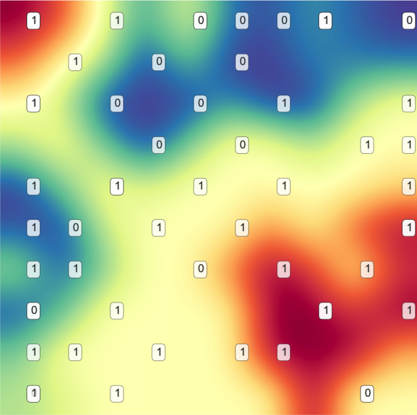

With a 3% improvement in model performance, and after removing 90% of the original features, the visualization of the Colon dataset is dramatically improved by the ESOM plane, while the PCA plot hardly separates the classes, the new representation shows a clear separation as seen in Fig. 7.

4.3 GLI-85

The GLI-85 dataset has the most potential for feature reduction, given the over 22,000 features and the dataset characteristics, it seems some parts of the data are linearly separable as we can see in its PCA visualization in Fig. 8.

As expected from the PCA analysis, all algorithms seems to be improving classification performance when Logistic Regression is used (Table 7), the reductions are very good, using only 10% of the original features ( $\approx 2k$ vs $\approx 20k$ ) seems to improve by as much as 4% with HmbFR or 5% by Fisher and ReliefF. In this particular dataset our approach did not succeed in improving over other techniques, however, it remains very competitive and a low p-value gives confidence on its performance.

Table 7
Logistic regression for GLI-85

Num. Features	HmbFR	Fisher	ReliefF	Gini	PLR
22283	0.886	0.886	0.886	0.886	0.886
20055	0.886	0.900	0.897	0.900	0.886
17826	0.886	0.911	0.900	0.900	0.886
15598	0.897	0.911	0.911	0.900	0.897
13370	0.912	0.912	0.911	0.912	0.886
11142	0.886	0.912	0.911	0.912	0.886
8913	0.912	0.912	0.923	0.912	0.886
6685	0.912	0.936	0.936	0.925	0.897
4457	0.925	0.936	0.936	0.925	0.911
2228	0.925	0.936	0.925	0.925	0.878
Average	0.903	0.915	0.914	0.910	0.890
Peak	0.925	0.936	0.936	0.925	0.911
PLR p-value	0.033	0.001	0.001	0.001	NA

Figure 8.

GLI-85 visualization.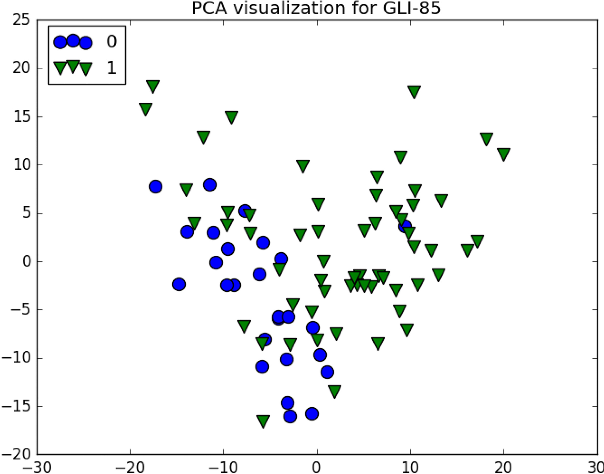

Using only 10% of the original features helped to boost the model performance 4%, the dataset is a bit unbalanced in favor of positive class and so can be noticed for both the PCA and the ESOM plots. However, after reduction, we can see a much clearer representation, although some outliers are still present as seen in Fig. 9.

Figure 9.

GLI-85 reduced features SOM plane.

4.4 Glioma

The Glioma dataset represents a huge challenge for feature selection, as there are way too many classes (4) for a very small number of samples (50) as it can be seen in Fig. 10, to make the scenario worse, the classes are all merged with no apparent linear separability.

According to p-values in Table 8, Fisher is the more likely to be different than the simple PLR, however it felt short as peak performance regards, running behind Gini and HmbFR with 0.821 and 0.815 however, each algorithm reached that score with a very different set of features, while Gini required 90% of the original space, HmbFR used only 60%. The average score is improved for all algorithms vs PLR.

Table 8
Random forest for Glioma

Num. Features	HmbFR	Fisher	ReliefF	Gini	PLR
4434	0.772	0.772	0.772	0.772	0.772
3991	0.748	0.753	0.785	0.821	0.767
3547	0.747	0.783	0.758	0.787	0.740
3104	0.805	0.764	0.699	0.787	0.751
2660	0.815	0.807	0.759	0.772	0.753
2217	0.755	0.778	0.790	0.773	0.795
1774	0.759	0.770	0.742	0.766	0.760
1330	0.686	0.780	0.775	0.683	0.734
887	0.742	0.717	0.686	0.725	0.675
443	0.777	0.782	0.768	0.735	0.721
Average	0.760	0.771	0.753	0.762	0.747
Peak	0.815	0.807	0.790	0.821	0.795
PLR p-value	0.337	0.028	0.477	0.187	NA

Figure 10.

Glioma visualization.

For the Glioma dataset, best reduction threshold seems to be around 70% of original features, however, to help reduce potential noise, we still keep only 10% of the data for build the ESOM planes, in this case, using 443 features which still provides an improvement vs the base model. From the original PCA plot, we can see classes 0 and 1 are overlapped as well as 2 and 3. However, in the ESOM plane, we can a see a more clear separation as shown in Fig. 11.

Figure 11.

Glioma reduced features SOM plane.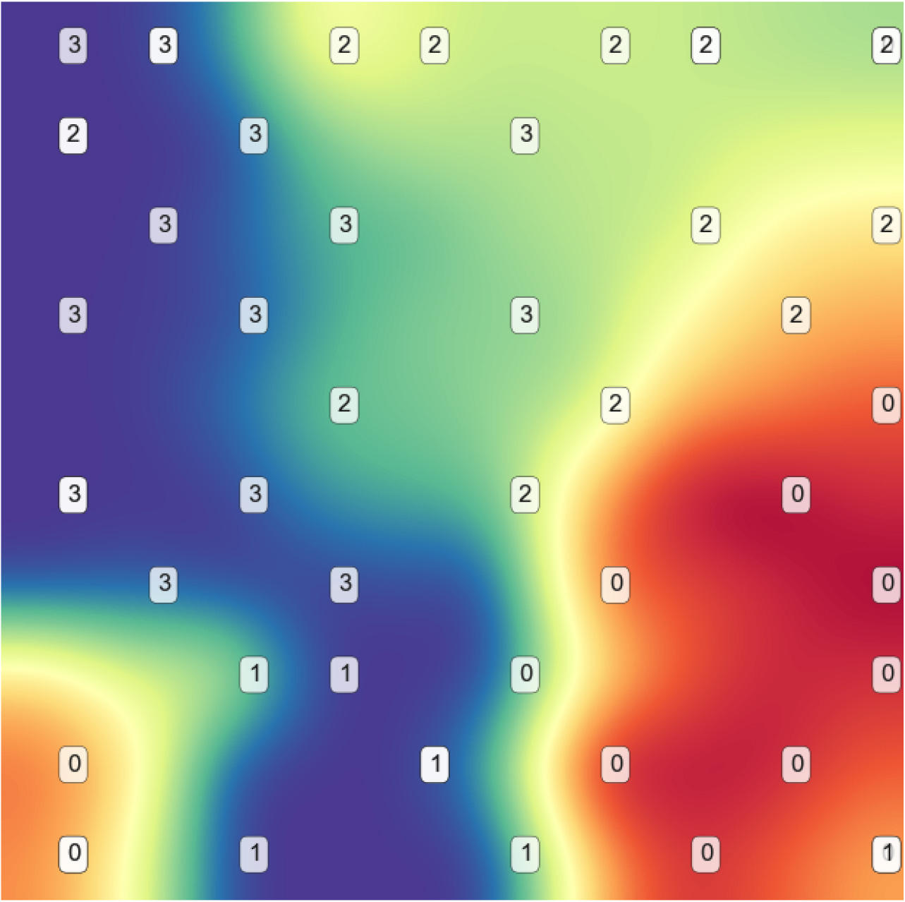

4.5 Leukemia

The Leukemia dataset looks complex for feature selection, with 72 instances and over 7,000 features, the chances of overfitting are huge, however as we can see from the PCA plot in Fig. 12, the data does not seem too hard to separate.

Figure 12.

Leukemia visualization.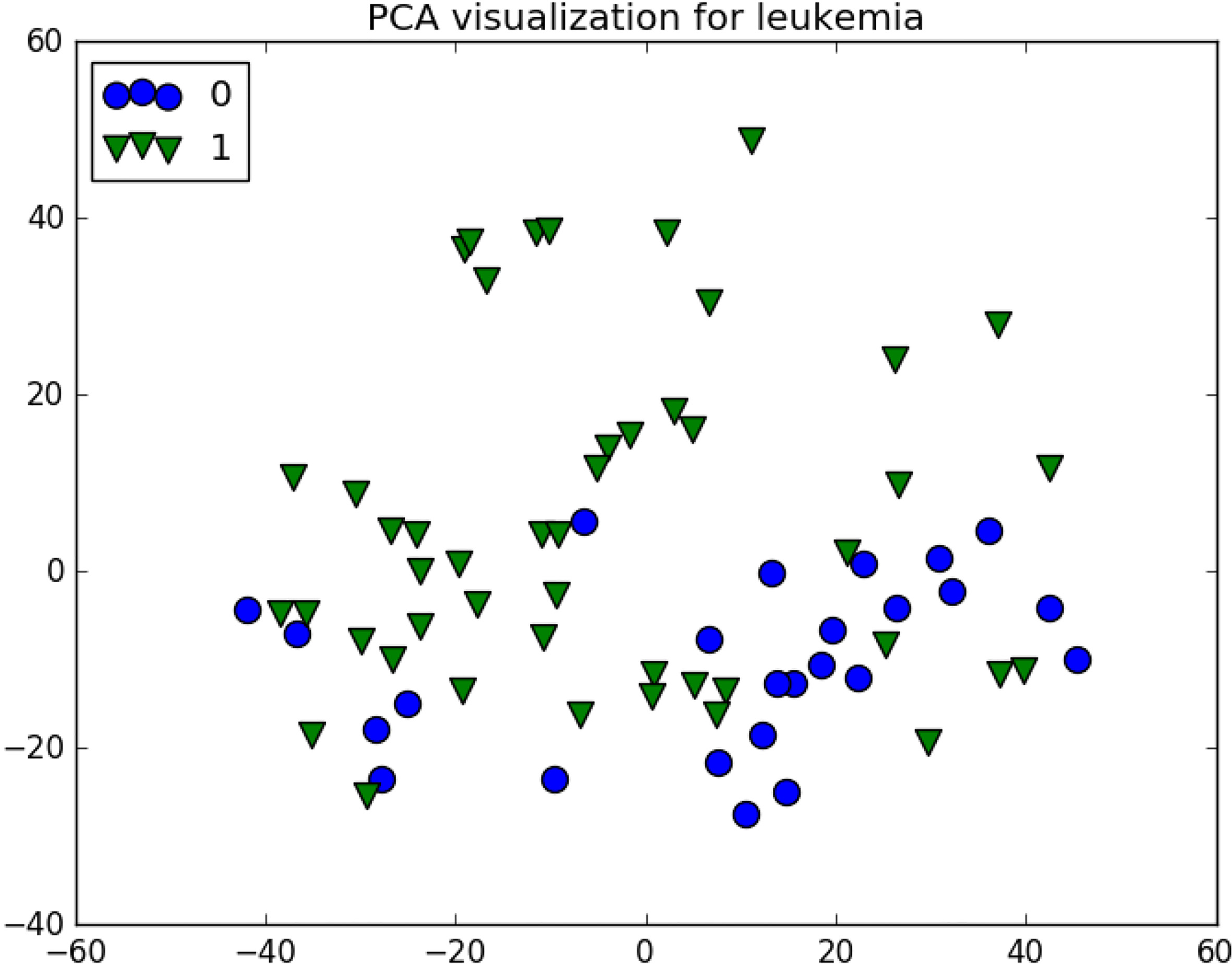

For this particular dataset Random Forest performed the best, with an impressive baseline performance of over 0.93 without any feature selection as shown in Table 9. It seems that the practical best possible score is 0.981 as all algorithms stuck in that mark, the PLR, in this case, performed way lower than the benchmark algorithms, all of them producing a much higher average score.

Table 9

Random forest for Leukemia

Num. Features	HmbFR	Fisher	ReliefF	Gini	PLR
7070	0.934	0.934	0.934	0.934	0.934
6363	0.949	0.981	0.981	0.934	0.947
5656	0.926	0.952	0.963	0.931	0.918
4949	0.906	0.963	0.981	0.968	0.950
4242	0.981	0.937	0.981	0.968	0.965
3535	0.965	0.981	0.950	0.963	0.952
2828	0.963	0.947	0.968	0.981	0.889
2121	0.981	0.981	0.963	0.981	0.902
1414	0.965	0.981	0.981	0.981	0.885
707	0.963	0.981	0.981	0.981	0.763
Average	0.953	0.964	0.969	0.962	0.911
Peak	0.981	0.981	0.981	0.981	0.965
PLR p-value	0.079	0.036	0.020	0.047	NA

In this dataset the classes are overlapped due to structure complexity, but also imbalance, a 3% increase in model performance is achieved after using only 10% of the original features, this reduction is also beneficial to visualization, as we can see in Fig. 13, although some overlap still exist, there is a better separation overall.

Figure 13.

Leukemia reduced features SOM plane.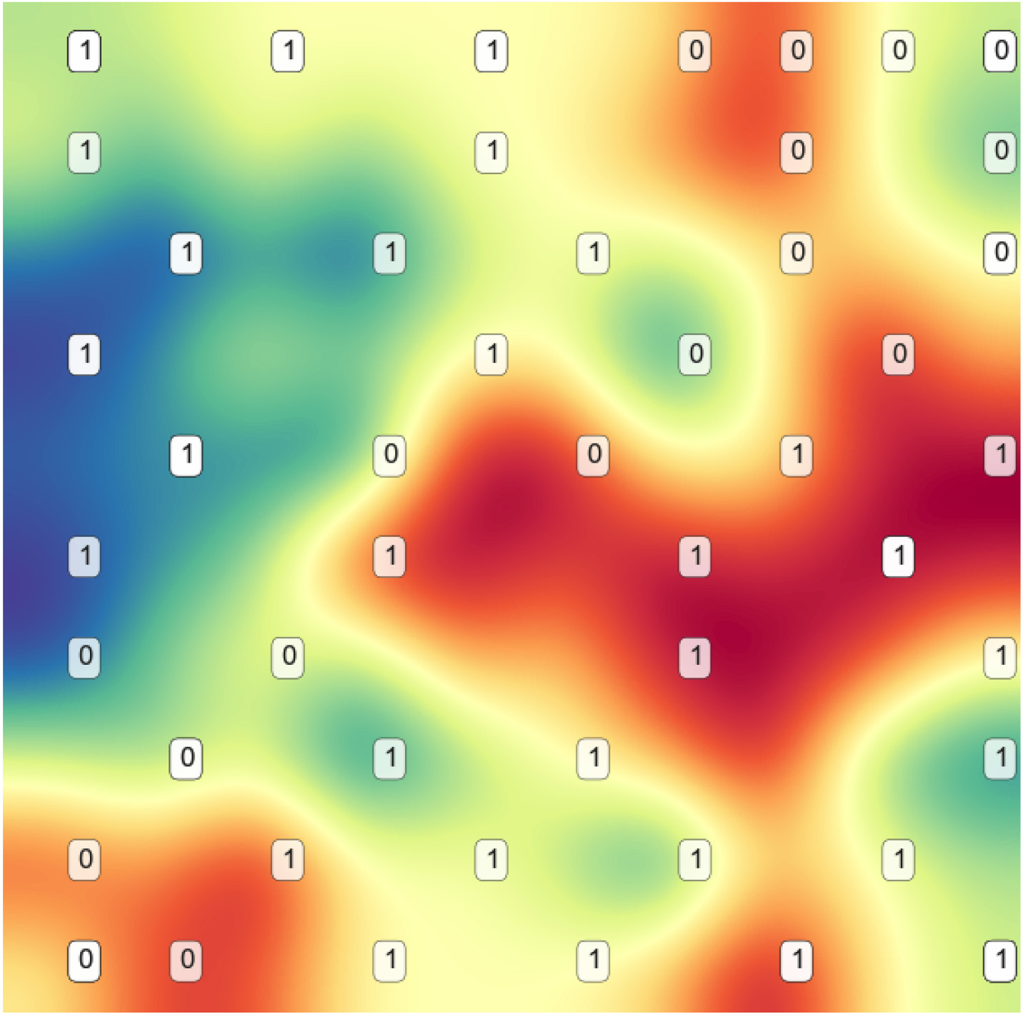

4.6 Lung

The Lung dataset is a challenge because it has many classes for a relative number of samples and features, in this particular case, more features would have benefited the data in order to improve separability especially for class 0 and 4 as can be seen in the PCA representation in Fig. 14.

After analysing results presented in Table 10, it seemed that the best practical score could be 0.976 as three algorithms stuck in such mark, however HmbFR managed to find a combination of features capable of 0.98, interesting enough, this combination is also with a smaller set of features of only 10% of the original data, the closest competition comes from Fisher, performing not only slightly less powerful but also requiring 60% of the original data. Averages and p-values are low enough across all methods.

Table 10
Logistic regression for Lung

Num. Features	HmbFR	Fisher	ReliefF	Gini	PLR
3312	0.976	0.976	0.976	0.976	0.976
2981	0.976	0.976	0.976	0.976	0.976
2650	0.976	0.976	0.976	0.976	0.976
2318	0.976	0.976	0.969	0.976	0.965
1987	0.976	0.976	0.969	0.976	0.965
1656	0.976	0.972	0.969	0.976	0.959
1325	0.970	0.972	0.969	0.965	0.964
994	0.976	0.972	0.965	0.965	0.957
662	0.965	0.972	0.965	0.969	0.952
331	0.980	0.959	0.965	0.972	0.921
Average	0.974	0.972	0.970	0.972	0.961
Peak	0.980	0.976	0.976	0.976	0.976
PLR p-value	0.038	0.013	0.063	0.045	NA

Figure 14.

Lung visualization.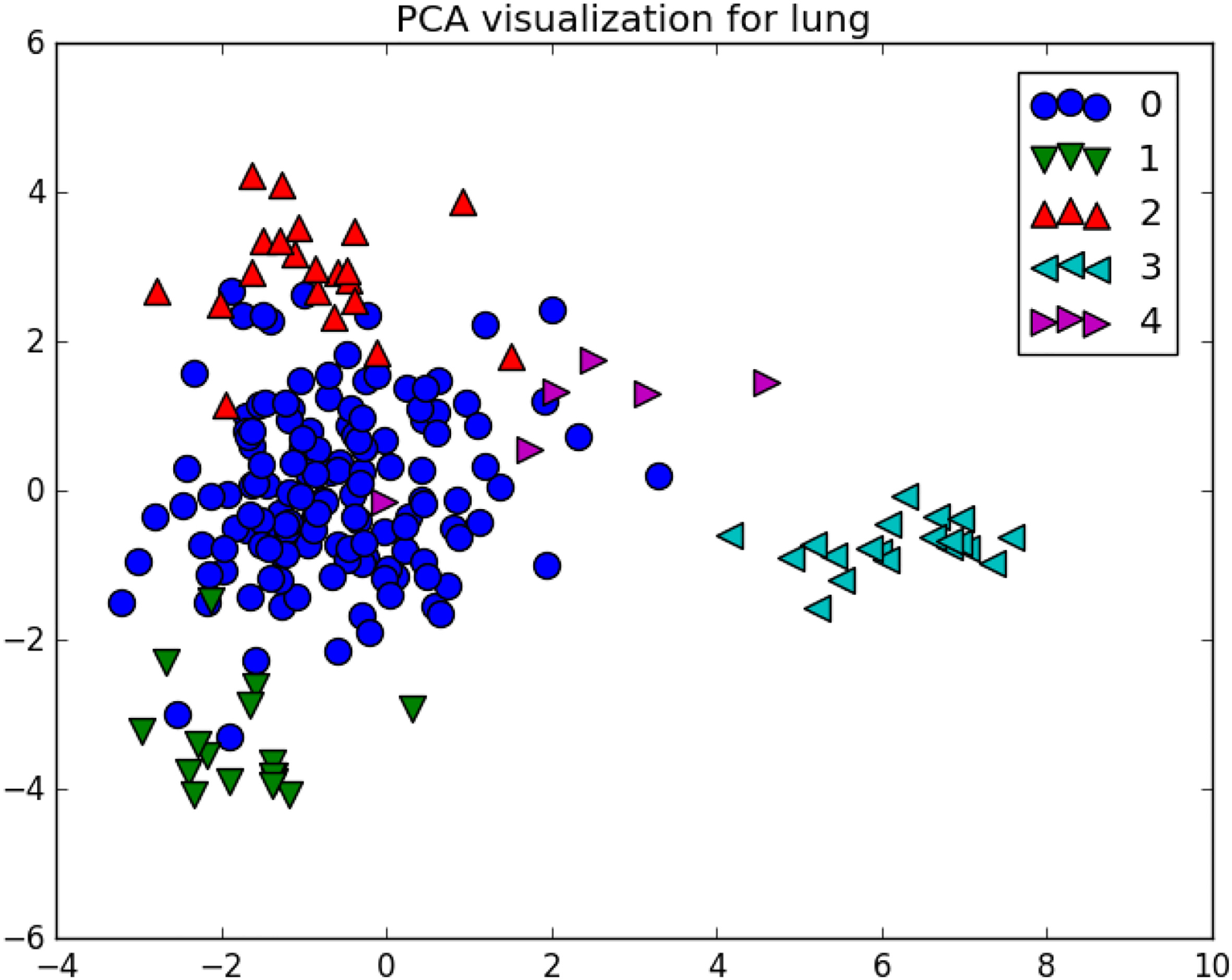

In this particular case HmbFS using only 10% of the features achieved the best overall performance, which can be a signal for very high improvements in visualization, starting with the original PCA, we can see class 0 dominating the plot and causing heavy overlap. In the ESOM plane (Fig. 15), the class separation is dramatically improved, for instance, class 1 and 0 that were previously overlapped now are fully separated.

Figure 15.

Lung reduced features SOM plane.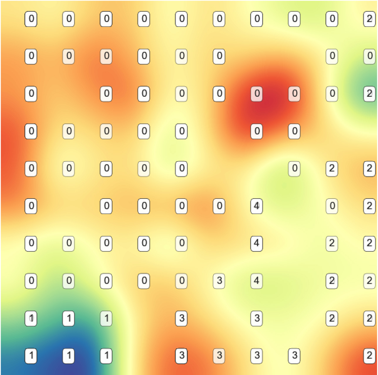

4.7 Orl-raws-10p

This dataset, being constructed by face images adds a new scenario for the benchmark, using pixels as features, the ORL face data has over 10,000 features to describe 10 classes (persons). The PCA analysis in Fig. 16 suggests that there is indeed some linear separability.

Figure 16.

ORL raws 10p visualization.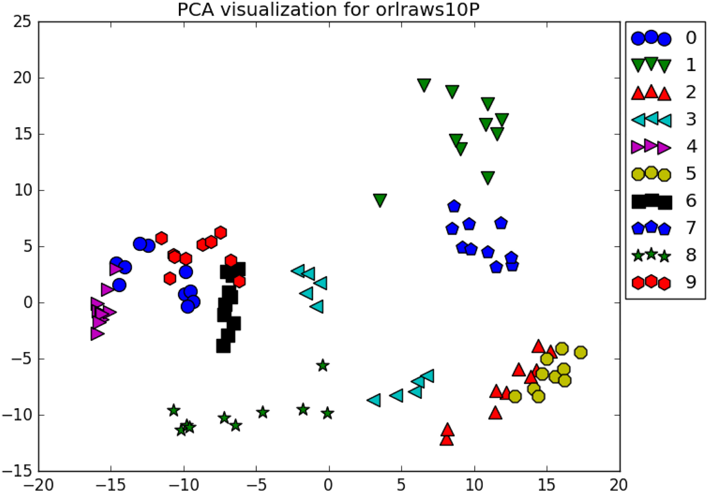

As expected from the data overview, it can be easily separated even without feature selection for a very powerful 0.967 baseline score as shown in Table 11. Notable, all algorithms managed to find a subset of features that improved such score, best two were HmbFR and Fisher, improving the recognition by 2% or in some cases a perfect F-Score by Fisher, the p-value, however, is much lower for HmbFR which seems to produce more stable results.

Table 11

Logistic regression for ORL

Num. Features	HmbFR	Fisher	ReliefF	Gini	PLR
10304	0.967	0.967	0.967	0.967	0.967
9274	0.967	0.967	0.967	0.973	0.967
8243	0.967	0.967	0.967	0.973	0.967
7213	0.967	0.967	0.967	0.973	0.967
6182	0.967	0.967	0.973	0.973	0.967
5152	0.973	0.967	0.967	0.973	0.967
4122	0.987	0.967	0.967	0.973	0.973
3091	0.960	0.973	0.973	0.933	0.960
2061	0.973	0.973	0.947	0.887	0.947
1030	0.973	1.000	0.977	0.847	0.877
Average	0.970	0.971	0.967	0.947	0.956
Peak	0.987	1.000	0.977	0.973	0.973
PLR p-value	0.168	0.236	0.286	0.280	NA

Given the very little class overlap for the ORL dataset, improvement in model performance was limited to only 0.6% when using 10% of best features as ranked by HmbFR. The ESOM produced an overall good structure visualization as seen in Fig. 17, however, for this specific case, the PCA plot seems to provide a better overview, a signal that feature reduction might not always give an improvement.

Figure 17.

ORL reduced features SOM plane.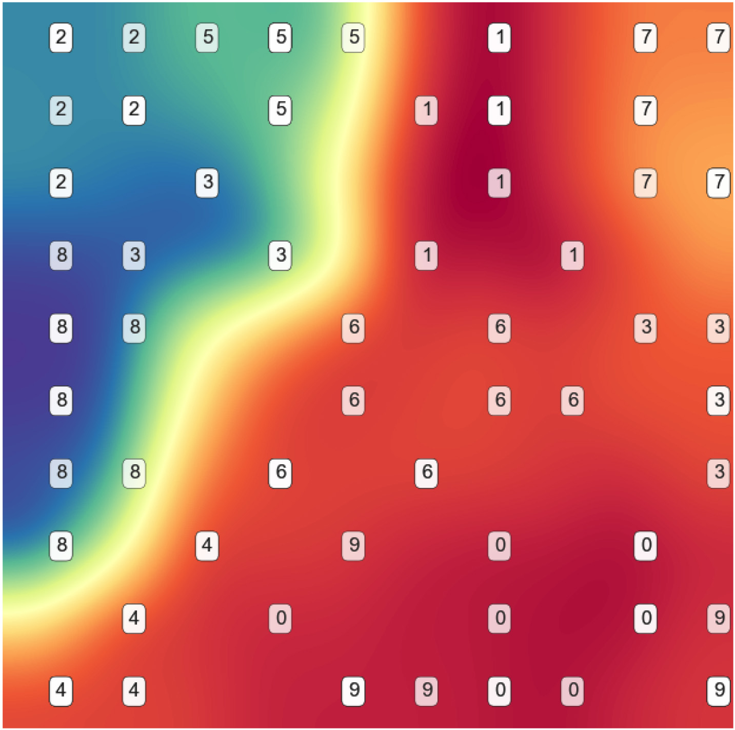

4.8 Prostate-ge

The prostate dataset has enough features to separate the binary classes with a very good performance as seen in Fig. 18, however, since some samples have heavy overlap, it is possible to reach a point where improvements become very hard.

For this datasets, all algorithms achieved a very low p-value as the baseline PLR performed very poorly doing progression reduction as shown in Table 12. It is worth noting how from 100% to 60% of features, most algorithms kept the original performance, except ReliefF which produced a good performance improvement. Best two approaches were HmbFR and ReliefF, with 0.939 and 0.95, both of them achieved such results with a very low number of features, 20% and 10% respectively.

Table 12
Logistic regression for Prostate-Ge

Num. Features	HmbFR	Fisher	ReliefF	Gini	PLR
5966	0.911	0.911	0.911	0.911	0.911
5369	0.911	0.911	0.920	0.911	0.911
4773	0.920	0.911	0.920	0.911	0.911
4176	0.910	0.910	0.930	0.911	0.911
3580	0.910	0.910	0.940	0.911	0.911
2983	0.920	0.920	0.940	0.911	0.891
2386	0.920	0.929	0.940	0.920	0.891
1790	0.920	0.929	0.940	0.929	0.891
1193	0.939	0.929	0.950	0.929	0.821
597	0.929	0.929	0.950	0.929	0.826
Average	0.919	0.919	0.934	0.917	0.888
tabst Peak	0.939	0.929	0.950	0.929	0.911
PLR p-value	0.049	0.044	0.011	0.054	NA

Figure 18.

Prostate GE visualization.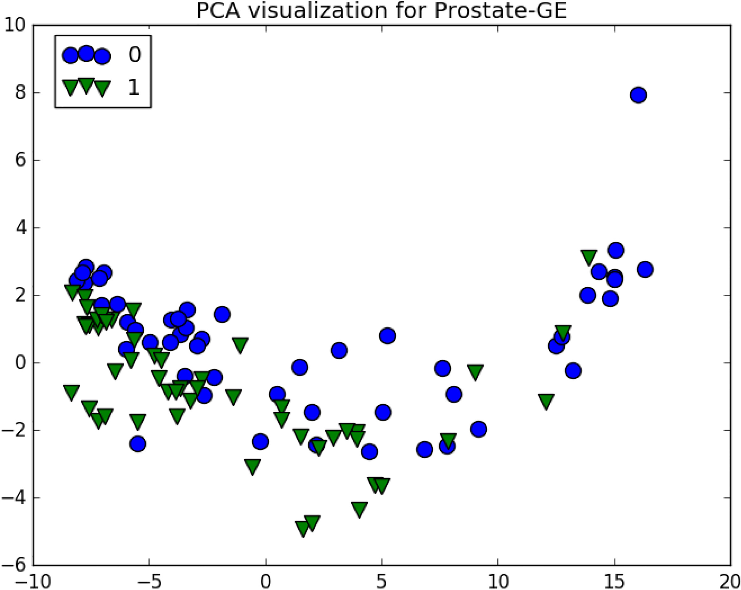

The prostate dataset gained around 2% when a 90% of features got removed, based on the original PCA representation, both classes are heavily merged, however in the ESOM plane as can be seen in Fig. 19, there is a very clear separation of classes with very minimal overlapping.

Figure 19.

Prostate reduced features SOM plane.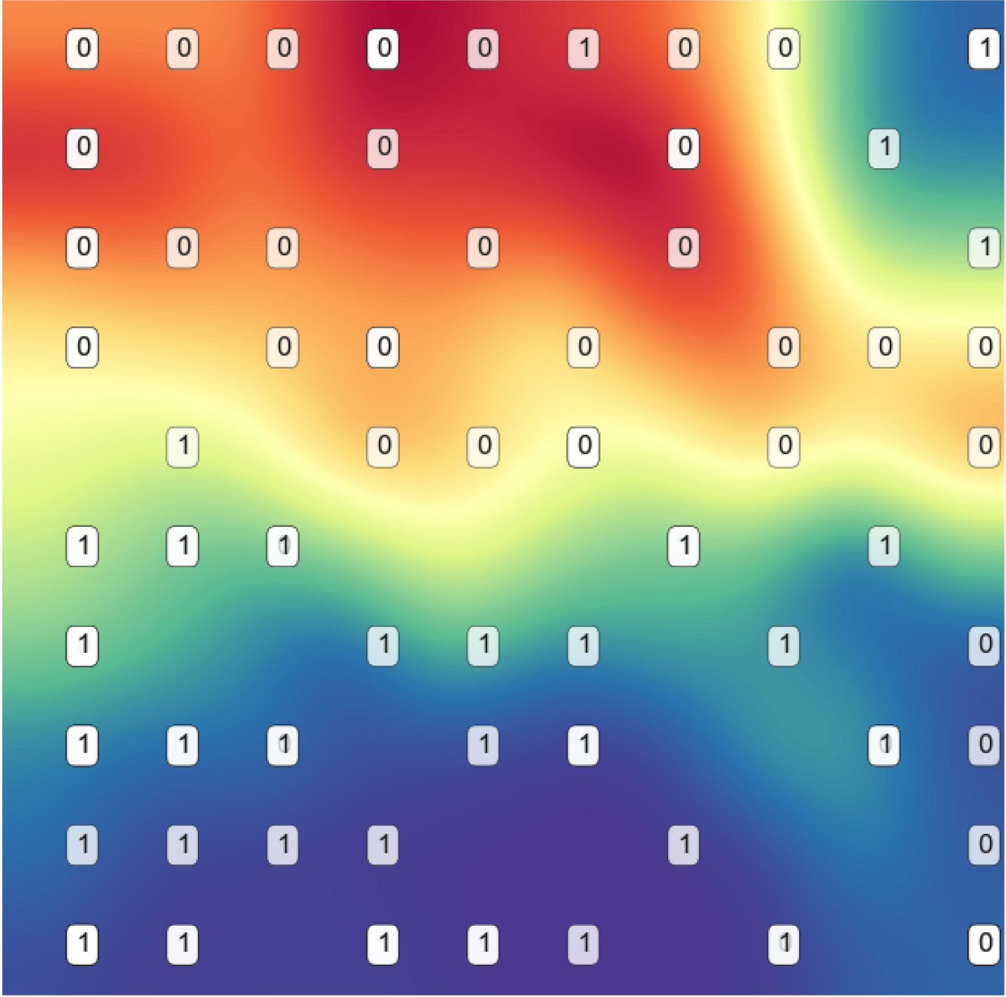

4.9 USPS

Just by looking at the PCA plot in Fig. 20, the USPS dataset is clearly a nice add-on to the benchmarks as it is very different, having almost 10,000 samples of hand written digits with a 16 $\times$ 16 resolution (hence 256 features) and 10 different classes, is a nice challenge for feature interactions and reduction. We can see how all classes are sort of merged all over spectrum so linear separability seems very unlikely.

Figure 20.

USPS visualization.

For this particular dataset, it was possible to achieve 0.945 using Logistic Regression and 0.961 using Random Forest (RF), however, after using feature selection (FS) the results only got worse, although HmbFR achieved as high as 0.851 with RF using only 10% of features. For this analysis, we selected Naive Bayes (NB) as it indeed benefits from FS as we can see in Table 13. From the results table, it is clear how feature reduction is not trivial, PLR achieved scores as low as 0.327 where other techniques such as HmbFR using the same 10% of features achieved 0.685. Gini performed poorly in this case, while the two best were HmbFR and ReliefF, both of them with improvements over 8% and interesting enough, both of them achieved the peak performance with the same number of features at 50%.

Table 13

Naive bayes for USPS

Num. Features	HmbFR	Fisher	ReliefF	Gini	PLR
256	0.783	0.783	0.783	0.783	0.783
230	0.811	0.799	0.811	0.763	0.787
205	0.829	0.820	0.844	0.754	0.795
179	0.859	0.843	0.864	0.709	0.773
154	0.869	0.842	0.874	0.661	0.761
128	0.870	0.835	0.877	0.606	0.703
102	0.856	0.838	0.857	0.620	0.630
77	0.795	0.798	0.836	0.616	0.525
51	0.771	0.766	0.792	0.575	0.389
26	0.685	0.631	0.707	0.494	0.327
Average	0.813	0.795	0.825	0.658	0.647
Peak	0.870	0.843	0.877	0.783	0.795
PLR p-value	0.004	0.007	0.004	0.747	NA

Figure 21.

USPS reduced features SOM plane.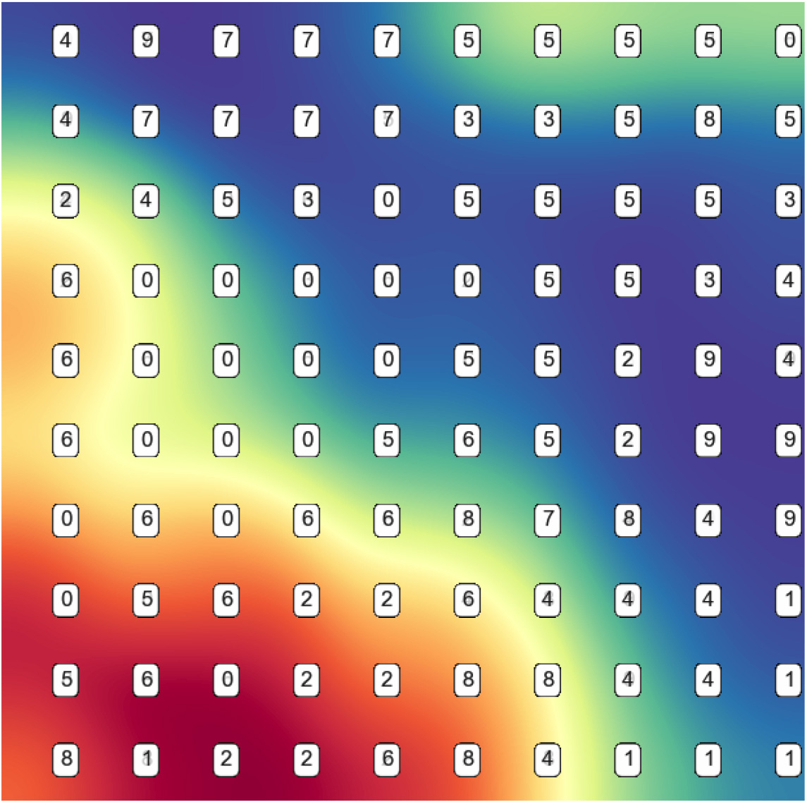

The USPS dataset is our biggest data in term of instances but the smallest in term of features, which means that most instances look very similar, and are all overlapped at least in a 2 dimensions space, after reduction to only 26 features and then building the ESOM plane (Fig. 21), the data seems a bit better represented but not enough to overcome the extra processing required.

4.10 Warp-pie-10p

Looking at the data it’s clear that linear separability is challenging, with so many classes and no apparent cluster regions as all classes are mixed together as we can see in Fig. 22, feature selection algorithms will be required to careful rank the features.

For this particular dataset, Logistic Regression performed a bit better, however, no useful conclusion could be made as feature selection (FS) did not provide any improvement, however, for Naive Bayes, the improvement is clear and low p-values support this improvement (see Table 14). Best algorithm was HmbFR with a 0.963 score, improving 3% over the baseline without FS using only 20% of the data, another notable result comes from Fisher, with a 0.955 score although using 30% of data.

Table 14
Naive bayes for Warp pie 10p

Num. Features	HmbFR	Fisher	ReliefF	Gini	PLR
2420	0.934	0.934	0.934	0.934	0.934
2178	0.937	0.940	0.924	0.937	0.910
1936	0.943	0.940	0.922	0.915	0.916
1694	0.946	0.943	0.920	0.891	0.906
1452	0.938	0.947	0.908	0.827	0.854
1210	0.939	0.952	0.916	0.719	0.833
968	0.955	0.951	0.926	0.751	0.792
726	0.956	0.955	0.934	0.761	0.776
484	0.963	0.952	0.948	0.709	0.744
242	0.942	0.946	0.942	0.630	0.755
Average	0.945	0.946	0.927	0.807	0.842
Peak	0.963	0.955	0.948	0.937	0.934
PLR p-value	0.003	0.002	0.008	0.053	NA

Figure 22.

Warp pie 10p visualization.

In this case, the original 2-dimensional representation is highly overlapped, as a similar scenario as USPS, however in this case, with much more features, noise reduction was actually beneficial, improving 2% with only 10% of the original space. The ESOM plane in Fig. 23 shows a huge improvement over the original data representation even when it shows some minor overlap.

Figure 23.

Warp reduced features SOM plane.

5. Conclusions and future work

Nowadays, we have powerful classifiers with built-in feature selection, however, for high dimensional spaces, there is still a lot of work to be done. As shown in our experiments, feature selection algorithms are pushing the performance of the classifiers in every case.

Based on our results, it is clear that the problem of feature selection is still dependent on the data structure, and there is no single best algorithm, however, for our particular setup, it seems that HmbFR and Fisher are more stable across different setups while Gini did not perform well with these datasets.

In general, our approach proved to be competitive with current algorithms while ranking in a compressed space and no evaluation of individual features required.

Data visualization is also an added benefit of feature selection, once space is reduced and only the best features are kept we are able to build more exhaustive dimensionality reduction techniques such as emergent self-organizing maps which proved to be a very effective approach.

Regarding our feature work, we can divide our efforts into two main paths, performance and enhancements. First, with the surge of powerful GPU, our heat map generation is a good fit for intensive parallelization which would allow stacking of heat maps to improve performance. Second, in sensitive applications, the raw performance improvement is negligible if it can not be properly explained, therefore given algorithm design, we plan to use our heat map as a visual aid to integrate Human-in-the-loop (HITL) in the selection process.

Footnotes

Acknowledgments

Conacyt – Maestria y Doctorado en Ciencia e Ingenieria.

References

Akadi

A.E.

Ouardighi

A.E.

and Aboutajdine

, A powerful feature selection approach based on mutual information, International Journal of Computer Science and Network Security (2008), 116–121.

Alelyani

, On Feature Selection Stability: A Data Perspective, PhD thesis, Tempe, AZ, USA, 2013. AAI3558275.

Battiti

, Using mutual information for selecting features in supervised neural net learning, Trans. Neur. Netw. 5(4) (July 1994), 537–550.

Blum

A.L.

and Langley

, Selection of relevant features and examples in machine learning, Artif. Intell. 97(1–2) (Dec. 1997), 245–271.

Brown

Pocock

Zhao

M.-J.

and Luján

, Conditional likelihood maximisation: A unifying framework for information theoretic feature selection, J. Mach. Learn. Res. 13(1) (Jan. 2012), 27–66.

Das

, Filters, wrappers and a boosting-based hybrid for feature selection, in: Proceedings of the Eighteenth International Conference on Machine Learning, San Francisco, CA, USA, 2001, ICML ’01, Morgan Kaufmann Publishers Inc., pp. 74–81.

Dash

and Liu

, Feature selection for classification, Intelligent Data Analysis 1 (1997), 131–156.

Deng

Berg

and Fei-Fei

, Hierarchical semantic indexing for large scale image retrieval, in: Computer Vision and Pattern Recognition (CVPR), 2011 IEEE Conference on, June 2011, pp. 785–792.

Duda

R.O.

Hart

P.E.

and Stork

D.G.

, Pattern Classification (2Nd Edition), Wiley-Interscience, 2000.

10.

Fleuret

, Fast binary feature selection with conditional mutual information, J. Mach. Learn. Res. 5 (Dec. 2004), 1531–1555.

11.

Forman

, An extensive empirical study of feature selection metrics for text classification, J. Mach. Learn. Res. 3 (Mar. 2003), 1289–1305.

12.

Golub

and Van Loan

, Matrix Computations, Matrix Computations, Johns Hopkins University Press, 2012.

13.

and Han

, Generalized fisher score for feature selection, CoRR abs/1202.3725 (2012).

14.

Eils

and Schlesner

, Complex heatmaps reveal patterns and correlations in multidimensional genomic data, Bioinformatics 32(18) (2016), 2847–2849.

15.

Guyon

and Elisseeff

, An introduction to variable and feature selection, J. Mach. Learn. Res. 3 (Mar. 2003), 1157–1182.

16.

Hastie

T.J.

Tibshirani

R.J.

and Friedman

J.H.

, The elements of statistical learning : data mining, inference, and prediction, Springer series in statistics, Springer, New York, 2009. Autres impressions: 2011 (corr.), 2013 (7e corr.).

17.

Huertas

and Juárez-Ramírez

, Heat map based feature selection: A case study for ovarian cancer, in: Applications of Evolutionary Computation – 18th European Conference, EvoApplications 2015, Copenhagen, Denmark, April 8–10, 2015, Proceedings, 2015, pp. 3–13.

18.

Hughes

, On the mean accuracy of statistical pattern recognizers, IEEE Transactions on Information Theory 14(1) (Jan 1968), 55–63.

19.

Jain

and Chandrasekaran

, Dimensionality and sample size considerations, in: Pattern Recognition in Practice Krishnaiah

and Kanal

, eds, 1982, pp. 835–855.

20.

John

G.H.

Kohavi

and Pfleger

, Irrelevant features and the subset selection problem, in: Machine Learning: Proceedings of the Eleventh International, Morgan Kaufmann, 1994, pp. 121–129.

21.

Kohavi

and John

G.H.

, Wrappers for feature subset selection, Artif. Intell. 97(1–2) (Dec. 1997), 273–324.

22.

Cheng

Wang

Morstatter

Trevino

R.P.

Tang

and Liu

, Feature selection: A data perspective, CoRR abs/1601.07996 (2016).

23.

Lin

and Tang

, Conditional Infomax Learning: An Integrated Framework for Feature Extraction and Fusion, Springer Berlin Heidelberg, Berlin, Heidelberg, 2006, 68–82.

24.

Liu

F.T.

Ting

K.M.

and Zhou

Z.-H.

, Isolation Forest, in: Proceedings of the 2008 Eighth IEEE International Conference on Data Mining, Washington, DC, USA, ICDM ’08, IEEE Computer Society, 2008, pp. 413–422.

25.

Meyer

P.E.

and Bontempi

, On the use of variable complementarity for feature selection in cancer classification, in: Evo Workshops, 2006, vol. 3907 of Lecture Notes in Computer Science, Springer, pp. 91–102.

26.

Mitra

Murthy

C.A.

and Pal

S.K.

, Unsupervised feature selection using feature similarity, IEEE Trans. Pattern Anal. Mach. Intell. 24(3) (Mar. 2002), 301–312.

27.

Navot

Gilad-Bachrach

Navot

and Tishby

, Is feature selection still necessary? in: SLSFS Saunders

Grobelnik

Gunn

S.R.

and Shawe-Taylor

, eds, vol. 3940 of Lecture Notes in Computer Science, Springer, 2005, pp. 127–138.

28.

A.Y.

, On feature selection: Learning with exponentially many irrelevant features as training examples, in: Proceedings of the Fifteenth International Conference on Machine Learning, Morgan Kaufmann, 1998, pp. 404–412.

29.

Peng

Long

and Ding

, Feature selection based on mutual information: Criteria of max-dependency, max-relevance, and min-redundancy, IEEE Trans. Pattern Anal. Mach. Intell. 27(8) (Aug. 2005), 1226–1238.

30.

Pujol

and Chen

, Color quantization for image processing using self information, in: 2007 6th International Conference on Information, Communications Signal Processing, Dec 2007, pp. 1–5.

31.

Robnik-Šikonja

and Kononenko

, Theoretical and empirical analysis of relieff and rrelieff, Mach. Learn. 53(1–2) (Oct. 2003), 23–69.

32.

Rui

and Huang

T.S.

, Image retrieval: Current techniques, promising directions and open issues, Journal of Visual Communication and Image Representation 10 (1999), 39–62.

33.

Saeys

Inza

I.N.

and Larrañaga

, A review of feature selection techniques in bioinformatics, Bioinformatics 23(19) (Sept. 2007), 2507–2517.

34.

Tan

Tsang

I.W.

and Wang

, Towards ultrahigh dimensional feature selection for big data, Journal of Machine Learning Research 15 (2014), 1371–1429.

35.

Wang

and Gotoh

, Accurate molecular classification of cancer using simple rules, BMC Medical Genomics 2(1) (2009), 1–23.

36.

Wittek

, Somoclu: An Efficient Distributed Library for Self-Organizing Maps, CoRR abs/1305.1422 (2013).

37.

Xie

, Principal Component Analysis Based Feature Extraction Methods Applied to Biomedical and Communication Network Data, PhD thesis, University of Guelph, Ontario, Canada, 2010. AAINR67857.

38.

Zhou

Liu

Narayan

V.A.

and Ye

, Modeling disease progression via fused sparse group lasso, in: Proceedings of the 18th ACM SIGKDD International Conference on Knowledge Discovery and Data Mining, New York, NY, USA, KDD ’12, ACM, 2012, pp. 1095–1103.

Heat Map Based Feature Ranker: In depth comparison with popular methods

Abstract

Keywords

1. Introduction

2.1 Fisher score

Table 1 Test scenarios for algorithm order behavior

Table 5 Logistic Regression for Carcinom

Table 6 Random forest for colon

Table 7 Logistic regression for GLI-85

Table 8 Random forest for Glioma

Table 10 Logistic regression for Lung

Table 12 Logistic regression for Prostate-Ge

Table 14 Naive bayes for Warp pie 10p