RLS : An efficient time series clustering method based on u-shapelets

Abstract

Time series clustering has been attracted great interest in the last decade. Most time series clustering works focus on clustering algorithms and similarity measures. Recently a u-shapelet-based time series clustering method has been proposed which can not only hold a high performance of clustering but also offer an acceptable interpretation of clustering result. Time complexity is the major issue in the process of discovering u-shapelets, particularly for huge datasets. In this paper, we propose a Random Local Search algorithm that reduces the time to discover u-shapelets, meanwhile keeps or even improves the quality of clustering. Our algorithm first randomly samples subsequences from time series to reduce the time cost of the u-shapelet search problem. It then uses a local search strategy to make clustering result more excellent and stable. We test our approach extensively on 27 UCR time series datasets, and obtain improved clustering accuracies over existing approaches. The experiment shows that our method outperforms the primitive algorithm by up to 2 orders of magnitude on some datasets in runtime. Because the method allows a fast u-shapelet discovery, it is feasible to apply u-shapelets clustering on large datasets.

Keywords

Data mining time series clustering u-shapelet random algorithm local search method

1. Introduction

Time series data mining techniques have been applied widely in many fields such as finance, business, bioinformatics, energy, medical science, etc. [26, 7, 8, 23]. In view of this, many researchers have made substantial efforts to propose efficient algorithms to obtain useful information from this type of data. As a fundamental research work, time series clustering has been studied most widely [9, 17]. The purpose of time series clustering is to group a set of unlabelled time series into multiple classes, where the similar time series are divided into the same class [27]. Many kinds of research focus on distance measures which estimate the level of similarity or dissimilarity between time series [1]. The experimental evidence suggests that Euclidean Distance (ED) is a common and simple measure. However, it is brittle to deal with noisy data and it requires the length of time series to be equal. The Dynamic Time Warping [5, 28] (DTW) can solve the above problems. However, as the number of series increases, the clustering accuracy of DTW converges with that of ED [10]. Furthermore, the DTW measure requires storing and searching the entire dataset which has high time and space complexity [24].

Various clustering algorithms have been used to distinguish different types of time series. A novel concept called shapelet was first introduced by Ye and Keogh [16] for time series classification. A shapelet is a subsequence extracted from one of time series within a dataset, which is the most representative of a class [19]. The shapelet can be spilt a dataset into two subsets, the left set and the right set. A time series belongs to the left set if its distance from the shapelet is less than a pre-calculated threshold value associated with the shapelet. The shapelet-based classification algorithms construct a decision tree classifier by recursively searching for discriminative shapelet on the right subset [2, 29].

1.1 Related work

Zakaria et al.[15] introduced the idea of shapelets into the time series clustering, using unsupervised shapelets (u-shapelets) for clustering time series, which has been proved more accurate and interpretable in clustering result than other clustering methods. The greatest difference between the idea and the previous clustering works is the u-shapelets methods use the local features of time series instead of the whole time series as the global features are more sensitive to noises in some cases. Figure 1 shows how u-shapelet is used to distinguish different classes.

Figure 1.

Two time series from class 1 and class 2 of the Trace dataset [31], the whole shape of the two classes is quite similar, apart from the red marked segment. If we take the entire time series to compute Euclidean distance for pairwise similarities, it is hard to correctly separate these two classes of data as these data include noises. If we ignore some data, only consider the subsequence denoted red, the clustering result has improved drastically, and gives us a good explanation that why a particular series assigned to a particular class.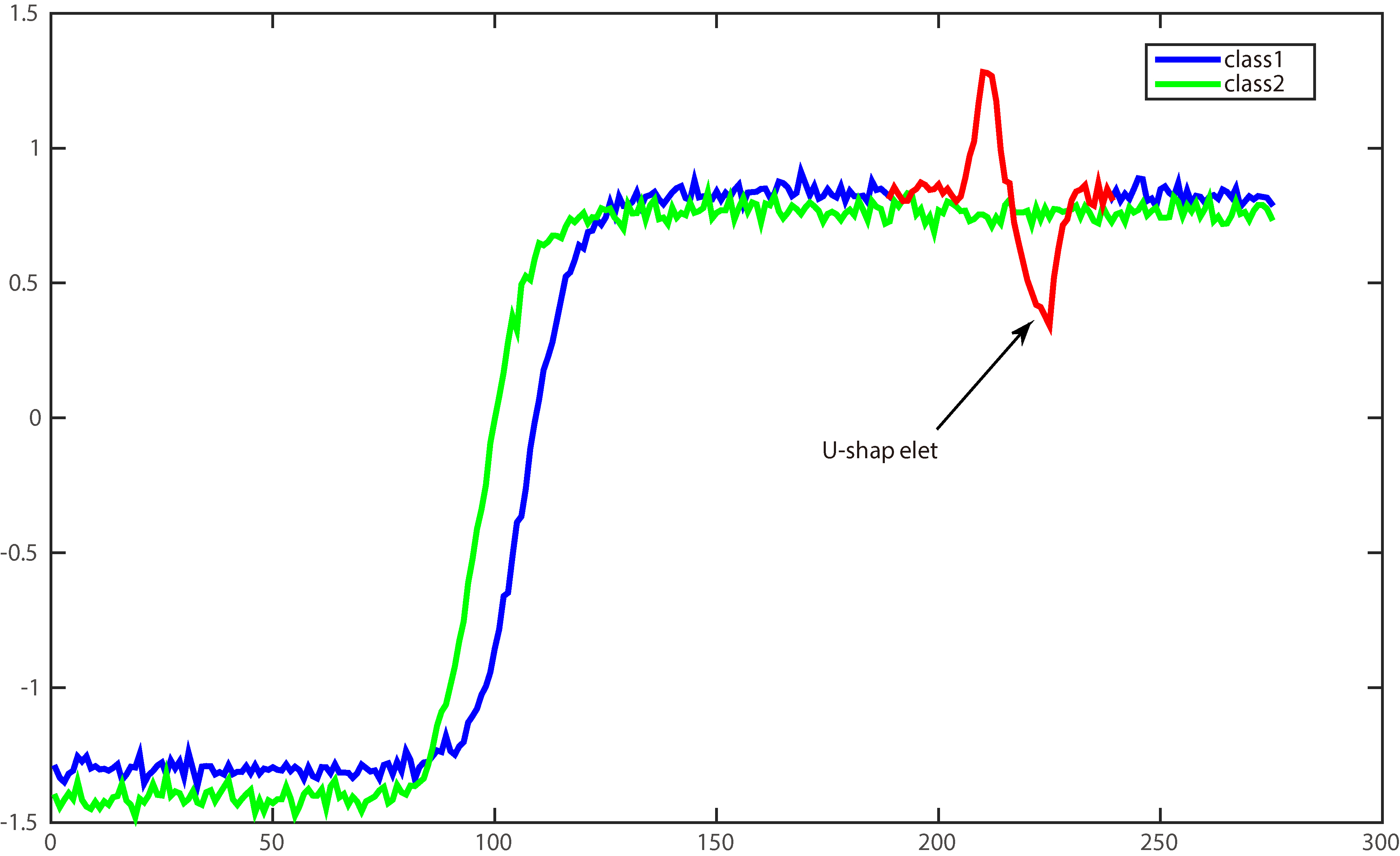

Moreover, the length of the time series can be unequal, which is not satisfied with most of the previous clustering works. These advantages have been confirmed by other researchers. However, the u-shapelet discovery process is very time-consuming. The straightforward way for finding u-shapelets is the exhaustive algorithm that generates all possible subsequences and examines these subsequences. The number of subsequences is liner in the number of time series in the dataset, and is quadratic in the length of the time series. These subsequences are u-shapelet candidates. In order to address the time-consuming problem, the Brute Force algorithm (the BF-algorithm for short) proposed by Zakaria et al. [15] only considers all possible subsequences of the first time series in the dataset, which makes the clustering result depend on the order of series in the dataset. If the first time series has few discriminative features, the result of time series clustering will be not good. Moreover, due to the fact that the u-shapelets extracted from a candidates subset, it is not guaranteed to achieve a comparable clustering result as the exhaustive search method.

An initial attempt at reducing the time consuming for discovering u-shapelets was published by Ulanova et al. [20]. The method (the SUSh-algorithm for short) is divided into two stages. Firstly, for all candidates of a given subsequence length, they use the Symbolic Aggregate approXimation (SAX) [13] technique to convert these continues real-valued candidates into a set of SAX words. Secondly, all SAX words are inserted into a table using a hash function, and a random projecting method [22] is used to filter out large numbers of candidates. The SUSh-algorithm has shown to be faster than the BF-algorithm. However, it has some disadvantages. Firstly, the method uses the hash table with random masking to identify similar subsequences which are really complicated. Secondly, the algorithm only extracts the u-shapelet candidates of a specific length. For a new dataset, we don’t have any prior knowledge about the appropriate length of u-shapelet.

1.2 Our contributions

In this paper, we inherit the merits and mitigate the limits of the above u-shapelets methods by introducing a Random Local Search algorithm (RLS-algorithm for short) that finds u-shapelets quickly with high-quality clustering result. The number of u-shapelet candidates examined with a random sampling way is only a small fraction of the exhaustive candidates. In the process of discovering u-shapelets, we introduce a local search strategy for refining the quality of u-shapelets. Our method exploits the fact that the discriminative subsequences are generally concentrated in local areas and are redundant.

Our contributions to this paper can be summarized as follows:

1.
We propose an effective method of randomly extracting the u-shapelet candidates. It can discover u-shapelets quickly which allow u-shapelet-based clustering method to be applied to large datasets.
2.
Our work can fast search the entire subsequences space after examining a tiny subset of all subsequences, which obtains a more excellent clustering result than the previous u-shapelets-based methods.
3.
We use the local search strategy to obtain an improved the clustering result which is close to the result of the exhaustive search method. It also mitigates the instability problem of the random results.
4.
A comparison between our method and two previous u-shapelet-based clustering algorithms is conducted.

The rest of the paper is organized as follows. Section 2 introduces the necessary background materials and definitions. In Section 3 we introduce our algorithm. Section 4 we present the experimental results of our algorithm. Finally, in Section 5 we give conclusions and directions for feature work.
2. Definitions and background

We firstly give the definition of time series:

.

A time series $T$ is a finite sequence of real-valued numbers $t_{i}$ on $i=1,2,\ldots,n$ . This number $n$ is the length of $T$ .

A dataset $D$ is a collection of $M$ such time series $\{T_{1},T_{2},\ldots,T_{M}\}$ . In this work, we are not focus on the entire time series, but on the part of time series that can best represent their classes.

.

Subsequences $S_{i,l}$ denote segments $t_{i},t_{i+1},\ldots,t_{i+l-1}$ of $T$ starting at position $i$ with length $l$ , for $1\leqslant i\leqslant n$ and $1\leqslant l\leqslant n-i+1$ .

For a time series of length $n$ , the number of all possible length subsequences are $\frac{n(n+1)}{2}$ . For a dataset of size $M$ with length $n$ , then there are a total of $M\times\frac{n(n+1)}{2}$ subsequences.

Even tiny differences in scale and offset can result in a great error, it is necessary to z-normalize [4] the time series before computing the distance [6] between time series. The z-normalization of a time series $T$ is defined as $T_{norm}=\frac{T-\mu}{\sigma}$ . Here, $\mu$ and $\sigma$ are the sample mean and standard deviation of $T$ . In this paper, different possible lengths of subsequence has to be considered. The Euclidean distance between short subsequences is expected to be shorter than the distance between long subsequences. Hence we take the length-normalized Euclidean distance[2] as the distance measure between two time series.

.

The normalized Euclidean distance between two time series $T_{1}$ , $T_{2}$ of length $n$ is calculated by the following formula:

$\textit{dist}(T_{1},T_{2})=\sqrt{\frac{1}{n}\sum_{i=1}^{n}(t_{1,i}-t_{2,i})^{2}}$ (1)

.

The distance between a time series $T$ of length $n$ and a subsequence $S$ of length $l$ is the minimum distance between $S$ and all the subsequences of $T$ that have the same length with $S$ , as shown in Eq. (2), where $1\leqslant l\leqslant n$ .

$\textit{sdist(S,T)}=\min_{1\leqslant j\leqslant n-l+1}\textit{dist}(S,T_{j,l})$ (2)

The minimum distance between a subsequence and a time series is the length-normalized Euclidean distance between the subsequence and the best matching subsequence of the time series. Figure 2 shows the idea.

Figure 2.

The minimum distance between a time series and a subsequence.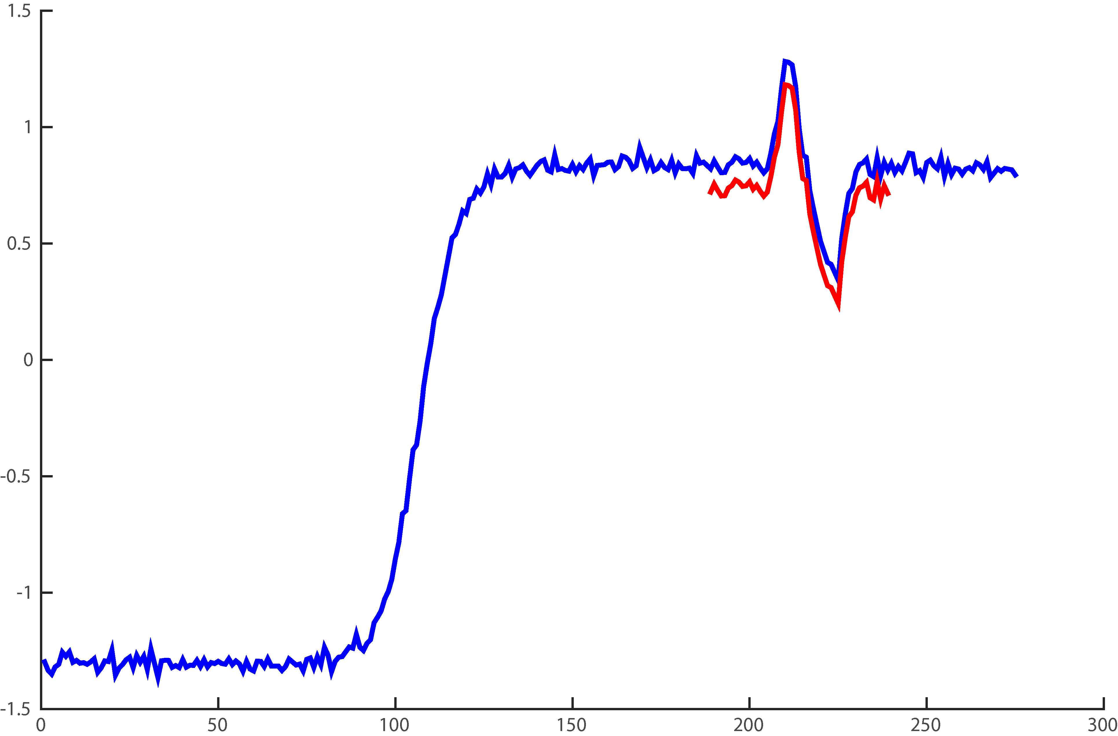

For each subsequence, we get a distance table which contains the sdist between the subsequence and all the time series in a dataset. The table is ordered increasingly by the sdist. Then the average distance between two adjacent distances is assigned as the split point. A greedy search algorithm is applied to separate the table into two subsets, i.e. the subset $D_{A}$ and $D_{B}$ .

.

An unsupervised-shapelet (u-shapelet) Ś is a subsequence that can divide a dataset $D$ into two groups, $D_{A}$ and $D_{B}$ . The sdist between Ś and any time series in group D ${}_{A}$ is much smaller than the sdist between Ś and any time series in D ${}_{B}$ .

A good u-shapelet is expected to split the dataset into two subsets that are as clearly distinction as possible. In the original method [15], the separation power of subsequence is evaluated by the following equation:

$gap=\mu_{B}-\sigma_{B}-(\mu_{A}+\sigma_{A})$ (3)

Here, $\mu_{A}$ and $\mu_{B}$ represent $\textit{mean}(\textit{sdist}(\acute{S},D_{A}))$ and $\textit{mean}(\textit{sdist}(\acute{S},D_{B}))$ respectively, while $\sigma_{A}$ and $\sigma_{B}$ represent $\textit{std}(\textit{sdist}(\acute{S},D_{A}))$ and $\textit{std}(\textit{sdist}(\acute{S},D_{B}))$ respectively. The larger the gap value is, the better separation effect it gets.

In the BF-algorithm, the u-shapelets are generated iteratively. First, all possible subsequences are extracted from the first series of dataset $D$ . Then for each subsequence, the gap value and the corresponding split point are computed. The subsequence with the maximal gap value is added to the u-shapelet set. Last they remove the time series whose distance is less than $\theta$ , a threshold $\theta$ is used in order to avoid removing time series whose distance is too close to split point. The threshold $\theta$ is defined by:

$\theta=\textit{mean}(\textit{sdist}(\acute{S},D_{A}))+\textit{std}(\textit{% sdist}(\acute{S},D_{A}))$ (4)

The process is repeated to generate the next u-shapelet in the rest of dataset. After generating a set of u-shapelets, the next step is to use them to cluster time series in $D$ .

.

The distance map[15] $D I S$ is a matrix containing the distance between all u-shapelets and all time series within $D$ . If there are $m$ u-shapelets and $M$ time series in $D$ , the distance map is shown in Eq. (5).

$\textit{DIS}=\left[\begin{matrix}\textit{sdist}(\acute{S}_{1},T_{1})&\textit{% sdist}(\acute{S}_{2},T_{1})&\cdots&\textit{sdist}(\acute{S}_{m},T_{1})\\ \textit{sdist}(\acute{S}_{1},T_{2})&\textit{sdist}(\acute{S}_{2},T_{2})&\cdots% &\textit{sdist}(\acute{S}_{m},T_{2})\\ \vdots&\vdots&\ddots&\vdots\\ \textit{sdist}(\acute{S}_{1},T_{M})&\textit{sdist}(\acute{S}_{2},T_{M})&\cdots% &\textit{sdist}(\acute{S}_{m},T_{M})\\ \end{matrix}\right]$ (5)

Then the distance map is used as the input to any off-the-shelve clustering algorithm such as k-means clustering [14], hierarchical clustering [18], etc. In BF-algorithm, a modified k-means algorithm is used for clustering through adding the distance vector to the distance map.

3. The random local search algorithm

In this section, we introduce our RLS-algorithm in detail.

3.1 A motivating observation

As a concrete example, we analyze the much-studied Trace dataset [31] which contains 200 time series of length 275 from four different classes. We extract a u-shapelet with the length of 60 from one time series of class 1. The Fig. 3 shows the u-shapelet and 19 subsequences around it.

Figure 3.

The neighbouring subsequences exhibits a similar pattern.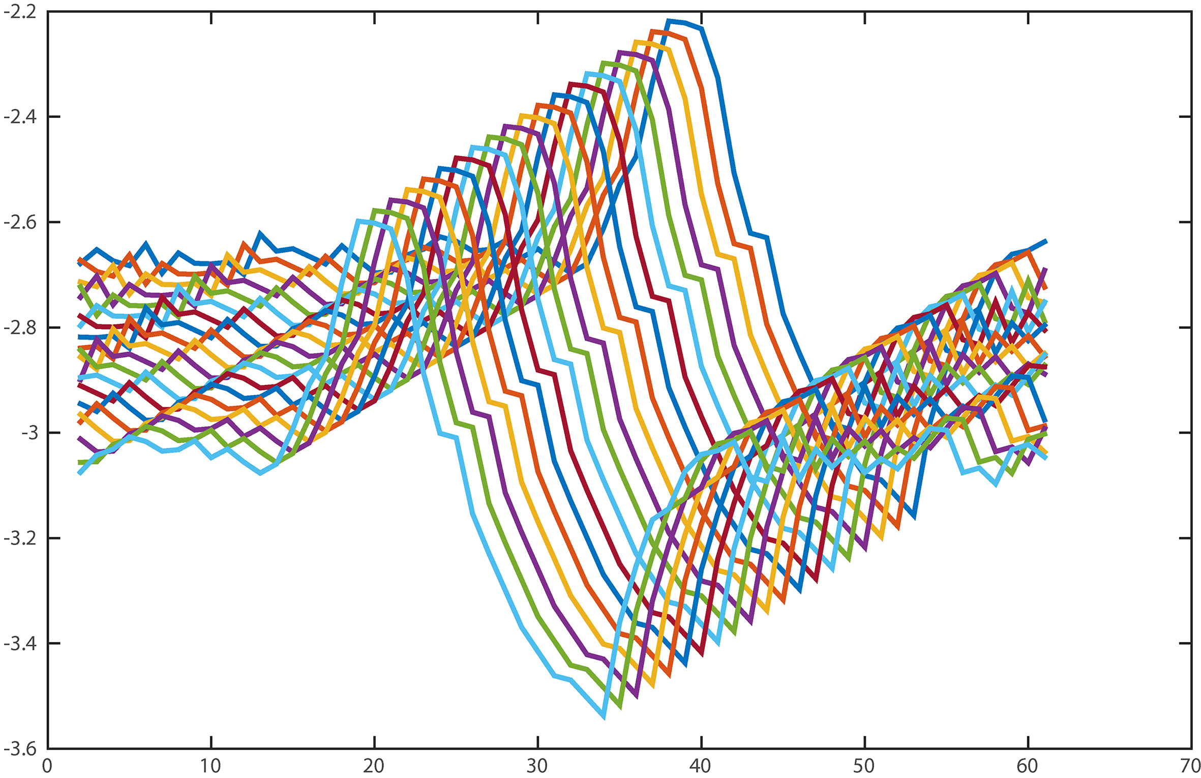

Clearly, the difference between two adjacent subsequences is extremely tiny. In many cases, the distances sdist between these subsequences and a new time series have no significant difference. Any subsequence from class 1 containing a similar pattern of the u-shapelet can be used to distinguish class 1 from other classes. Therefore, there is no need to exhaustively search the best u-shapelet for time series clustering, these subsequences that are similar to the pattern of the u-shapelet can be enough to obtain comparable results. We call these candidates as “good enough” u-shapelets. To understand how these “good enough” u-shapelets distribute in the candidates space, we do a simple test on the coffee dataset [31] which contains only 56 time series. Figure 4 shows the cumulative gap value of candidates of different lengths and different positions within the time series.

Figure 4.

The distribution of “good enough” candidates in candidates space.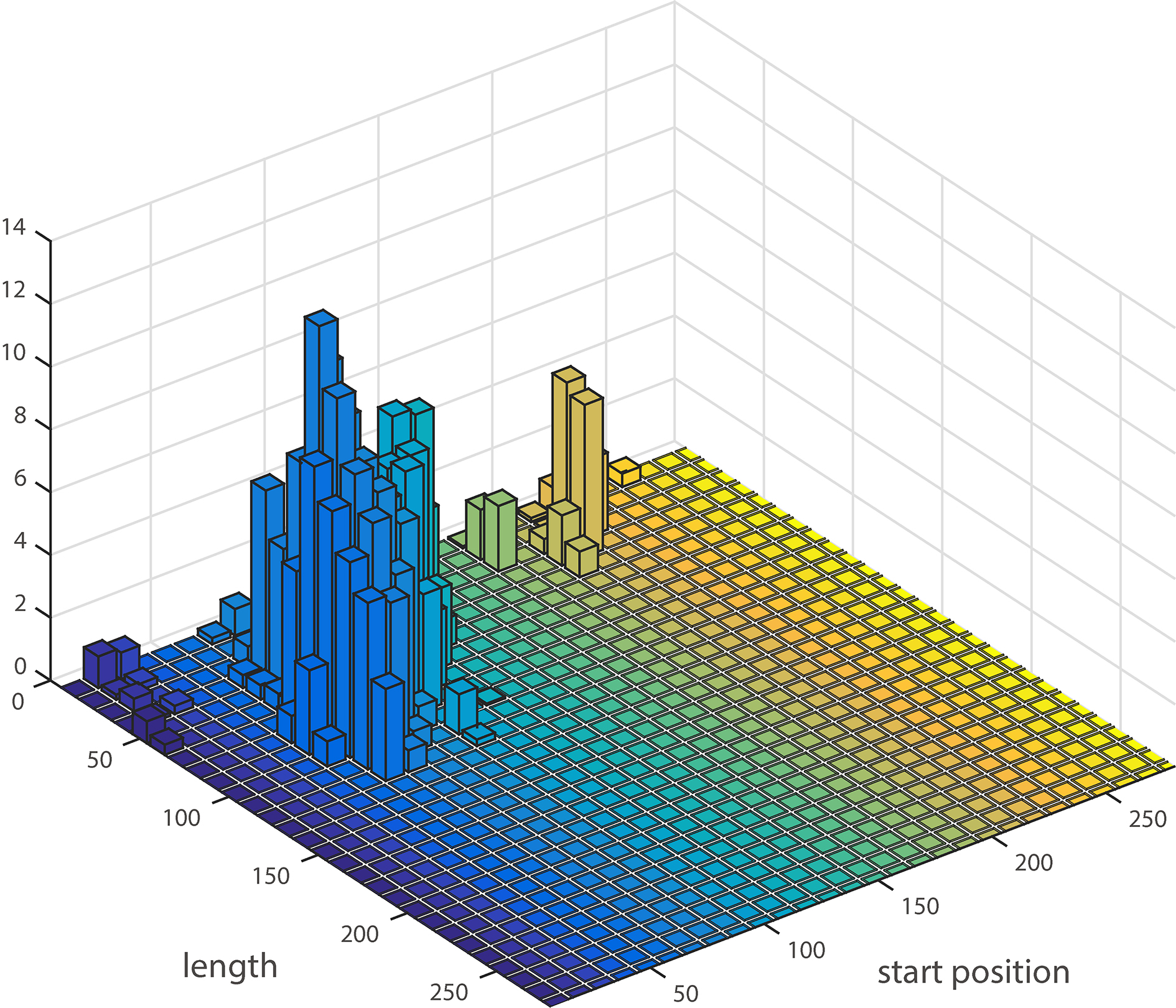

It is clear that these “good enough” u-shapelets from the same time series generally concentrate in local areas.

3.2 Random sampling

Sampling is the most effective approach to solve the scale of the input dataset, probably because it is easy to understand and implement [3]. UFS[21] employs random sampling to reduce the number of subsequences for time series classification. The experiment results show that a small fraction of sampling data is sufficient to achieve good classification results. Since we want to achieve “good enough” u-shapelets and we have no prior knowledge of where the informative candidates inside time series appear, we choose random sampling as our way of extracting candidates.

3.3 The random discovery process of u-shapelets

The u-shapelet discovery algorithm aims to obtain a set of u-shapelets which can be used to cluster time series, it’s the first step in our algorithm. The u-shapelet discovery process is carried out in an iterative way. At each iteration, the algorithm gets a u-shapelet with the maximal gap value from the u-shapelet candidates.

DiscoveryU-shapelet( $D$ , minlen, $m a x l e n$ , $r$ )[1] $D$ : dataset;maxlen,minlen: max and min length of u-shapelet; $r$ : number of u-shapelet candidates. $\acute{S}$ : set of u-shapelets $\acute{S}\leftarrow$ [] $count\leftarrow 1$ true $\textit{ush}\leftarrow$ FindU-shapelet( $D$ , minlen, maxlen, $r$ ) $\textit{dis}\leftarrow$ computeDistance( $D$ , ush) $D_{A}\leftarrow$ find( $\textit{dis}<\textit{ush}$ ( $s p$ )) // find all points left of the split point $s p$ $D_{B}\leftarrow D-D_{A}$ min(length( $D_{A}$ ), length( $D_{B}$ ))==1 break $\theta\leftarrow$ mean( $\textit{disD}_{A}$ )+std( $\textit{disD}_{A}$ ) $\acute{D}\leftarrow$ find( $\textit{dis}<\theta$ ) $D\leftarrow D-\acute{D}$ $\acute{S}$ (count) $\leftarrow\textit{ush}$ $\textit{count}\leftarrow\textit{count}+1$ return $\acute{S}$ FindU-shapelet( $D$ , minlen, maxlen, $r$ )[1] $D$ : dataset;maxlen,minlen: max and min length of u-shapelet; $r$ : number of u-shapelet candidates. ush: a u-shapelet $S\leftarrow$ [] $\textit{cnt}\leftarrow 1$ $\textit{times}\leftarrow r/(\textit{maxlen}-\textit{minlen}+1)$ $sl=\textit{minlen}$ to maxlen $t=1$ to round(times) $ts\leftarrow U(1,M)$ $i\leftarrow U(1,n-sl+1)$ $s_{ts,sl,i}\leftarrow D(ts,i:i+sl-1)$ $[\textit{gap,sp}]\leftarrow$ computeGap $(s_{ts,sl,i},D)$ $\textit{S(cnt) }\leftarrow{(ts,sl,i,gap,sp)}$ $cnt\leftarrow cnt+1$ $S\leftarrow$ sortByGap $(S)$ $k\leftarrow r/10$ $S_{k}\leftarrow$ TopkCandidates $(S,k)$ $S_{k}\leftarrow$ LocalSearch $(D,S_{k})$ $\textit{index}\leftarrow$ maxGap $(S_{k})$ $\textit{ush}\leftarrow S_{k}(\textit{index})$ return ush

The Algorithm 3.3 provides the basic framework for discovering u-shapelets. The input has four parameters namely $D$ , $r$ , maxlen, minlen. $D$ : the dataset of time series; $r$ : the number of candidates to examine; $m a x l e n$ : the max length of the candidate; minlen: the min length of the candidate. Line 4 executes the random extraction process that is a key part of finding a u-shapelet. In line 5, the distances between the current u-shapelet ush and all time series within $D$ are computed and stored in a distance vector dis. In lines 6–7, the u-shapelet ush split dataset $D$ into two subsets, the $D_{A}$ set and the $D_{B}$ set. Line 8 gives the condition for the u-shapelet discovery process termination. In lines 11–13, we update the $D$ by removing time series that are similar to current u-shapelet. Finally, the set of u-shapelets $\acute{S}$ is returned.

The Algorithm 3.3 is a subroutine in line 4 of Algorithm 3.3 to find a u-shapelet. The parameters are the same as Algorithm 3.3.

We first randomly extract $r$ subsequences from the exhaustive subsequences space as the u-shapelet candidates. Since every subsequence has the same probability of being extracted, the random function assumes it has a uniform distribution in candidates space. In line 1, the set of u-shapelet candidates $S$ is initialized empty. In line 3, the number of candidates to be extracted of every length is computed. In the nested for loop of lines 4–13, $r$ subsequences of different length are extracted uniformly at random, forming a u-shapelet candidates set $S$ . For each subsequence of a specific length $s l$ , we randomly select a time series $t s$ from the dataset $D$ , and randomly determine a start position $i$ . Once determining the three parameters, a subsequence $s_{ts,sl,i}$ can be extracted from the dataset $D$ . The gap value gap and corresponding split distance $s p$ of the current candidate are calculated by the computeGap algorithm, please refer to [15] for more details. Note that we extract one candidate in each iteration until the number of iteration is reached. The main reason for this is to save memory space. All the candidates’ information is stored in the set $S$ . In line 14, the u-shapelet candidates in $S$ are sorted in a descending order by their gap values. In lines 15–16, instead of choosing the initial $k$ candidates arbitrarily, we get the top-k candidates for further searching, where $k$ is set to $r/10$ . In line 17, to refine the quality of the $k$ candidates, we introduce the local search strategy. Next subsection we explain the local search process in detail. Once the local search process competes, the candidate with the maximal gap value as a u-shapelet is returned.

3.4 The local search strategy

In Subsection 3.1, we have analyzed that the high-quality of u-shapelet candidates is usually concentrated in local areas. The gap value of adjacent subsequences roughly first increases then decreases, as shown in Fig. 5. Starting with the top-k candidates, that is to say, we first select $k$ good initial value for the local search method. The local search process aims to iteratively check if swapping the current candidate with one of the neighborhood subsequences would improve the gap value, and makes the local exchange if it is profitable.

A neighborhood is the solution subspace of the current solution which defines the available moves for generating a new solution [11]. In this paper, we define a neighborhood by creating a circular plane that places the current candidate as its center. For a given candidate $s$ starting at position pos with length slen, we define the neighborhood $N$ as follows:

$N=\{s_{j}:\mid s_{j}-s\mid\leqslant R\}$ (6)

Here $R$ is the radius of the neighborhood, and $\mid s_{j}-s\mid$ is defined by:

$d(x,y)=\sqrt{(\textit{pos}_{x}-\textit{pos}_{y})^{2}+(\textit{slen}_{x}-% \textit{slen}_{y})^{2}}$ (7)

We treat the current candidate as a 2-dimensional point, where the first dimension represents the start position pos and the second dimension represents the length slen. Any subsequence from the same series satisfying the condition indicated in Eq. (6) becomes an element of the neighborhood $N$ . The local search procedure is shown in Algorithm 3.4. LocalSearch( $D$ , $S_{k}$ )[1] $D$ : dataset; $S_{k}$ : the $k$ candidates set; $S_{k}$ : the $k$ local optimal candidates set $\textit{cnt}=1$ to $k$ true $\textit{gap}\leftarrow$ the gap value of $S_{k}$ (cnt) $N\leftarrow$ CreateNeighborhood( $S_{k}$ (cnt)) each subsequence $s$ in $N$ $[\textit{gap,sp}]\leftarrow$ computeGap $(s,D)$ $\textit{maxgap}\leftarrow$ max(N(gap)) // select the largest gap value in the neighborhood $N$ $\textit{maxgap}>\textit{gap}$ $S_{k}$ (cnt) $\leftarrow$ $N$ (maxgap) // a new better u-shapelet candidate is found break return $S_{k}$

Figure 5.

The gap value of the 20 adjacent subsequences from the same series roughly first increases then decreases, there is a maximum gap value.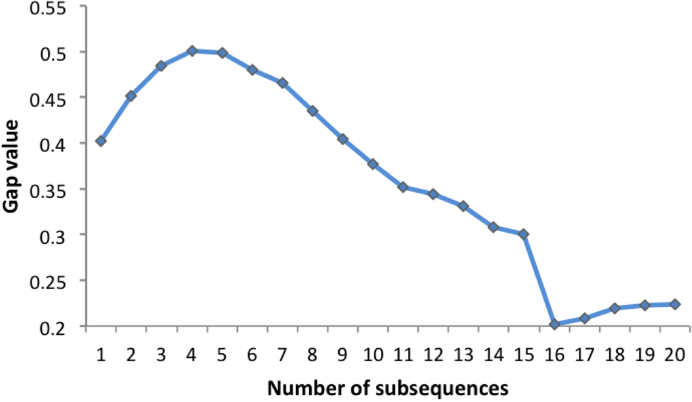

For each candidate, we first get the gap value of the current u-shapelet candidate in line 3. In line 4, a neighborhood $N$ of the current candidate is created. In lines 5–7, we compute the gap value of the subsequences within the neighborhood $N$ . If the maximal gap value of these neighborhood subsequences is larger than that of the current candidate, the subsequence with maximal gap value to replace the current candidate. The procedure stops after the current search converges to a local optimal solution. Based on the new current candidate, we perform the above steps, the search process terminates as soon as the stopping criterion is fulfilled. Finally, the $k$ local optimal candidates are returned. We demonstrate that the local search strategy can make the clustering result tends to more accurate and stable by iterative improving the quality of candidates.

Table 1

Information of datasets used in our experiment

Dataset	Size	Length	Classes
Beef	60	470	5
Birds	177	500	2
CBF	930	128	3
Coffee	56	286	2
ECGFiveDays	884	136	2
ECG_PVC	166	144–698	2
ECG_APB	164	140–699	2
ECG_RT	126	146–700	2
FaceAll	2250	131	14
FaceFour	112	350	4
FacesUCR	2250	131	14
FISH	350	463	7
GunPoint	200	150	2
ItalyPowerDemand	1096	24	2
Lighting2	121	637	2
Lighting7	143	319	7
Mallat	2400	1024	8
MedicalImages	1141	99	10
OSULeaf	442	427	6
PAMAP	345	500	7
Plane	210	144	7
StartLightCurves	9236	1024	3
Swedishleaf	1125	125	15
Symbols	1020	398	6
Syn_Control	600	60	6
Trace	200	275	4
TwoLeadECG	1162	82	2

4. Experimental evaluation

In this section, we describe the results of our experimental evaluation. There are two criteria to evaluate the efficiency of our method. The first one is the quality of time series clustering result. The second one is the runtime of the whole process of u-shapelet discovery. A popular quality measure for evaluation of time series clustering is the Rand index (RI) [30] measures the correctness the sorting of elements into clusters. The RI is a number lies between 0 and 1, where it is close to 1 means a perfect clustering result. Additionally, the standard deviation of the clustering results is used to measure the stability of our method.

We conduct our experiments through two parts. In the first part, we determine the parameters of our algorithm, the two length parameters minlen and maxlen, and the best number of candidates to sample $r$ . In the second part, in terms of the parameters determined on first part, we compare our RLS-algorithm with other two u-shapelets-based clustering algorithms. Additionally, we apply our algorithm on some large datasets to prove that the RLS-algorithm is useful on large datasets.

4.1 Datasets

The experiment was carried out on 27 datasets from various domains such as speech recognition, activity recognition, medicine, image classification and several more. The datasets of Birds, ECG_PVC, ECG_APB, ECG_RT and PAMAP can be obtained form the paper [20]. The rest of the 22 datasets can be downloaded from the UCR Time Series archives [31] which is used commonly for time series classification and clustering. All of these datasets from the UCR Time Series archives have been split into 2 subsets: training and test sets. In our work, we use the mixed dataset, which consists of both training and test sets. Note that all the previous time series classification methods are experimented on small training set to discover shapelets.

Table 1 summaries the datasets we used which consist of both synthetic and real-world time series datasets. The dataset size ranges from 56 to 9236, the number of classes varies from 2 to 15 and the length of the time series varies from 24 to 1024. We use the largest dataset of the UCR datasets, StarLightingCurves, which contains 9236 time series of length 1024. In addition, many of the datasets contain noise or missing data such as CBF, Mallat, Syn_Control, etc. There are also 3 datasets contain time series with unequal length namely ECG_PVC, ECG_APB and ECG_RT. It proves the u-shapelets-based methods can be applied to the time series clustering with different length.

4.2 Determination of u-shapelet length

The process of u-shapelet discovery needs to set two parameters of length: minlen and maxlen. The two parameters determine the range of u-shapelet length, which control the scope of the discovery and help make the discovery process more efficient. However, it will prevent those informative subsequences from being selected if the parameters are setting inappropriate. If the length of u-shapelets is too short, the discriminant information contained is too small to represent the characteristics of the time series. If the length of the u-shapelet is too long, which is actually no difference compared with whole time-series. The advantages of accurate and interpretable of the u-shapelet technique are not reflected. We don’t have any prior knowledge about the appropriate u-shapelet length. So followed [12], we set the minimum length of u-shapelet to $m/11$ and the maximum length to $m/2$ , where the $m$ is the minimum length of time series in a dataset.

4.3 Determination of r

The process also requires adjusting the parameter $r$ that represents the number of candidates needed to find a u-shapelet. In order to explain how the $r$ value influences the effectiveness of time series clustering result, we do a test on 4 representative datasets with the varying $r$ value. The size of the datasets varies from 200 to 2250. The $r$ is set to 10, 50, 100, 200, 500, 1000, 2000, 5000, 10000. For each dataset, we execute the test 10 times, and the average result of every point is summarized in Figs 6 and 7. Note that all of the experiments in this paper are performed 10 times.

Figure 6.

Clustering result varying with 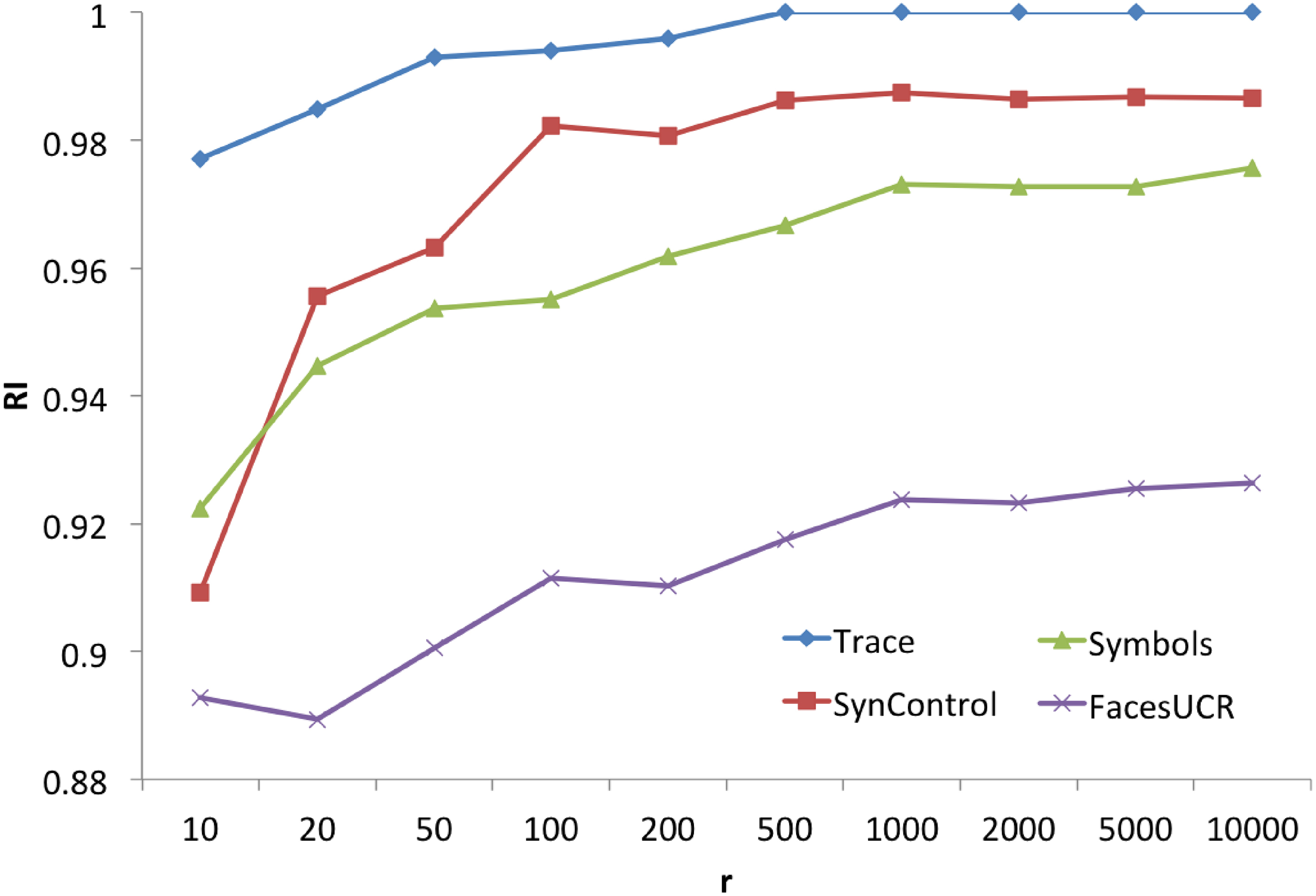$r$ .

Figure 7.

Runtime result varying with 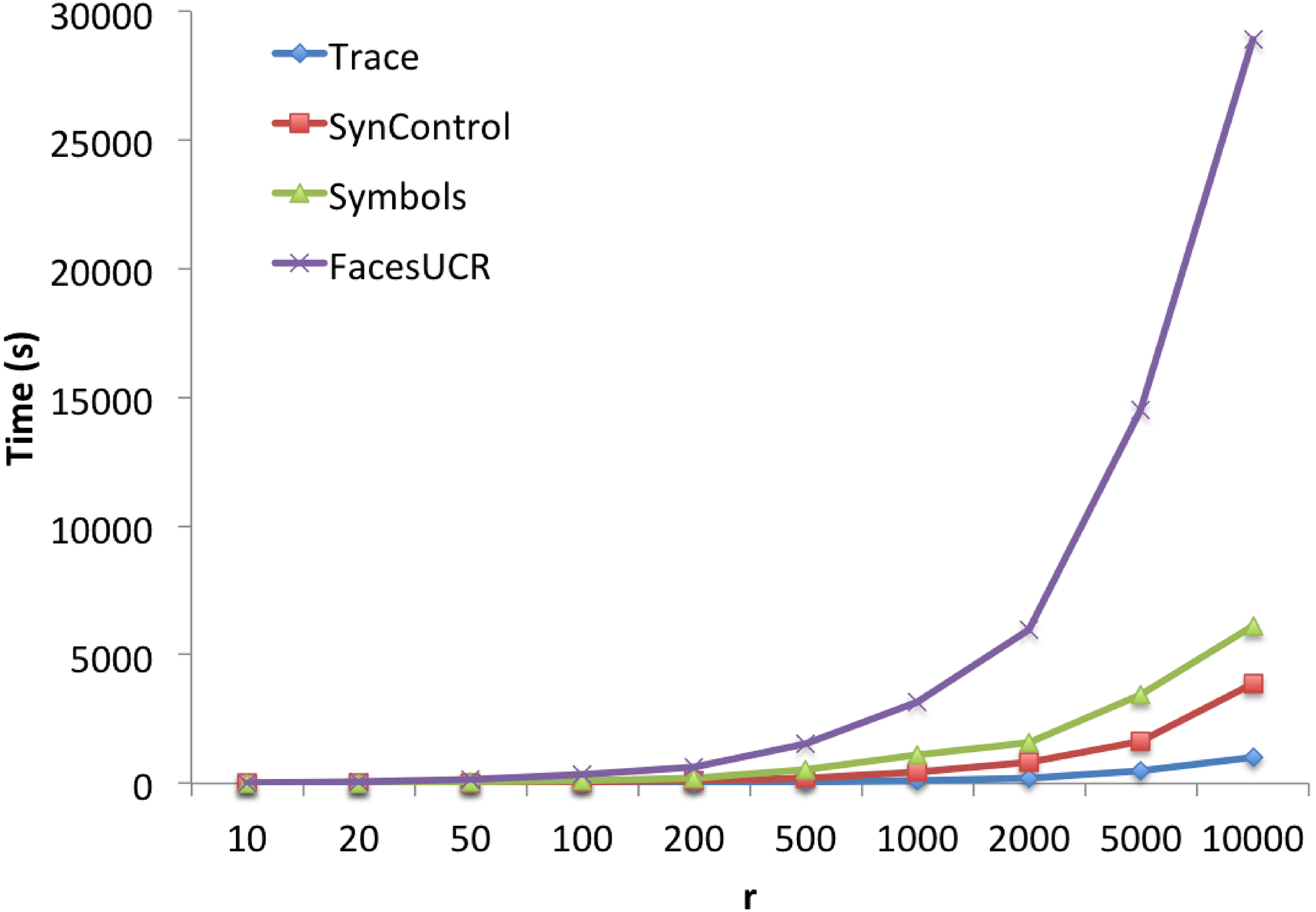$r$ .

Figure 6 shows the accuracy of time series clustering. We can clearly see that the initial RI value of our RLS-algorithm remains close to the final result. This probably thanks to the randomization, a “good enough” u-shapelet is quickly obtained. With the increasing of $r$ value, average clustering result first increases then becomes stable when $r$ is 1,000. The runtime results of our RLS-algorithm against different $r$ value on 4 datasets are shown in Fig. 7. The observation is that RLS-algorithm’s runtime is approximately linear to the size of $r$ . In the following of the paper, we will set $r=$ 1,000. We can apply the probability theory to estimate the confidence of the random sampling method. Assuming that the probability of obtaining a “good enough” u-shapelet is 0.01, then after extracting 1000 subsequences, The probability that any subsequence can fall in the high gap value area is $1-0.99^{1000}=$ 0.999956829.

4.4 Effectiveness of our method

4.4.1 Compared with the BF-algorithm

To evaluate the effectiveness of u-shapelets generated by our algorithm, we compare the clustering result and execution time of our RLS-algorithm with the BF-algorithm which is the first article clustering time series with u-shapelets. The comparison is done on 17 small datasets from the UCR Time Series archives as the BF-algorithm on a large size dataset or on a dataset with a large time series length for u-shapelet discovery is extremely time-consuming. Table 2 represents the average results of each dataset. In particular, all experiments are done in the same environment and on the same input datasets, and the results of the BF-algorithm are reproduced with code available online. So we can be sure that the improvement is valid.

Table 2
Comparison between RLS-algorithm and the BF-algorithm

Dataset	R			Runtime (sec)
	BF-algorithm	RLS-algorithm	K-means	BF-algorithm	RLS-algorithm	Speedup
Trace	1.0000	1.0000	0.7495	3898.1843	106.6823	36.5401
SynControl	0.8992	0.9875	0.8705	622.6931	402.6953	1.5463
GunPoint	0.7437	0.7587	0.4975	846.9162	124.4983	6.8026
CBF	0.7787	0.9267	0.6092	3180.5103	351.7007	9.043
Coffee	0.9299	0.9823	0.8052	989.8250	26.8873	36.8138
ECGFiveDays	0.5021	0.9363	0.5001	4353.4728	496.8726	8.7617
FaceFour	0.7735	1.0000	0.7233	7077.5125	125.5176	61.4058
Lighting2	0.5083	0.5632	0.5172	44885.0798	136.4867	328.8605
Fish	0.8480	0.8832	0.7792	44493.7842	325.7482	136.5895
Lighting7	0.7195	0.8356	0.8204	12278.6967	153.9751	79.7447
OsuLeaf	0.8072	0.8353	0.7508	21495.2540	397.3167	54.1011
SwedishLeaf	0.9257	0.9295	0.8813	4412.1414	336.3055	13.1194
TwoLeadECG	0.5081	0.8678	0.5021	1424.9556	251.9761	4.0484
MedicalImages	0.6743	0.6931	0.6505	1712.8940	375.4810	4.5619
ItalyPowerDemand	0.8491	0.8653	0.5032	189.4807	179.1983	1.0574
Beef	0.6712	0.7049	0.6441	5234.7328	56.1380	93.2476
Plane	0.9973	0.9945	0.9502	1086.7754	153.2173	7.0930

According to the results of Table 2, we observe that our RLS-algorithm clearly outperforms the BF-algorithm. In the third column of Table 2, the results by using the k-means algorithm on the whole time series are presented as a reference. In terms of the runtime, the time required to discover u-shapelets of our RLS-algorithm and that of the BF-algorithm are recorded in the 5–6 columns of Table 2. The last column lists the speedup factors of our method over the BF-algorithm, the greatest speedup we obtain on these 17 small datasets is 328 times, and we gain an average speedup exceeding 52 times. For the sake of clarity, we display the clustering results in Fig. 8. We also found that the speedup effect on some datasets is significant, while that of on some datasets is not satisfactory. The main reason is that the BF-algorithm only considers all possible subsequences of the first time series in a dataset, which makes the clustering result depend on the order of series in a dataset. If the length of the time series is short, the runtime of BF-algorithm is acceptable, but the clustering results may not be so ideal. In general, it is clearly that our method obtains more excellent results than the BF-algorithm.

Figure 8.

The clustering result comparison with BF-algorithm.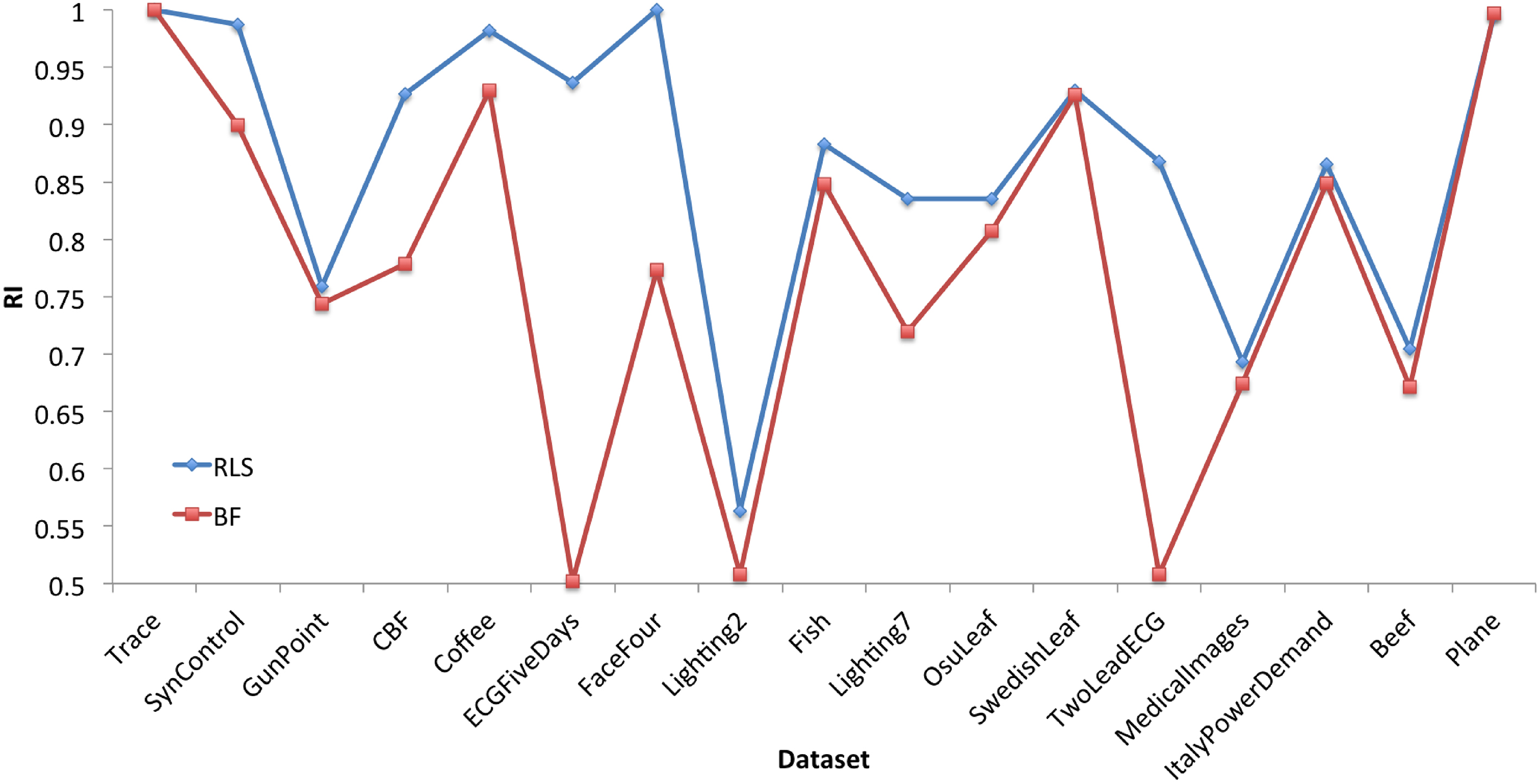

To further confirms that the effectiveness of the local search strategy, we present a comparison of our RLS-algorithm versus the simple random algorithm without local search process on the above 17 datasets. The means and standard deviations of the two methods are presented in Figs 9 and 10 respectively.

Figure 9.

The average clustering results comparison between RLS-algorithm and the simple Random algorithm on 17 datasets.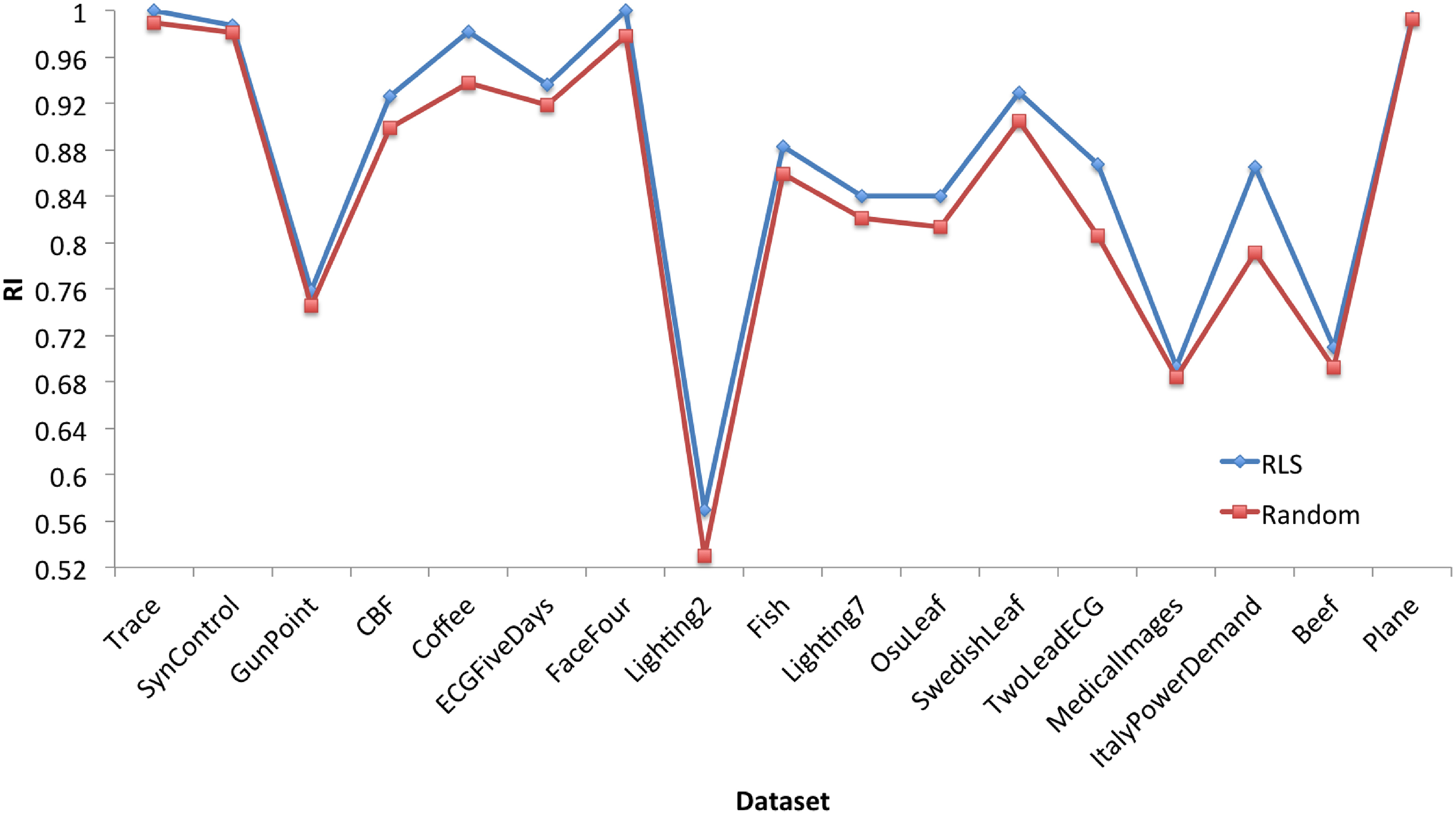

According to Figs 9 and 10, we conclude that our RLS-algorithm achieves more accurate clustering result than the random algorithm, while the standard deviations of our method are lower than that of the random method. It illustrates that the local search method gives an improvement in the clustering result, which makes the clustering results more better and stable.

4.4.2 Compared with the SUSh-algorithm

In this subsection, we compare clustering accuracy and runtime of our RLS-algorithm with the SUSh-algorithm which is the current state of the art and is faster than the BF-algorithm. Since the SUSh-algorithm examines subsequences of a given length, and the SUSh-algorithm did not give the appropriate length for every dataset, the suitable length for u-shapelets is a difficult question to answer. To ensure a fair comparison, we re-implement the SUSh-algorithm with all possible lengths of u-shapelets, which requires a lot of work. Because the SUSh-algorithm uses a random projecting method to filter out large numbers of candidates, the result of each time is non-deterministic. The experiment results of the SUSh-algorithm in this paper are also performed 10 times. We compare the SUSh-algorithm with the proposed RLS-algorithm on all the datasets used in [20], except for the AMPds dataset that we did not get.

Table 3 records the Rand index of the two algorithms. It is clearly that our method achieves the same or even surpasses the quality of clustering as the SUSh-algorithm. The execution time of RLS-algorithm and that of the SUSh-algorithm are presented in Table 4. It illustrates that the runtime of RLS-algorithm is approximately same as that of the SUSh-algorithm. In summary, our method produces higher clustering quality than the SUSh-algorithm in the same time order of magnitude.

Table 3
Rand Index of RLS-algorithm and the SUSh-algorithm

Dataset	SUSh-algorithm	RLS-algorithm	K-means
Trace	1.0000	1.0000	0.7495
PAMAP	0.9267	0.9303	0.7541
Birds	0.9664	0.9798	0.7726
ECG_PVC	0.9760	0.9760	Not defined
ECG_APB	0.9685	1.0000	Not defined
ECG_RT	0.9660	0.9903	Not defined

Figure 10.

The standard deviations of RLS-algorithm and that of Random algorithm on 17 datasets.

Table 4

Execution time of the RLS-algorithm and the SUSh-algorithm

Dataset	SUSh-algorithm (min)	RLS-algorithm (min)
Trace	2.3501	1.7780
PAMAP	10.2266	7.8054
Birds	1.6228	1.7421
ECG_PVC	0.9900	1.5577
ECG_APB	0.4002	1.0472
ECG_RT	0.5904	1.1148

4.4.3 Evaluation on large datesets

This subsection will demonstrate that our method can be applied to large datasets. Thanks to the time reduction obtained with our RLS-algorithm, it is possible to allow large datasets to be analyzed in a reasonable time. We consider 5 datasets which size are larger than 1000 and the length of time series is quite long, the average clustering results are presented in Table 5.

Table 5
Results of the RLS-algorithm on 5 large datasets

Dataset	RI		Runtime (sec)
	RLS-algorithm	K-means
FaceAll	0.9264	0.8784	3467.9338
FacesUCR	0.9238	0.8878	3235.6344
Mallat	0.9898	0.9542	6621.3460
StarLightCurves	0.7880	0.7704	22934.8340
Symblos	0.9731	0.8994	1128.5714

As shown in Table 5, our u-shapelet discovery method is effective on the large dataset. Moreover, the time consumption of all datasets is reasonable, which has shown that RLS-algorihtm is especially helpful to solve the time-consuming problem of u-shapelet discovery on large datasets.

5. Conclusions and future work

In this paper, we analyze the natural feature of time series subsequences and propose a Random Local Search algorithm to reduce the time complexity of the u-shapelet discovery. By using the random sampling technique, we reduce the size of the u-shapelet candidates set with a modification of the discovery process. By using the local search strategy, we improve the quality of the clustering result. Experiments indicate that our algorithm outperforms recently proposed approaches on both synthetic and real dataset in the time series clustering. Moreover, we also show the utility of our algorithm on large datasets.

Further work includes attempts to use methods of local search to further refine the quality of u-shapelets, as it may be more effective for improving the quality of u-shapelets. another future direction of work could consist in sampling subsequences from these feature points, instead of sampled randomly or uniformly.

Footnotes

Acknowledgments

The first author thanks Jesin Zakaria who provided the source code in .

References

Kotsifakos

Athitsos

and Papapetrou

, Query-sensitive distance measure selection for time series nearest neighbor classification, Intelligent Data Analysis 20(1) (2016), 5–27.

Mueen

Keogh

and Young

, Logical-shapelets: An expressive primitive for time series classification, in: Proceedings of the 17th ACM SIGKDD Internatinal Conference on Knowledge Discovery and Data Mining, 2011, 1154–1162.

Stuart

, Basic ideas of scientific sampling, Journal of the Operational Research Society 28(3) (1977), 612–612.

Chen

and Keogh

, Time series classification under more realistic assumptions, in: Proceedings of the 2013 SIAM International Conference on Data Mining, 2013, pp. 578–586.

Berndt

D.J.

and Clifford

, Using dynamic time warping to find patterns in time series, International Conference on Knowledge Discovery and Data Mining 10(16) (1994), 359–370.

Keogh

and Kasetty

, On the need for time series data mining benchmarks: a survey and empirical demonstration, Data Mining and Knowledge Discovery 7(4) (2003), 349–371.

Ruiz

E.J.

Hristidis

and Castillo

Gionis

, Correlating financial time series with micro-blogging activity, in: Proceedings of the fifth ACM International Conference on Web Search and Data Mining, 2012, 513–522.

Iglesias

and Kastner

, Analysis of similarity measures in times series clustering for the discovery of building energy patterns, Energies 6(2) (2013), 579–597.

Box

G.E.P.

and Jenkins

, Time series analysis, forecasting and control, in: Holden-Day, Incorporated, 1990.

10.

Ding

Trajcevski

Scheuermann

Wang

and Keogh

, Querying and ming of time series data: experimental comparison of representations and distance measures, Proceedings of the VLDB Endowment 1(2) (2008), 1542–1552.

11.

Ishibuchi

and Murata

, An multi-objective genetic local search algorithm and its application to flowshop scheuling, IEEE Transactions on Systems, Man, and Cybernetics, Part C (Applications and Reviews) 28(3) (1998), 392–403.

12.

Hills

Lines

and Baranauskas

, Classification of time series by shapelet transformation, Data Mining and Knowledge Discovery 28(4) (2014), 851–881.

13.

Lin

Keogh

Lonardi

and Chiu

, A symbolic representation of time series, with implications for streaming algorithm, in: Proceedings of the 8th ACM SIGMOD Workshop on Research issues in Data Mining and Knowledge Discovery, 2003, pp. 2–11.

14.

MacQueen

, Some methods for classification and analysis of multivariate observation, Proceedings of the fifth Berkeley symposium Mathematical Statist Probability 1(14) (1967), 281–297.

15.

Zakaria

Mueen

and Keogh

, Clustering time series using unsupervised-shapelets, in: Proceedings of the 2012 IEEE 12th International Conference on Data Mining, 2012, 785–794.

16.

and Keogh

, Time series shapelets: A new primitive for data mining, in: Proceedings of the 15th ACM SIGKDD Internatinal Conference on Knowledge Discovery and Data Mining ACM, 2009, pp. 947–956.

17.

and Prakash

, Time Series Clustering: complex is simpler!, in: Proceedings of the 28th International Conference on Machine Learning, 2011, pp. 185–192.

18.

Kaufman

Rousseeuw

P.J.

and Corporation

, Finding groups in data: an introduction to cluster analysis, John Wiley & Sons, 344 (2009).

19.

and Keogh

E.J.

, Time series shapelets: A novel technique that allows accurate, interpretable and fast classification, Data Mining Knowledge Discovery 22(1) (2011), 149–182.

20.

Ulanova

Begum

and Keogh

, Scalable clustering of time series with u-shaplets, in: Proceedings of the 2015 SIAM International Conference on Data Mining, 2015, pp. 900–908.

21.

Wistuba

Grabocka

and Schmidtthieme

, Ultra-Fast shapelets for time series classification, in: Preprint submitted to Journal of Data & Knowledge Engineering, 2015.

22.

Tompa

and Buhler

, Findings motifs using random projections, Journal of Computational Biology 9(2) (2002), 225–242.

23.

Subhani

Rueda

Ngom

and Burden

C.J.

, Multiple gene expression profile alignment for microarray time-series data clustering, Bioinformatics 26(18) (2010), 2281–2288.

24.

Zhu

Bastita

Rakthanmanon

and Keogh

, A novel approximation to dynamic time warping allows anytime clustering of massive time series datasets, in: Proceedings of the 2012 SIAM International Conference on Data Mining, 2012, pp. 999–1010.

25.

Kohavi

, A study of cross-validation and bootstrap for accuracy estimation and model selection, in: Proceedings of the 14th International Joint Conference on Artificial Intelligence (2) (1995), pp. 1137–1145.

26.

Hirano

and Tsumoto

, Cluster analysis of time series medical data based on the trajectory representantion and multiscale comparison techniques, in: International Conference on Data Mining IEEE Computer Society, 2006, pp. 896–901.

27.

Aghabozorgi

Shirkhorshidi

A.S.

and Yang Wah

, Time-series clustering-a decade review, Information Systems 53 (2015), 16–38.

28.

Salvador

and Chan

, Toward accurate dynamic time warping in linear time and space, Intelligent Data Analysis 11(5) (2007), 561–580.

29.

Rakthanmanon

and Keogh

, Fast shapelets: A scalable algorithm for discovering time series shapelets, in: Proceedings of the Thirteenth SIAM Conferences on Data Mining. Society for Industrial and Applied Mathematics, 2013, pp. 668–676.

30.

Rand

W.M.

, Objective criteria for the evaluation of clustering methods, Journal of the American Statistical Association 66(336) (1971), 846–850.

31.

Chen

Y.P.

Eamonn

Begum

Bagnall

Mueen

and Batista

, The UCR time series classfication/clustering archive, Homepage: http://www.cs.ucr.edu/∼eamonn/time_series_data/, 2015.

RLS : An efficient time series clustering method based on u-shapelets

Abstract

Keywords

1. Introduction

1.1 Related work

.

.

.

.

.

.

3.1 A motivating observation

3.3 The random discovery process of u-shapelets

3.4 The local search strategy

4.1 Datasets

4.2 Determination of u-shapelet length

4.3 Determination of r

4.4.1 Compared with the BF-algorithm

Table 2 Comparison between RLS-algorithm and the BF-algorithm

Table 3 Rand Index of RLS-algorithm and the SUSh-algorithm

Table 5 Results of the RLS-algorithm on 5 large datasets

Footnotes

Acknowledgments

References

Table 2
Comparison between RLS-algorithm and the BF-algorithm

Table 3
Rand Index of RLS-algorithm and the SUSh-algorithm

Table 5
Results of the RLS-algorithm on 5 large datasets