If we endow an intelligent system with fuzzy logic, we hope that it can deal with fuzzy data, including the clustering of fuzzy data. This paper proposes a fuzzy mixed data clustering algorithm by fast search and find of density peaks (FMTD-CFSFDP), which is a development of the CFSFDP clustering algorithm. The proposed algorithm is a kind of density-based clustering method established using fuzzy sets for fuzzy mixed data. Mathematical definitions for fuzzy mixed data are presented. Combined with the definition of traditional fuzzy Euclidean distance, we defined an improved Euclidean distance for both continuous and discrete fuzzy sets with smaller error. On this basis, the weight between continuous and discrete indicators is introduced for establishing the global difference for fuzzy mixed data. Referring to the clustering procedures of the CFSFDP algorithm, a Gaussian Kernel function for fuzzy samples is calculated and the clustering procedures of our proposed algorithm are described in detail. Furthermore, four different sets of random simulations are performed, which illustrates the feasibility of the proposed algorithm.
Clustering analysis refers to the process of dividing data objects or observed objects into various subsets in accordance with certain standards such as distance or density. Each subset represents a cluster. Clustering is a kind of generalized system, as it has three key elements: input, processing and output. When clustering, we input some objects to be clustered (sample sets or datasets), the clustering algorithm will process these objects according to certain standards (e.g., a mathematical model), and output different clusters which contains different objects.
Clustering analysis is a kind of unsupervised learning process, with the aim of making clusters that contain similar objects within a cluster with these being dissimilar to other objects in other clusters [1, 22]. Currently, clustering analysis has been widely applied in many fields, including business intelligence, biological safety, Web retrieval, evaluation and decision. Clustering analysis can serve as an independent tool or a preprocessing step in other algorithms. According to the opinion presented by Chen [3], there are mainly six types of clustering algorithms: partitional clustering [4, 5, 6, 7], hierarchical clustering [8, 9, 10, 11], density-based clustering [12, 13, 14], grid-based clustering [15, 16], probability-model-based clustering [17, 18] and constraint-based clustering [19, 20]. Certainly, this is an artificial classification and cannot cover all clustering, such as graph-theory-based clustering, that do not fall into any particular type [21, 22, 23]. Each algorithm has its own properties. In this article, a clustering algorithm for samples containing discrete and continuous mixed fuzzy sets is proposed, namely, a fuzzy mixed data clustering algorithm by fast search and find of density peaks (hereinafter referred to as FMTD-CFSFDP algorithm). This will be covered in detail in later sections.
In addition to the introduction, the rest of the paper is organized into six sections: The first section introduces the related work, and the second section presents the required mathematical definitions. The third section details the steps of FMTD-CFSFDP clustering algorithm as well as other formulas, including some analysis and comparisons. The next section presents simulations, using artificially-established fuzzy mixed datasets on the basis of normal and discrete fuzzy sets. Four sets of random simulations were used and the clustering results in the fifth section. Finally, three innovative points and three shortcomings of FMTD-CFSFDP are discussed and three recommendations for improvements are proposed.
Related works
The algorithm proposed in this article is based on the CFSFDP algorithm which employed fuzzy clustering and combined this with the idea of fuzzy mathematics. Therefore the proposed algorithm has some overlap with CFSFDP, some original fuzzy clustering algorithms and even classical algorithms such as the DBSCAN algorithm. Here we introduce these related works.
In recent years, a popular clustering algorithm, clustering by fast search and find of density peaks (CFSFDP), was proposed by Rodriguez and Laio in 2014. This is a density-based algorithm [24], which can automatically identify the number of clusters and can be applied to data with non-spherical clusters. Many scholars have made improvements to this algorithm. By utilizing the characteristics of standard variance of the expected cluster center and the mean value of the noise cluster, Mehmood et al. proposed the Fuzzy-CFSFDP algorithm which can improve the automatic identification of cluster centers [25]. Wan et al. raised some questions about the decision graph method in searching for cluster centers and then propose a kind of fuzzy CFSFDP algorithm, as well as an optimized fuzzy CFSFDP algorithm based on manifold distance and standard deviation-based cutoff distance. Additionally, they also employed two synthetic datasets for validating the effectiveness of their algorithm [26]. Gao et al. [27] proposed an improved algorithm, ICFS, on the basis of CFSFDP and redesigned the computational formula for the cutoff distance and the method of selecting cluster centers, which can enhance the robustness of the algorithm. Further, a novel allocation strategy of non-center points and merging/splitting processes in clusters were put forward so as to enhance the clustering precision and scalability. Shen and Zhang proposed a method to determine the position of cluster centers based on the variation rules of multilevel high-order difference, which improved the identification of cluster centers using CFSFDP [28]. Combined with the CFSFDP algorithm and hierarchy protocol, Zhang et al. effectively improved energy consumption in wireless sensor networks (WSNs) and advanced an improved CFSFDP-E algorithm by taking residual energy into account [29]. Qin et al. [30] combined terahertz time-domain spectroscopy (THz-TDS) with CFSFDP to reduce the dimension of THz spectral data using principal component analysis and developed a PCA-CFSFDP algorithm for pesticide detection.
There are many other algorithms that improve upon the original in existence. One interesting algorithm is the mixed, adaptive and optimized CFSFDP (MAO-CFSFDP) algorithm, which was proposed by Li et al. [31] for mixed datasets. Using the MAO-CFSFDP algorithm, the mixed distance with optimal weights and the optimal cutoff distance (which is also referred to as the optimal threshold value) for automatic extraction can be determined based on the concepts of Hopkins statistics, data field and entropy. For the same mixed dataset, the MAO-CFSFDP algorithm exhibited higher clustering accuracy than the -prototypes algorithm. Moreover, Li and Chen addressed some practical problems using this algorithm [32], which further confirms its reliability. Including the algorithm proposed in this paper, we will compare these in detail in Section 3. Although a lot of improvements have been made, the CFSFDP algorithm and its successors were still established on classical sets, i.e., these algorithms can be regarded as classical clustering algorithms.
However, many objects in real life possess no strict attributes, i.e., two-valued (either/or) logic is not applicable to these objects. For example, if a student is standing on the aisle outside the classroom, record this state as 1; conversely, record the state as 0. However, if a student puts one foot in the aisle and the other foot in the classroom, this state could not be described by classical two-valued logic. As another example, consider that different people have different understandings of the meaning of the word “young people”. Some people think that the age of 18 to 30 is a young person; some think that this range should be between 18 and 40 years old; and some think that young people can be counted as older than 20 years old and younger than 50 years old. Because of different perceptions, it is difficult to determine exactly what age range should be considered. The meaning of this word is also fuzzy, thus, the fuzzy concept cannot be described by classical two-valued logic. There are many such words or concepts, such as “good”, “very good”, “bad”, “very bad”, “delicious”, “comfortable”, and so on. Fuzziness must be taken into account in describing these words or concepts, requiring knowledge of fuzzy mathematics. By referring to Zadeh’s theory [33], all these objects are fuzzy objects with fuzzy characteristics. Currently, some common algorithms including PCM [34], FCM [35] and PFCM [36] cannot be regarded as fuzzy clustering algorithms on fuzzy sets. Strictly speaking, these algorithms only rely on statistical uncertainty theory (such as probability distributions and Bayesian models) and the clustering objects are not fuzzy. If we design an intelligent system, it is possible that it requires not only classical two-valued logic, but also fuzzy logic, which can use clustering to process fuzzy data.
Based on the theory of fuzzy sets, this study proposes an extension of the CFSFDP algorithm for fuzzy mixed data consisting of continuous and discrete fuzzy sets, called the FMTD-CFSFDP algorithm. For a clearer understanding of the contributions made in this paper, we compared the FMTD-CFSFDP algorithm with other commonly used classical and fuzzy clustering algorithms in basic concepts and logic types in Table 1.
Comparison between FMTD-CFSFDP algorithm and other common algorithms
FMTD-CFSFDP
FCM
CFSFDP
DBSCAN
SOM
K-means
Object type
Mixed type
Numerical type
Numerical type
Numerical type
Numerical type
Numerical type
Object state
Fuzzy uncertainty
Definite
Definite
Definite
Definite
Definite
Mathematical theoretical basis
Fuzzy set theory
Classic set theory, probability model
Classic set theory
Classic set theory
Classic set theory
Classic set theory
Membership between objects and clusters
Belong to or not, two-valued logic
Uncertain, based on a certain probability
Belong to or not, two-valued logic
Belong to or not, two-valued logic
Belong to or not, two-valued logic
Belong to or not, two-valued logic
There are obvious differences between the FMTD-CFSFDP algorithm and other algorithms in concept and logic type. In the following sections, after we introduce all the steps of the FMTD-CFSFDP algorithm, we will compare FMTD-CFSFDP with the original CFSFDP algorithm and other improved CFSFDP algorithms in detail (see Table 5).
Briefly speaking, the FMTD-CFSFDP algorithm can satisfy the clustering requirements for samples with fuzzy mixed data. In addition to the inheritance of most of the advantages of CFSFDP, FMTD-CFSFDP still exhibits three important innovative points. Firstly, FMTD-CFSFDP expands the application of the CFSFDP algorithm from classical sets to fuzzy sets. Secondly, the data field function proposed in [37] is used to calculate the optimal threshold and reduce the dependence on parameters. Thirdly, the Euclidean distance for fuzzy sets is improved, and improved Euclidean distances for continuous and discrete fuzzy sets are defined so as to reduce the error and achieve more reasonable measurement.
Related mathematical definitions
This study mainly focuses on the CFSFDP algorithm for fuzzy mixed data using fuzzy sets. The mathematical definition of mixed fuzzy data should first be identified. As the name implies, fuzzy mixed data are data that are composed of both continuous and discrete fuzzy data. Next, the related concepts of fuzzy sets and fuzzy numbers as well as their logical relations will be introduced. It should be noted that fuzzy data in this paper refers to fuzzy sets rather than fuzzy numbers, which will be described in detail below.
Definition 1: Classical sets For a domain of discourse , is a subset of . If , and can be exclusively satisfied, can be regarded as a classical set. For the domain of discourse , the subset can only be determined by the following characteristic function which can be written as Eq. (1):
where . The characteristic function will then be extended to the range of the fuzzy set [0, 1].
Definition 2 [38]: Fuzzy sets Assuming is a mapping from the domain of discourse to a closed interval [0, 1], if and can be satisfied, it can be regarded that determines a fuzzy subset in the domain of discourse ; further, is a fuzzy set, represents the membership function of or the membership grade of to the fuzzy set .
Definition 3: Continuous fuzzy sets If the fuzzy subset is an infinite set in the domain of discourse , in the above Definition 2 is a continuous fuzzy set. According to the Zadeh expression method, can be described as Eq. (2):
It should be noted that is only a kind of expression pattern rather than the integral sign in the ordinary sense.
Definition 4: Convex fuzzy set Assuming that the domain of discourse is in Euclidean space and is a fuzzy subset in , the necessary and sufficient conditions for a convex fuzzy set in can be written as Eq. (3):
where , ‘” denotes the minimization operation of Zadeh operators, denotes the membership function of or the membership grade of to the fuzzy set , and .
Definition 5: Continuous regular fuzzy set With regard to , a fuzzy subset in the domain of discourse , if is a continuous regular fuzzy set, when and only when , 1.
Definition 6: Continuous fuzzy number Assuming a domain of discourse and an infinite set A (, where represents all fuzzy sets in the real number domain , if is a continuous regular convex fuzzy set (i.e., can simultaneously satisfy Definitions 4 and 5), can be regarded as a continuous fuzzy number.
Some common continuous fuzzy numbers include triangular fuzzy numbers, trapezoidal fuzzy numbers, normal fuzzy numbers, Cauchy fuzzy numbers and Sharp – fuzzy numbers. In addition, interval numbers are also a special kind of fuzzy numbers, and fuzzy numbers expand interval numbers [39]. Continuous fuzzy numbers are a kind of continuous fuzzy sets that simultaneously satisfy regularity and convexity.
Definition 7: Discrete fuzzy set If the fuzzy subset is an infinite set in the domain of discourse , as defined in Definition 2 is a discrete fuzzy set and can be expressed using the following Zadeh distribution as Eq. (4):
where and . Here, and are two sign representations rather than addition and division in mathematics.
Definition 8: Discrete fuzzy number Assuming a domain of discourse and an infinite fuzzy subset in , there exist elements that satisfy the order relation: so that the support set of (denoted as Supp ) can satisfy . If there exist two natural numbers and that make satisfy the following conditions: (1) when , ; (2) when , ; (3) when , , where denotes the membership degree of the element to the finite fuzzy subset , then is a discrete fuzzy number. It can be seen that discrete fuzzy numbers are a special kind of discrete fuzzy sets. Based on the above definitions, the relation between fuzzy sets and fuzzy numbers can be concluded. A fuzzy number is a special kind of fuzzy sets, and fuzzy sets covers a wider range than fuzzy numbers. For making the algorithm more universal, fuzzy sets are used, i.e., a continuous fuzzy set can be equivalent to continuous fuzzy data while a fuzzy set can be regarded as discrete fuzzy data in mathematics. According to the above explanations, unless otherwise specified herein, continuous fuzzy data refers to continuous fuzzy sets and discrete fuzzy data refers to discrete fuzzy sets.
Definition 9: Fuzzy mixed data A fuzzy mixed data set (i.e., fuzzy mixed data) consists of several continuous fuzzy sets and several discrete fuzzy sets.
Based on these definitions, the detailed clustering procedures for the FMTD-CFSFDP algorithm are described below, and a series of important parameters are also provided.
Clustering steps, analysis and comparison of FMTD-CFSFDP
In this chapter, the clustering steps of the FMTD-CFSFDP algorithm are introduced in detail. In addition, the corresponding formulas of the algorithm, frameworks, flow charts, analysis of time complexity and comparisons between relative algorithms are also listed.
Initialization and pretreatment
This chapter covers most of the clustering steps and mainly introduces the calculations of measurement, threshold, density and special distance. The following subsections introduce each steps in detail.
Calculate the distance between the continuous fuzzy sets of two fuzzy samples and
This study first assumes fuzzy indexes under indexes. Specifically, indexes include quantitative indexes, with the content of continuous fuzzy sets, and qualitative indexes, with the content of discrete fuzzy sets (). Each fuzzy sample in the fuzzy sample set can be regarded as a multivariate fuzzy vector or a multivariate fuzzy point and expressed as
where denotes the continuous fuzzy set corresponding to the -th index of the -th sample (), denotes the discourse domain of the continuous fuzzy set (, denotes the discrete fuzzy set corresponding to the -th index of the -th sample, and denotes the number of elements in the discrete fuzzy sets (). Each sample has fuzzy sets (), and accordingly, the whole fuzzy sample set includes fuzzy sets, which exactly constitutes a fuzzy mixed data set (also referred to as fuzzy mixed data). For calculating the distance between two samples, the distance between two samples under an index should be calculated. For the indexes in continuous fuzzy set, assuming denotes the membership function of the fuzzy sample to fuzzy set under the -th index and denotes the membership function of the fuzzy set to the fuzzy set under the -th index ( is also a continuous fuzzy set), , and denotes a domain of discourse, the Euclidean distance between two continuous fuzzy sets under the j-th index, denoted , can be calculated as Eq. (5):
If all indexes are quantitative, i.e., each fuzzy sample includes continuous fuzzy sets, the distance between two samples and under all quantitative indexes, denoted as , can be calculated as Eq. (6):
Equation (6) is derived by conducting summation on Eq. (5) with the use of the operator , i.e., is equal to the summation of under indexes. The above calculation of is a two-step process, which should be improved so as to reduce systematic error. This study also assumes two bounded intervals and ( and and a bounded interval that satisfies , where and . Here, ‘’ represents the maximizing operation of Zadeh operators. For indexes, if there exists an interval that satisfies , can be regarded as the maximum public integration domain. In addition, if the integration domain of the fuzzy sets under indexes ( are bilaterally unbounded or unilaterally unbounded, the method of the computation of public integration domain is identical to the condition when is a bounded interval, i.e., the maximum public integration domain should be searched. An unbounded interval can be regarded as the infinite extension of a bounded interval. For covering all conditions, assuming that denotes the maximum public integration domain of two fuzzy samples and , the improved Euclidean distance between and in continuous fuzzy sets, denoted as , can thus be calculated as Eq. (7):
Through error analysis, it can be seen that Eq. (7) exhibits smaller error and higher precision than Eq. (6) (see the Appendix 1 for the detailed mathematical derivation).
Calculate the distance between the discrete fuzzy sets of two fuzzy samples and (
Assuming that the indexes are discrete fuzzy sets, denotes the membership degree of the value of to the fuzzy sample under the -th index, the information of another sample under the -th index is also a discrete fuzzy set and denotes the membership degree of the value of to the fuzzy sample under the -th index, if two discrete fuzzy sets and have the same elements and denotes the combined set of and , the Euclidean distance between two discrete fuzzy sets under the -th index, denoted as , can be calculated as Eq. (8):
If all indexes are qualitative, i.e., each fuzzy sample includes discrete fuzzy sets, the distance between all qualitative indexes of two fuzzy samples, denoted as , can be calculated as Eq. (9):
Equation (9) can be acquired by conducting a summation of Eq. (8) with the use of the operator ‘’, i.e., can be calculated by adding the Euclidean distances between the discrete fuzzy sets under indexes. The whole calculation of includes two steps, which has a similar shortcoming to the calculation of . Therefore, for reducing systematic error, the Euclidean distance between discrete fuzzy sets should be improved as shown in Eq. (10):
By referring to the improved Euclidean distance between continuous fuzzy sets, it can also be proved that the error calculated according to Eq. (10) is smaller than that according to Eq. (9). For a detailed proof, see Appendix 1.The improved Euclidean distance between discrete fuzzy sets can thus be calculated according to Eq. (10). After the calculation of and , the weight of is introduced for weight coefficient of two kinds of distances.
Calculate the weight and overall distance between two fuzzy samples (
According to the above sections, the distance between two fuzzy samples and can be calculated by combining Eqs (7) and (10). and can be calculated by the membership functions or the membership degrees of continuous fuzzy sets and discrete fuzzy sets. Since the distance serves as the measure of two samples and each sample corresponds to continuous fuzzy sets, two samples correspond to continuous fuzzy sets. However, the proportions of the two types of distances are not necessarily the same and may exhibit certain difference. By referring to the similarity measurement proposed by Huang in the -prototypes algorithm [40], a weight should be determined to calculate the weighted distance.
As stated above, there exist continuous fuzzy sets and discrete fuzzy sets, the proportions of continuous and discrete fuzzy sets can be calculated as: and , respectively, and accordingly, can be defined as Eq. (11):
Calculate the overall distance between two fuzzy samples and (
Let , the overall distance between two fuzzy samples and can be calculated as Eq. (12):
Determine the optimal threshold
According to the method proposed by Rodriguez and Laio in [24], can be selected so as to make the average number of neighboring samples of each sample occupy 1% 4% of the total number of samples. It should be noted that the neighboring samples are the remaining samples with a distance from the data point lower than . Using this method, the value of should be determined based on individual practical experiences. The setting of the value of can certainly affect the clustering results. In this study, unlike general methods, the minimum potential entropy in the data field of samples is used to automatically determine the optimal threshold . The present determination of the threshold can partly refer to the method in [37]. Assuming that there exists a set in the sample’s data space , a fuzzy sample object in can be treated as a physical object that propagates its sample distribution in a given task, thereby forming a data field of fuzzy samples. For any sample , the field function can be mathematically expressed as , where denotes an influence factor and can impose certain effects on the distribution of the final potential. Here, denotes the mass of , denotes a unit potential function and describes the spreading rules of the distribution of sample objects to the whole data field (generally, is set as a Gaussian kernel function), and denotes the azimuth distance between two fuzzy samples. If the sample data field is a scalar field, . When using a Gaussian kernel function, is equal , i.e., the overall distance between two fuzzy samples and , and the potential of each fuzzy sample, denoted , can be calculated as Eq. (13):
If the density of fuzzy samples (which will be described in detail in the following section) is also set as Gaussian Kernel function, is equivalent to the sample density. At that time, ; accordingly, the optimization of can be transformed into the optimization of the influence factor in the data field, i.e., can be optimized by searching for the minimum potential entropy. The potential entropy can be calculated as Eq. (14):
where denotes a normalized factor (. can be defined as Eq. (15):
By substituting Eq. (13) into Eq. (15), can be solved; next, by substituting into Eq. (14), the whole mathematical expression includes only one unknown parameter . The value of corresponding to the minimum is then solved. At that time, , i.e., can be automatically extracted.
Calculate the density of fuzzy samples ( and generate the subscript sequence in descending order (
Using a Gaussian kernel function, the density of the fuzzy samples, denoted , can be calculated as Eq. (16):
Let , , and the density after the arrangement of subscripts in descending order should satisfy .
Calculate the special distance between fuzzy samples ( and find the corresponding fuzzy sample according to the serial number
The set of special distances, denoted as , can be acquired by the distance of . can be defined as Eq. (17):
When , denotes the minimum value of the distance between the sample and the samples with greater density than , denoted . It should be noted that denotes the overall distance between samples and that the samples arranged in descending order by density and having greater density. When , if all calculated results satisfy , denotes the maximum value in (. After is calculated, a new set is denoted as for the convenience of subsequent calculations as there is no need of ordering. and have the same elements. Accordingly, the fuzzy sample corresponding to the serial number can be reversely found, where denotes the serial number of the closest fuzzy sample among all fuzzy samples with greater density than .
Determine the serial number of the cluster center (, where denotes the fuzzy sample at the center of the -th cluster
The cluster center can be determined by calculating the comprehensive measure value of and . The comprehensive measure value, denoted , can be calculated as Eq. (18):
Next, assuming that denotes the cluster where the cluster center is located, is a mark symbol and denotes the fact that the -th fuzzy sample in belongs to the -th cluster. can be defined as Eq. (19):
where denotes that the fuzzy sample is the cluster center; denotes that the sample belongs to the -th cluster; ‘’ represents the ‘and’ relation, i.e., both conditions should be simultaneously satisfied.
Classification of the fuzzy samples that are not the cluster centers
When dealing with a fuzzy sample , if the distances between and the samples with greater densities are identical, should be randomly distributed to the cluster where is located. The classification of the fuzzy samples that are not the cluster centers is performed in the order of density. Specially, non-center fuzzy samples are more likely to be classified into the cluster with greater density, and therefore, each cluster can be expanded layer by layer with the use of .
Analysis and comparison of the FMTD-CFSFDP algorithm
Thus, we have introduced all the clustering steps of FMTD-CFSFDP algorithm. In order to understand the approach more clearly, the framework is given in Table 2.
Framework of FMTD-CFSFDP
Algorithm: FMTD-CFSFDP
Input: fuzzy samples with continuous fuzzy sets and discrete fuzzy sets, the number of fuzzy samples is , the number of indexes is , if the number of clusters are designated manually, then we input the designated number of cluster which is , otherwise, the input of is unnecessary
Output: several clusters and clustering results
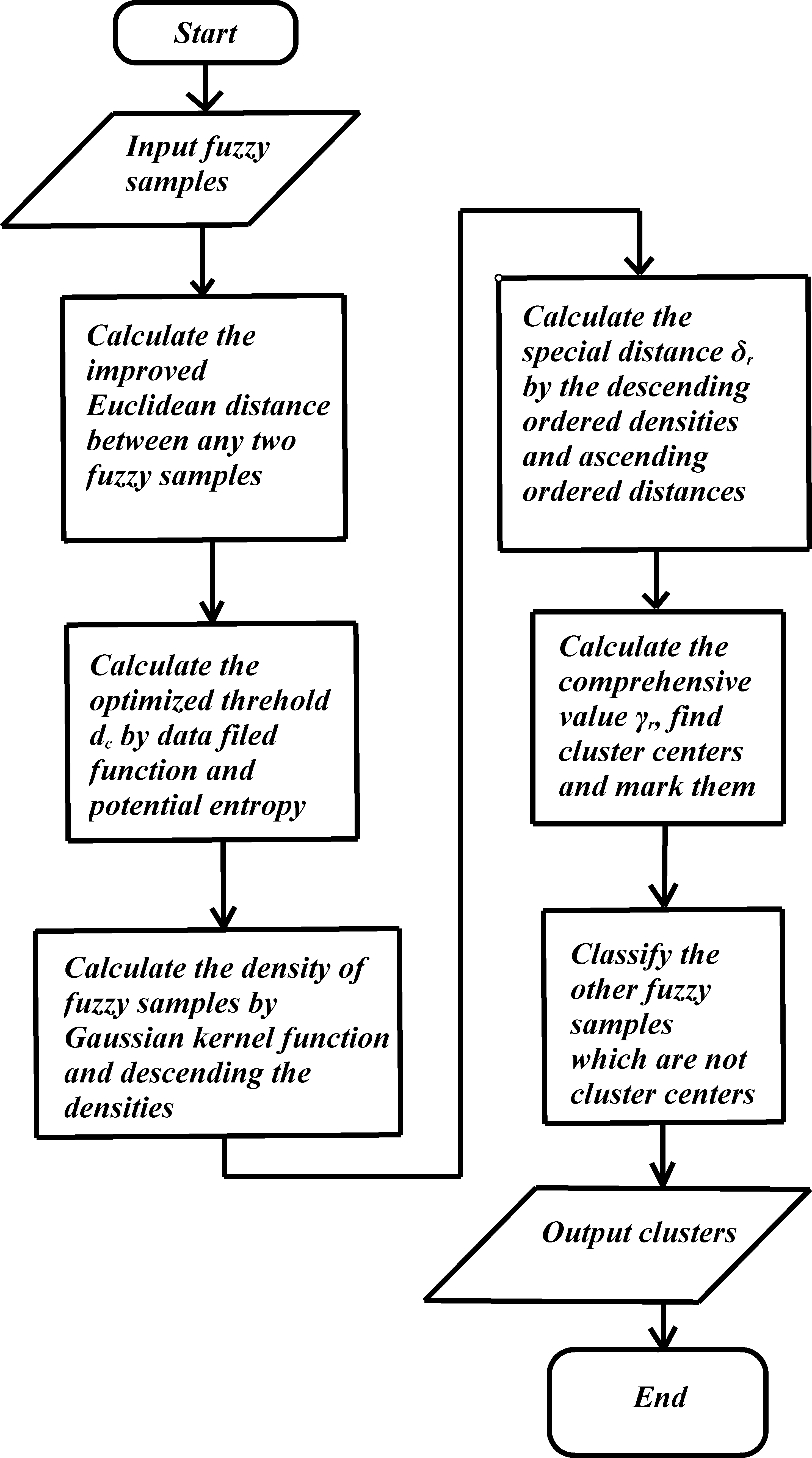
Calculate the improved Euclidean distance between any two fuzzy samples by Eqs (7), (10)–(12)
Calculate the optimized threshold by Eqs (13)–(15)
Calculate the density of fuzzy samples by Eq. (16), descending the densities
Calculate the special distance by descending the ordered densities and Eq. (17)
Calculate the comprehensive value by Eq. (18) and find cluster centers, mark them by Eq. (19)
Classify the other fuzzy samples which are not cluster centers
In addition to Table 2, the flowchart of the FMTD-CFSFDP algorithm is given in Fig. 1.
Flowchart of the FMTD-CFSFDP algorithm.
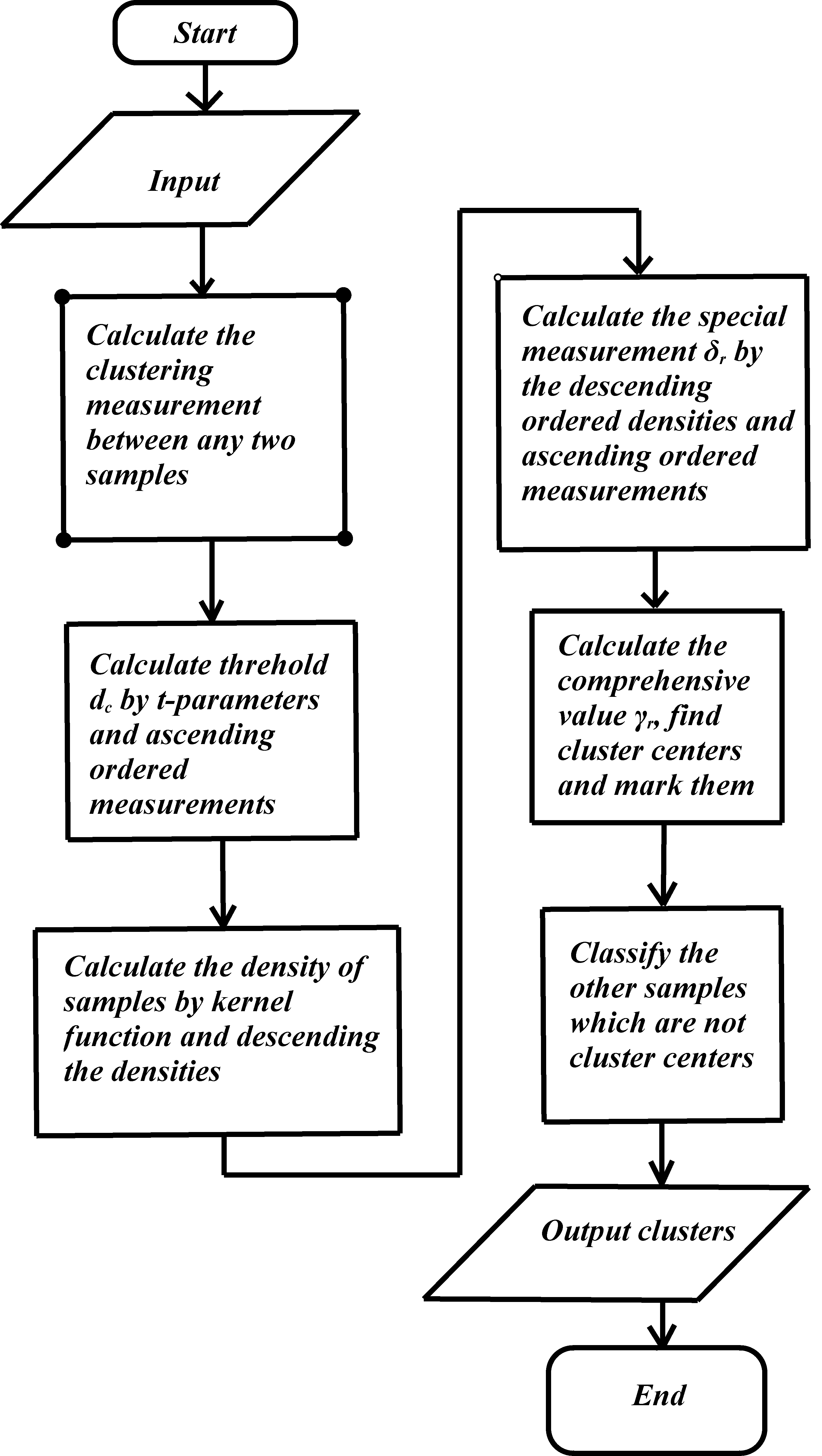
In order to compare with the FMTD-CFSFDP algorithm, the framework and flowchart of the original CFSFDP algorithm are listed here. The framework of CFSFDP is shown in Table 3.
Framework of CFSFDP
Algorithm: CFSFDP
Input: classical samples with classical data, the number of ples is , the number of indexes is , if the number of clusters are designated manually, then we input the designated number of cluster which is , otherwise, the input of is unn- ecessary. The -parameters are necessary to calculate the threshold,
Output: several clusters and clustering results
Calculate the measurement between any two samples by Minkowski distance or similarity degree
Calculate the threshold by ascending measurement and -parameters
Calculate the density of the sample by the cut-off kernel
function, Gaussian kernel function or exponential kernel function, descending the densities
Calculate the special measurement by descending ordered densities and ascending ordered measurement
Calculate the comprehensive value , find cluster centers and mark them
Classify the other classical samples which are not cluster centers
Obviously, from the framework and flowchart of the two algorithms, there is not much difference between FMTD-CFSFDP and CFSFDP in form. The difference between the algorithms is mainly reflected in the clustering objects, measurement calculating, parameters and threshold calculating. Furthermore, analyzing the time complexity for FMTD-CFSFDP, we listed the maximum time complexity of the clustering steps, parameters and key equations in Table 4.
Classify the other fuzzy samples which are not cluster centers
Output
Different clusters
Because the whole FMTD-CFSFDP algorithm is executed in a sequential manner, the maximum time complexity of FMTD-CFSFDP is . The time complexity of CFSFDP is [41]. In this case, it can be seen that the FMTD-CFSFDP algorithm has a higher time complexity than the CFSFDP algorithm. Next, we listed some algorithms in detail which relate to the CFSFDP algorithm or are improvements on the CFSFDP algorithm. Including CFSFDP and FMTD-CFSFDP, there are 11 kinds of clustering algorithm compared in Table 5.
Related algorithm comparing
Algorithm Name (Including Abbreviation)
Five key features/steps of the algorithm: 1) clustering objects; 2) measurement; 3) threshold; 4) density function; 5) method for identifying the number of clusters.
For classical data, the algorithm uses Euclidean distance as measurement, cut-off distance as the threshold, cut-off kernel as the density function, and identifies the number of clusters via decision graphs.
For classical data, the algorithm uses Euclidean distance as measurement, cut-off distance as the threshold, cut-off kernel as the density function, and identifies the number of clusters by expected cluster centers and standard deviation of special distance (equivalent to Eq. (17)).
For classical data, the algorithm uses Manifold distance as measurement, then, cut-off distance based on manifold distance and standard deviation to calculate the threshold, cut-off kernel as the density function, and identifies the number of clusters via fuzzy rules.
For classical data, the algorithm uses Euclidean distance as measurement, then, cut-off distance based on manifold distance and standard deviation to calculate the threshold, using cut-off kernel as the density function, and identifies the number of clusters by a “bump point” in decreasing ordered comprehensive value (equivalent to Eq. (18)).
Automatically selecting cluster centers in CFSFDP [28]
For classical data, the algorithm uses Euclidean distance as measurement, then, field function and potential entropy to calculate the threshold, a Gaussian kernel as the density function, and identifies the number of clusters by decision graphs and turning points.
For wireless sensor networks (WSN for short, the data for WSN are also classical data), the algorithm uses transmission distance as measurement, then, the algorithm uses the dynamic cut-off distance as the threshold, using density-energy defined in this article as the density function, and identifies the number of clusters by a new comprehensive value which is multiplied by the “residual energy of node”.
For THz spectra data (THz spectra data are also classical data), the measurement calculated by the dataset after dimension reduction processing with PCA, then, the algorithm uses cut-off distance as the threshold, a Gaussian kernel as the density function, and identifies the number of clusters by decision graphs.
For samples with multi-dimensional classical data, the algorithm uses weighted mixed Euclidean distance as measurement, then, field function and potential entropy to calculate the optimal threshold, a Gaussian kernel as the density function, and identifies the number of clusters by decision graphs.
For received signal strength indication (RSSI for short, the data for RSSI are also classical data), the algorithm uses Euclidean distance as measurement, then, the algorithm uses cut-off distance (which is different to CFSFDP in terms of the parameters’ value range) as the threshold, cut-off kernel as the density function, and identifies the number of clusters by decision graphs.
For interval data (a kind of uncertain classical data), the algorithm uses -ML distance proposed in this reference as measurement, then, the algorithm uses a grid density threshold, using the average density of the mesh, and identifies the number of clusters by decision graphs.
FMTD-CFSFDP (proposed in this article)
For fuzzy samples with fuzzy continuous sets and discrete fuzzy sets, the algorithm uses weighted mixed improved Euclidean distance (“improved Euclidean distance” for short) as measurement, then, field function and potential entropy to calculate the optimal threshold, a Gaussian kernel as the density function, and identifies the number of clusters by decision graphs.
Obviously, the main difference between FMTD-CFSFDP and the other algorithms is the type of clustering objects: the other algorithms focus on classical data, whereas FMTD-CFSFDP involves fuzzy mixed data.
Random simulations
Subsequently, four sets of random simulations in total were conducted, with the simulation conditions listed in Table 6.
Simulation conditions
Parameters
Values
Hardware
CPU
AMD Athlon (tm) II X4 630 Processor
CPU Clock Speed
2.80 GHz
Memory
4.00 GB
Software
OS
Windows 7 Home Basic
Tool
R version 2.15.1 (2012-06-22)
Tables 7–10 list the relevant information for the four sets of simulations, in which R denotes the fetching rule and T denotes the parameter type. “Fetching rule” represents the rules for generating clustering objects in random simulation. For a detailed explanation of these simulations, see Appendix 2.
Relevant information for the first set of simulation
200
Index ( 2, 1)
3
Index A
Index B
Index C
2
Normal fuzzy set
Normal fuzzy set
Discrete fuzzy set
Cluster 1
T
R
Cluster 2
T
R
Value range of the fuzzy set
Domain of discourse
Relevant information for the second set of simulation
300
Index ( 2, 1)
3
Index A
Index B
Index C
3
Normal fuzzy set
Normal fuzzy set
Discrete fuzzy set
Cluster 1
T
R
Cluster 2
T
R
Cluster 3
T
R
Value range of the fuzzy set
Discourse of the domain
Relevant information for the third set of simulation
300
Index ( 2, 1)
3
Index A
Index B
Index C
3
Normal fuzzy set
Normal fuzzy set
Discrete fuzzy set
Cluster 1
T
R
Cluster 2
T
R
Cluster 3
T
R
Value range of the fuzzy set
Discourse of the domain
Relevant information for the fourth set of simulation
300
Index ( 1, 2)
3
Index A
Index B
Index C
3
Normal fuzzy set
Discrete fuzzy set
Discrete fuzzy set
Cluster 1
T
R
Cluster 2
T
R
Cluster 3
T
R
Value range of the fuzzy set
Discourse of the domain
After four random simulations (25 runs per group), the decision graphs are plotted(choose one from random simulation of each group), as shown in Fig. 3(a)–(d). These describe the relations between the comprehensive measure value for automatically identifying the number of clusters and the corresponding serial number of the sample after the arrangement of in descending order. Specifically, the y-axis represents in descending order and the x-axis is the corresponding . According to the explanation in the CFSFDP algorithm, the value at the cluster center will form a jump point, but will be smoother at a non-clustered center will be smoother. Therefore, the cluster center can be found by searching for the jump point. The specific details and methods are described in [24].
Decision graphs of the simulation results after the arrangement of in descending order.
The present clustering results are verified and evaluated using the definition of clustering accuracy proposed by Al-Shammary et al. in [44]. According to this definition, the clustering accuracy of the algorithm on the sample set can be calculated as Eq. (20):
where denotes the number of real clusters in the sample set, denotes the number of correctly-classified samples in the -th cluster and denotes the number of samples. A greater value of suggests a more favorable clustering performance. Equation (20) represents the overall clustering accuracy. However, it is difficult to determine a range of clustering accuracies that correspond to a good clustering, as this depends on concrete conditions and clustering requirements. For example, if a task has a man-made threshold of 50.00% for the overall accuracy of the algorithm, naturally, clustering accuracy of more than 50.00% is considered to be a better performance less than 50.00% is considered as poor performance. In theory, without considering the complexity of the algorithm, the higher the clustering accuracy, the better.
Then, in accordance with the arrangement of and the clustering results, the threshold value and clustering accuracy are calculated, as shown in Tables 11–14. The mean of clustering accuracy rate is abbreviated as MC. Variance of the clustering accuracy rate is abbreviated as VC.
Summary of the clustering results for the first sets of simulations
Experiment
number
Optimal
threshold
Clustering
accuracy (%)
Experiment
number
Optimal
threshold
Clustering
accuracy (%)
1
0.89
52.00
14
0.97
50.50
2
0.91
51.00
15
0.89
51.00
3
0.94
52.00
16
0.93
55.00
4
0.93
51.00
17
0.94
52.50
5
0.83
54.00
18
0.91
55.50
6
0.81
50.50
19
0.85
52.50
7
0.90
50.00
20
0.87
51.50
8
0.94
52.50
21
0.87
54.50
9
0.92
52.00
22
0.85
55.00
10
0.89
51.00
23
0.91
56.50
11
0.84
52.00
24
0.89
50.00
12
0.89
50.00
25
0.88
56.00
13
0.84
50.50
MC 52.36% VC 4.0525
Summary of the clustering results for the second sets of simulations
Experiment
number
Optimal
threshold
Clustering
accuracy (%)
Experiment
number
Optimal
threshold
Clustering
accuracy (%)
1
0.38
40.67
14
0.40
37.00
2
0.39
41.67
15
0.41
35.67
3
0.40
36.33
16
0.39
37.33
4
0.39
36.33
17
0.41
33.67
5
0.40
38.67
18
0.40
37.33
6
0.39
39.00
19
0.38
36.00
7
0.41
37.00
20
0.40
39.67
8
0.39
46.33
21
0.40
38.33
9
0.40
38.00
22
0.39
39.00
10
0.38
40.33
23
0.40
42.67
11
0.39
38.00
24
0.40
34.67
12
0.38
42.00
25
0.39
37.67
13
0.39
41.00
MC 38.57% VC 7.7999
Summary of the clustering results for the third sets of simulations
Experiment
number
Optimal
threshold
Clustering
accuracy (%)
Experiment
number
Optimal
threshold
Clustering
accuracy (%)
1
0.88
46.33
14
0.79
53.67
2
0.87
40.67
15
0.82
54.33
3
0.76
41.33
16
0.80
48.00
4
0.77
39.33
17
0.74
52.67
5
0.79
45.00
18
0.71
53.67
6
0.56
47.67
19
0.91
45.00
7
0.76
38.00
20
0.83
40.67
8
0.72
39.33
21
0.70
43.33
9
0.77
46.33
22
0.84
41.33
10
0.47
40.00
23
0.87
50.67
11
0.50
45.00
24
0.86
56.33
12
0.78
38.67
25
0.76
45.00
13
0.80
43.67
MC 45.44 VC 29.96
Summary of the clustering results for the fourth sets of simulations
Experiment
number
Optimal
threshold
Clustering
accuracy (%)
Experiment
number
Optimal
threshold
Clustering
accuracy (%)
1
3.08
37.67
14
3.06
35.33
2
3.09
36.67
15
3.11
37.00
3
3.04
36.67
16
3.07
37.33
4
3.02
35.00
17
3.13
38.00
5
2.98
35.00
18
3.05
36.33
6
3.09
36.67
19
3.02
38.33
7
3.08
38.33
20
3.08
39.00
8
3.10
38.33
21
3.08
36.67
9
3.16
35.00
22
3.07
36.67
10
3.10
39.33
23
3.02
35.00
11
3.07
37.67
24
3.06
37.00
12
3.06
37.67
25
3.08
35.00
13
3.04
37.33
MC 36.92 VC 1.71
Through 100 artificial random fuzzy sample sets, it can be seen from the clustering results that the clustering accuracy span is very large, ranging from more than 30.00% to less than 60.00%. This may be due to the differences between the sample sets themselves, or the clustering accuracy of the algorithm is not stable enough. Obviously, the clustering accuracy of the first set of simulations and the third set of simulations is higher than that of the second and fourth sets.
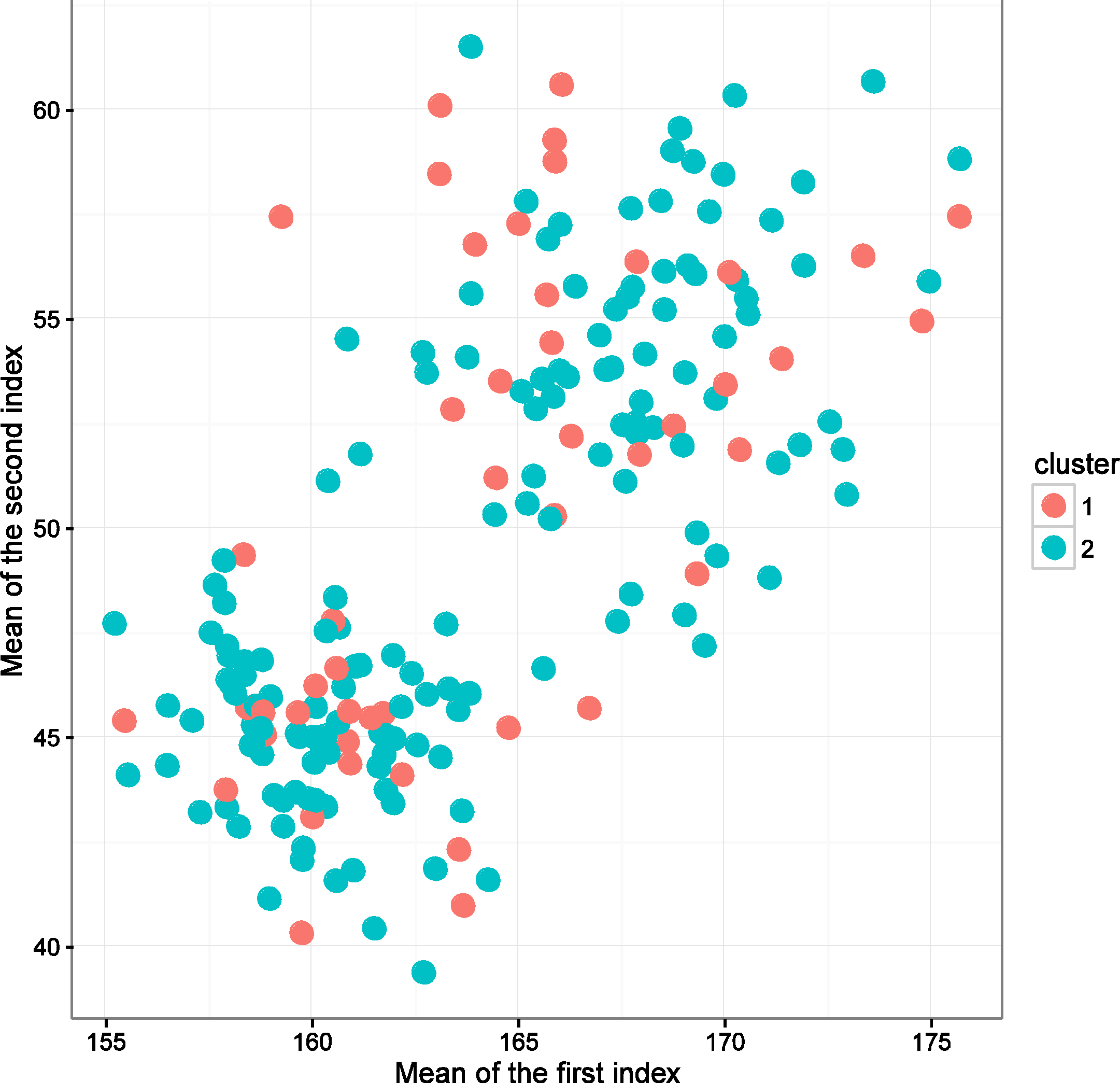
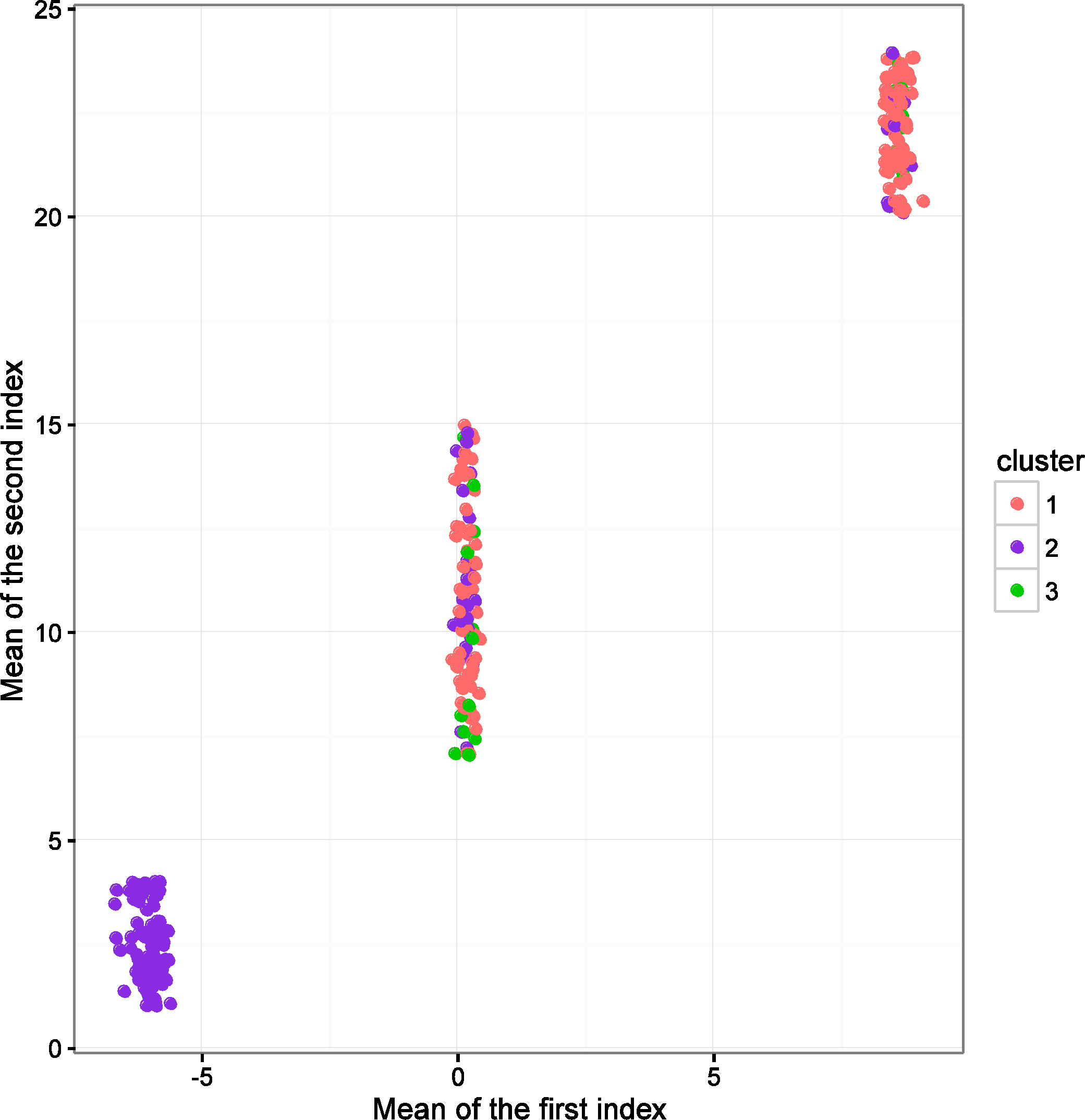
Taking advantage of the experimental conditions of the first and third sets of simulations, two fuzzy sample sets with mixed data are generated randomly by experimental conditions which have been mentioned above, and then recorded as FMTDS-1 and FMTDS-2. For these, the clustering accuracy of FMTDS-1 is 52.50% and the accuracy of FMTDS-2 is 63.67%. To further demonstrate the clustering effect, we attempt to draw the clustering results of these two sets of fuzzy sample sets. For a fuzzy sample composed of several continuous fuzzy sets and discrete fuzzy sets, it is difficult to draw the clustering result directly. This is because, in the simulations, the first index and the second index correspond to continuous fuzzy sets, and normal fuzzy sets are used. In this case, we can use the mean of the normal fuzzy set under the first index as the horizontal axis, and the mean of the normal fuzzy set under the second index as the vertical axis to draw the clustering result. As for the discrete fuzzy sets corresponding to the third index, this usually represents attributes, and for all the fuzzy samples in the simulation, elements in discrete fuzzy sets are identical, but the degree of membership of elements to discrete fuzzy sets is different. In short, the types and numbers of attributes possessed by the fuzzy samples are the same, but to different degrees of membership.
When graphing, the attributes of different membership degrees can be represented by different colors, provided that there are enough kinds of tones and that they are easily distinguished by human vision. However, it is difficult to satisfy this requirement because sometimes human vision cannot distinguish the subtle differences between two similar colors. As there are hundreds of samples in each simulation, which require hundreds of colors, this inevitably makes the differentiation between some colors. Moreover, because we need to use color to represent samples in different clusters in two-dimensional graph, to avoid confusion, it is impossible to use color to represent discrete fuzzy sets again. Therefore, discrete fuzzy sets can be omitted for the time being in this example. Because there is no difference between elements in discrete fuzzy sets, the difference only exists in the membership degree of elements to discrete sets; therefore, if we mark elements in discrete fuzzy sets on the axes, all samples are the same, which can not reflect any differences. Even if we consider drawing the membership of elements in discrete fuzzy sets on a numbered axis, because the membership degree is between 0 and 1, the difference between different fuzzy samples reflected on the two-dimensional map is still insignificant. Because there is no such problem in normal fuzzy sets, the elements themselves are infinite, and the mean value is the key parameter which can represent them to some extent; therefore, in a fuzzy samples with two continuous fuzzy sets and one discrete fuzzy set, we only consider drawing the mean values of two continuous fuzzy sets on the horizontal and vertical axes, and replacing this fuzzy samples with a coordinate point composed of two mean values. According to the above rules, the clustering results of FMTDS-1 and FMTDS-2 are shown in Figs 4 and 5, respectively.
Clustering result for FMTDS-1.
Clustering result for FMTDS-2.
Obviously, as the clustering accuracy reflects, the clustering effect of FMTDS-2 is better than that of FMTDS-1.
Conclusions
As shown in Fig. 3 and Tables 11–14, the CFSFDP algorithm that automatically identifies the number of clusters by searching for the jump points of , only performs successfully in the first set of simulations and fails in the other sets of simulations. As a result, the accuracy for certain simulations is not high. This suggests that, when using FMTD-CFSFDP algorithm, the automatic identification of the number of clusters based on the jump point of is unstable and easily fails. Since the improved Euclidean distances between continuous fuzzy sets or discrete fuzzy sets are calculated based on membership degrees with a range of [0, 1], the calculated improved Euclidean distances are always small. The overall distance as well as the threshold value are small, thereby resulting in small calculated values of and (corresponding to the density of fuzzy samples and special distance). Accordingly, the acquired comprehensive measure value is also small. Although it is not the only reason, the value range of the membership degrees within [0, 1] can easily result in a discrimination degree that is too low, i.e., it is difficult to determine the number of clusters based only on the visual identification of the jump point of . By referring to [24], the clustering accuracy obtained by the FMTD-CFSFDP algorithm is lower than that using CFSFDP algorithm, which can be attributed to the introduction of the concept of fuzzy sets. Accordingly, each state (i.e., each element) corresponding to each index of the sample in the fuzzy set can be treated as a number. In other words, although each sample theoretically includes two or three fuzzy sets in the four sets of random simulations, nearly all elements in each fuzzy set are used in calculating the related parameters, i.e., a large number of elements (without limits) in any a continuous fuzzy set are involved in the calculation. Therefore, the FMTD-CFSFDP algorithm contains much more information than CFSFDP on classical sets, thereby yielding lower clustering accuracy.
In summary, FMTD-CFSFDP algorithm is applicable to the clustering of samples with fuzzy mixed data, which also inherits most of the advantages of the CFSFDP algorithm. The main innovation of this study lies in the extension of the CFSFDP algorithm from classical sets to fuzzy sets. Accordingly, a novel clustering algorithm for fuzzy mixed data is proposed, the mathematical definition of fuzzy mixed data is provided, and the Euclidean distance between fuzzy samples is improved so as to reduce errors.
Discussion
However, in spite of the above innovations mentioned in Section 5, the proposed FMTD-CFSFDP algorithm still exhibits the following three limitations. Firstly, using the FMTD-CFSFDP algorithm, fuzzy samples cover the information of the fuzzy sets, but the membership of fuzzy samples to the cluster still follows hard division without the consideration of fuzzy characteristics. Many of the calculations involve fuzzy mathematics, including the calculation of fuzzy nearness, fuzzy degrees and fuzzy distance, which are converted into classical quantities and finally classical values are output. Although the above calculations are reasonable in fuzzy mathematics, some information is always lost during the conversion from fuzzy sets to classical sets. In particular, a hard division of fuzzy samples can reduce the clustering accuracy to certain degree. Secondly, in this study, the improved Euclidean distance is proposed, which exhibits less error than the traditional Euclidean distance, and the overall distance is calculated after weighting. However, the distances cannot be calculated without the membership degree. The membership degree ranges from 0 to 1, which will undoubtedly weaken the discrimination degree of the overall distance, thereby resulting in a decrease of clustering accuracy compared to the results for CFSFDP. Thirdly, the proposed FMTD-CFSFDP algorithm fails to overcome the shortcoming of the CFSFDP algorithm in the visual identification of cluster numbers and makes the identification of the number of clusters more unstable (see Fig. 3, this point has been mentioned in the previous simulation experiments of Section 4). This can be partly attributed to the decrease in the discrimination degree of the measure as described above. Because of this low discrimination degree, the value of for the final automatic identification of the number of clusters varies slightly and thus cannot be effectively discriminated using visual means.
Based on the above analysis, the FMTD-CFSFDP algorithm can be further improved based on the following aspects. Firstly, the membership between fuzzy samples and clusters should also be defined on fuzzy sets so that both the sample information and memberships are established on fuzzy sets. By doing so, information loss in clustering and classification may be reduced so as to enhance clustering accuracy. Secondly, the fuzzy distance calculated based on membership degrees and all related improvements should be abandoned and a new measure that reflects fuzzy data characteristics should be developed. Thirdly, a novel identification method for the number of cluster should be sought for replacing the visual identification based on the characteristics of in the geometrical images, i.e., a set of quantized mathematical models should be proposed for the automatic identification of the number of clusters. Accordingly, the second and third shortcomings described above can be overcome and even subtle differences can be easily identified by the established mathematical model, so as to enhance the discrimination degree in clustering. Overall, the present research can provide insightful direction for further clustering on fuzzy sets.
Footnotes
Appendix 1
With regard to Eq. (6), assuming that , and represent the overall error, systematic error and random error, respectively, the following expression can be derived:
For Eq. (7), assuming that , and represent the overall error, systematic error and random error, respectively, the following expression can be derived:
It should be noted that all the errors are nonnegative. For comparing and , since the random error cannot be artificially controlled and it can be assumed that , only and should be compared. Assuming that denotes the error of , since , for the -th index, denotes the public integration domain. Obviously, according to the property of definite integration, for the fuzzy set or of each fuzzy sample, in a non-integration domain: 0, or 0, and . In other words, for and , the integration in a non-public integration domain can be calculated as , and ( represents the difference set, i.e., the integration domain of except . For a single index, the error only exists in the defined integration domain, while the integrations in a non-defined non-integration domain are all equal to 0, suggesting no error. Accordingly, the following expression can be derived:
The systematic error of Eq. (6) can then be calculated as:
Based on the property of definite integration,
and the systematical error of Eq. (7) can be calculated as:
Apparently, . Since , . The error of the improved Euclidean distance according to Eq. (7) is smaller than that calculated according to Eq. (6).
Appendix 2
In the first set of simulations, 200 fuzzy samples were used, and each sample includes three indexes (i.e., 200 and 3). Specifically, two indexes (Index A and Index B) are continuous fuzzy subsets in the discourse domain and one index is a discrete fuzzy subset (Index C) in (i.e., 2 and 1). These samples were artificially divided into two clusters in advance, i.e., 2. For the first 100 samples in a cluster, assuming that the two continuous fuzzy subsets are normal fuzzy sets, the parameters and in the membership function corresponding to Index A are from the two normal distributions and , and the parameters and in the membership function corresponding to Index B are also from the two normal distributions and . With regard to Index C (a discrete fuzzy set), a set was first obtained by arbitrarily setting and ; assuming , the membership degree of to the discrete fuzzy set (Index can be determined by the uniform distribution . It should be noted that the distributions can be arbitrary, which only represent a fetching rule. The remaining 100 samples are in another cluster; the parameters and in the membership function corresponding to Index A are described by the two normal distributions and , the parameters and in the membership function corresponding to Index B are described by the two normal distributions and , and the membership degrees of the five elements corresponding to Index C ( to the discrete fuzzy set C can be generated by the uniform distribution .
The second set of simulations includes 300 normal fuzzy samples in total ( 300), in which each sample has three indexes ( 3). Similar to the condition in the first set of simulation, the three indexes include two continuous fuzzy subsets in the domain of discourse , denoted as Index A and Index B, and one discrete fuzzy subset, denoted as Index C. Accordingly, 2 and 1. These 300 fuzzy samples were artificially divided into three clusters in advance (i.e., 3). For the first 100 samples in a cluster, this study also assumes that the two continuous fuzzy subsets are normal fuzzy sets; specifically, the parameters and in the membership function corresponding to Index A are described by the two normal distributions and , and the parameters and in the membership function corresponding to Index B are described by the two normal distributions and . For Index C (a discrete fuzzy set), a set was first obtained by arbitrarily setting and , and then, assuming , the membership degree of to the discrete fuzzy set (Index ) can be described by the uniform distribution (. The middle samples are in a cluster; the parameters and in the membership function corresponding to Index A are from the two normal distributions and , the parameters and in the membership function corresponding to Index B are from the two normal distributions and , and the membership degrees of the three elements corresponding to Index C ( to the discrete fuzzy set are generated by the uniform distribution . The remaining 100 samples are in a cluster; the parameters and in the membership function corresponding to Index A are from the two normal distributions and , the parameters and in the membership function corresponding to Index B are described by the two normal distributions and , and the membership degrees of the three elements corresponding to Index C ( to the discrete fuzzy set are generated by the uniform distribution .
In the third set of simulations, 300 fuzzy samples and three indexes in total are involved (i.e., 300 and 3). Specifically, these three indexes are two continuous fuzzy subsets in the domain of discourse , dented as Index A and Index B, and one discrete subset in the domain of discourse denoted as Index C, i.e., 2 and 1. Similarly, these fuzzy samples are artificially classified into three clusters, i.e., . The first 100 samples are in a cluster. Firstly, this study also assumes that the two continuous fuzzy subsets are normal fuzzy sets: the parameters and in the membership function corresponding to Index A are from a normal distribution and an exponential distribution while the parameters and in the membership function corresponding to Index B are described by the two uniform distributions and ; for Index C (a discrete fuzzy set), a set can first be obtained by arbitrarily setting and , and then, assuming , the membership degree of to the discrete fuzzy set (Index can be generated by the uniform distribution . The middle samples are in a cluster; the parameters and in the membership function corresponding to Index A are from a normal distribution and an exponential distribution , the parameters and in the membership function corresponding to Index B are from two uniform distributions and , and the membership degrees of the four elements corresponding to Index C ( to the discrete fuzzy set are generated by the uniform distribution . The remaining 100 samples are in a cluster; the parameters and in the membership function corresponding to Index A are from a normal distribution and an exponential distribution , the parameters and in the membership function corresponding to Index B are described by the two uniform distributions and , and the membership degrees of the four elements corresponding to Index C to the discrete fuzzy set ( are generated by the uniform distribution .
The fourth set of simulations includes 300 fuzzy samples and three indexes (i.e., 300 and 3). Similarly, for the three indexes, one index is for the continuous fuzzy subsets in the domain of discourse , denoted as Index A, and the other two indexes are discrete fuzzy subsets in , denoted as Index B and Index C, i.e., 1 and 2. The 300 samples are artificially divided into three clusters ( 3). As to the first 100 sample in a cluster, this study also assumes that the continuous fuzzy subset is a normal fuzzy set; specifically, the parameters and in the membership function corresponding to Index A are from the two normal distributions and ; for Index B (a discrete fuzzy set), a set can first be obtained by arbitrarily setting and , and then, assuming , the membership degree of to the discrete fuzzy set (Index ) can be generated by the uniform distribution ; for Index (a discrete fuzzy set), a set can first be obtained by arbitrarily setting and , and then assuming , the membership degree of to the discrete fuzzy set (Index ) can be generated by the uniform distribution (. The middle samples are in a cluster; the parameters and in the membership function corresponding to Index A are from the two normal distribution functions and , the membership degrees of four elements corresponding to Index B ( to the discrete fuzzy set are generated by the uniform distribution , and the membership degrees of the three elements corresponding to Index C ( to the discrete fuzzy set are also generated by the uniform distribution . The remaining 100 samples are in a cluster; the parameters and in the membership function corresponding to Index A are from the two normal distributions and , the membership degrees of four elements corresponding to Index B ( to the discrete fuzzy set are generated by the uniform distribution , and the membership degrees of the three elements corresponding to Index C ( to the discrete fuzzy set are generated by the uniform distribution .
References
1.
HanJ.W.KamberM. and PeiJ., Cluster analysis: Basic concepts and methods, in: Data Mining: Concept and TechniqueFanM. and MengX.F., transl., China Machine Press, Beijing, 2012, pp. 288–291.
2.
BishopC.M., Clustering algorithms, in: Neural Networks for Pattern Recognition, Clarendon Press, Oxford, 1995, pp. 187–189.
3.
ChenC.T., Research on K-modes Clustering Algorithm of Dissimilarity Measure, MSc. Dissertation, Taiyuan University of Technology, 2012.
4.
MacqueenJ., On convergence of K-means and partitions with minimum average variance, Annals of Mathematical Statistics36(3) (1965), 1084–1084.
5.
ChaturvediA.GreenP.E. and CarrollJ.D., K-modes clustering, Journal of Classification18(1) (2001), 35–55.
6.
KarbachW. et al., Model-K-prototyping at the knowledge level, Expert Systems with Application4(2) (1992), 268–268.
7.
ReynoldsA.P.RichardsG. and Rayward-SmithV.J., The application of K-medoids and PAM to the clustering rules, in: Proceedings of 2004 Intelligent Data Engineering and Automated Learning Ideal, 2004, pp. 173–178.
8.
MaR.N.WangX.L. and DingJ.D., Multilevel core-sets based aggregation clustering algorithm, Journal of Software24(3) (2013), 490–506.
9.
GuhaS.RastogiR. and ShimK., Rock: A robust clustering algorithm for categorical attributes, Information Systems25(5) (2000), 345–366.
10.
WilcoxH. et al., Simulation tests of galaxy cluster constraints on chameleon gravity, Monthly Notices of the Royal Astronomical Society462(1) (2016), 715–725.
11.
LorbeerB. et al., Variations on the clustering algorithm BIRCH, Big Data Research11 (2018), 44–53.
12.
BenmouizaK. and CheknaneA., Density-based spatial clustering of application with noise algorithm for the classification of solar, in: Proceedings of 2016 8th International Conference on Modelling, Identification & Control, 2016, pp. 279–283.
13.
BryantA. and CiosK., RNN-DBSCAN: a density-based clustering algorithm using reverse nearest neighbor density estimates, IEEE Transactions on Knowledge and Data Engineering30(6) (2018), 1109–1121.
14.
KanagalaH.K. and KrishnaiahV.V.J.R., A comparative study of K-means, DBSCAN and OPTICS, in: Proceedings of 2016 International Conference on Computer Communication and Informatics, 2016.
15.
DatN.D. et al., Sting algorithm used English sentiment classification in a parallel environment, International Journal of Pattern Recognition and Artificial Intelligence31(7) (2017), 1–30.
16.
SheikholeslamiG.ChatterjeeS. and ZhangA.D., WaveCluster: a wavelet-based clustering approach for spatial data in very large databases, VLDB Journal8(3-4) (2000), 289–304.
17.
LiM.HolmesG. and PfahringerB., Clustering large datasets using Cobweb and K-means in tandem, in: Proceedings of 17th Annual Australian Conference on Artificial Intelligence, 2004, pp. 368–379.
ZhangX.P. et al., Spatial clustering with obstacles constraints by ant colony optimization and quantum particle swarm optimization, in: Proceedings of 2009 International Conference on Artificial Intelligence and Computational Intelligence, 2009.
20.
ZhangX.P. et al., Spatial clustering with obstacles constraints using PSO-DV and K-Medoids, in: Proceedings of 2008 3rd International Conference on Intelligent System and Knowledge Engineering, 2008.
21.
RoyP. and MandalJ.K., A delaunay triangulation preprocessing based fuzzy-encroachment graph clustering for large scale GIS, in: Proceedings of 2012 International Symposium on Electronic System Design, 2012, pp. 300–305.
22.
BuZ. et al., CAMAS: A cluster-aware multiagent system for attributed graph clustering, Information Fusion37 (2017), 10–21.
23.
ZakiM.J. et al., CLICKS: An effective algorithm for mining subspace clusters in categorical datasets, Data & Knowledge Engineering60(1) (2007), 51–70.
24.
RodriguezA. and LaioA., Clustering by fast search and find of density peaks, Science344(6191) (2014), 1492–1496.
25.
MehmoodR. et al., Fuzzy clustering by fast search and find of density peaks, in: Proceedings of 2015 International Conference on Identification, Information, and Knowledge in the Internet of Things, 2015.
26.
WanM. et al., Optimized fuzzy clustering by fast search and find of density peaks, in: Proceedings of 2018 IEEE 3rd International Conference on Cloud Computing and Big Data Analysis, 2018.
27.
GaoJ. et al., ICFS: An improved fast search and find of density peaks clustering algorithm, Proceedings of 14th IEEE Intl Conf on Dependable, Autonomic and Secure Comp/4th IEEE Intl Conf on Pervasive Intelligence and Comp/2nd IEEE Intl Conf on Big Data Intelligence and Comp/IEEE Cyber Sci and Technol Congress, 2016.
28.
ShenY.C. and ZhangH., Automatically selecting cluster centers in clustering by fast search and find of density peaks with data field, in: Proceedings of 2017 2nd International Conference on Information Systems Engineering, 2017.
29.
ZhangY.M.LiuM.D. and LiuQ.W., An energy-balanced clustering protocol based on an improved CFSFDP algorithm for wireless sensor networks, Sensors18(3) (2018).
30.
QinB.Y. et al., Terahertz time-domain spectroscopy combined with PCA-CFSFDP applied for pesticide detection, Optical and Quantum Electronics49(7) (2017).
31.
LiY.ChenY.Y. and ZhangS.F., Design of mixed data clustering algorithm based on density peak, Journal of Computer Application38(2) (2018), 483–490.
32.
LiY. and ChenY.Y., Evaluation on the annual development status of private hospitals in Mainland China based on Mao-CFSFDP clustering algorithm, Basic & Clinical Pharmacology & Toxicology123(3) (2018), 109–110.
33.
ZadehL.A., Fuzzy sets, Information and Control8(3) (1965), 338–353.
34.
BarniM.CappelliniV. and MecocciA., A possibilistic approach to clustering-comments, IEEE Transactions on fuzzy systems4(3) (1996), 393–396.
PalN.R. et al., A possibilistic fuzzy c-means clustering algorithm, Journal of Cybernetics3(3) (1974), 32–57.
37.
WangS. and ChenY., HASTA: A hierarchical-grid clustering algorithm with data field, International Journal of Data Warehousing and Mining10(2) (2014), 39–54.
38.
GeorgeJ.K. and BoY.A., Fuzzy sets: Basic concepts, in: Fuzzy Sets and Fuzzy Logic: Theory and ApplicationPattiG., ed., Prentice Hall PTR, New Jersey, 1995, pp. 19–30.
39.
ChenS.L.LiJ.G. and WangX.G., in: Fuzzy sets and membership function, in: The Theory of Fuzzy Sets and Its Application, Science Press, Beijing, 2005, pp. 28–42.
40.
HuangZ., Clustering large data sets with mixed numeric and categorical values, in: Proceedings of the First Pacific-Asia Knowledge Discovery and Data Mining Conference, 1997, pp. 39–54.
41.
ZhangW.K., Research on density-based hierarchical clustering algorithm, MSc. Dissertation, University of Science and Technology of China, 2015.
42.
LiuY.JiaD. and WangH.Z., Adaptive indoor localization algorithm of based on CFSFDP in complex environment, Journal of Signal Processing34(4) (2018), 465–475.
43.
HuJ.QinH. and MaoY.M., Application of uncertain GM-CFSFDP clustering algorithm in landslide hazard prediction, Computer Systems & Application27(6) (2018), 195–201.
44.
Al-ShammaryD. et al., Fractal self-similarity measurements based clustering technique for SOAP web messages, Journal of Parallel and Distributed Computing73(5) (2013), 664–676.