Label noise detection under the noise at random model with ensemble filters

Abstract

Label noise detection has been widely studied in Machine Learning because of its importance in improving training data quality. Satisfactory noise detection has been achieved by adopting ensembles of classifiers. In this approach, an instance is assigned as mislabeled if a high proportion of members in the pool misclassifies it. Previous authors have empirically evaluated this approach; nevertheless, they mostly assumed that label noise is generated completely at random in a dataset. This is a strong assumption since other types of label noise are feasible in practice and can influence noise detection results. This work investigates the performance of ensemble noise detection under two different noise models: the Noisy at Random (NAR), in which the probability of label noise depends on the instance class, in comparison to the Noisy Completely at Random model, in which the probability of label noise is entirely independent. In this setting, we investigate the effect of class distribution on noise detection performance since it changes the total noise level observed in a dataset under the NAR assumption. Further, an evaluation of the ensemble vote threshold is conducted to contrast with the most common approaches in the literature. In many performed experiments, choosing a noise generation model over another can lead to different results when considering aspects such as class imbalance and noise level ratio among different classes.

Keywords

Label noise noise detection ensemble methods noise at random ensemble noise filtering

1. Introduction

Data quality is of great importance for ML applications and, in particular, for classification tasks. Conventionally in these tasks, a training set of labeled instances is given as input to an ML algorithm, which will acquire useful knowledge to make predictions for new instances. In practice, real-world datasets frequently contain irregularities such as incompleteness, noise, and data inconsistencies that impact ML performance [15]. In this light, noise detection and filtering are quite relevant techniques for ML [31].

According to the literature, noise may occur in both attributes and classes [31]. This work focuses on the latter problem, in which an unknown proportion of instances in a dataset are mislabeled because of different reasons. This is a relevant problem since label noise can harm the identification of true class boundaries in a problem, increase the chance of overfitting, and affect learning performance in general [9].

Previous works successfully adopted the classification noise filtering method [7, 24, 14] for label noise detection, widespread in the literature. In this approach, mislabeled instances in a dataset are identified according to the output results of a classifier or an ensemble of classifiers. For example, in the majority vote for ensemble noise detection, an instance is marked as mislabeled if most classifiers in a pool incorrectly classify it. In the consensus vote for ensemble noise detection, a record is considered noisy if all classifiers in the pool misclassify it.

As with most ML tasks, empirical evaluation is also crucial in the context of noise detection techniques. Producing a ground-truth dataset for evaluation usually requires additional domain experts to decide which instances were mislabeled. This process can be costly, and experts are not always available. This problem is mitigated when artificial datasets are used or when simulated noise is injected into a dataset in a controlled way. The investigation of how noise influences the learning process is simplified when a systematic addition of noise is performed [11].

Label noise can be injected into a dataset by assuming three distinct models of noise [9]: (i) Noisy Completely at Random (NCAR), in which the probability of an instance being noisy is random, (ii) Noisy at Random (NAR), the probability of an instance being noisy depends on its label, and (iii) Non-Noisy at Random (NNAR), the probability of an instance being noisy also depends on its attributes. In many previous works [24, 7, 22, 11], a single noise model is chosen over another to perform experiments. Nevertheless, it is usually not clear how this choice can affect experimental results. Additionally, other aspects, like class distribution, can impact the distribution of noise differently in a dataset depending on the noise type considered. For instance, a human supervisor may find it more difficult to label records from the minority class than the majority class in some contexts.

In this work, it is investigated how noise models can influence noise detection experiments under different aspects. In contrast to previous studies, the influence of distinct label noise models on ensemble noise detection is evaluated in this research under various contexts such as class imbalance, noise distribution, ensemble thresholds, and percentage of noise in data. It is shown that different results are achieved depending on the context. For instance, even under the same noise model (e.g., NAR), a detection technique may have quite distinct performance results if class imbalance changes (e.g., NAR with imbalanced vs. NAR with balanced class distributions).

The remainder of this paper is organized as follows. In Section 2, an overview of label noise detection is presented. The proposed methodology is described in Section 3. Experiments are presented in Section 4. Finally, Section 5 summarizes the paper and presents future work.

2. Related works

In [31], two types of noise are distinguished for supervised learning datasets: attribute (or feature) and class (or label) noise. The former is present in one or more features due to absent, incorrect, or missing values. In turn, label noise can be generated because of many reasons, such as the low reliability of human experts during labeling, incomplete information, communication problems, among others [3]. The presence of noise in the training dataset can lead to an increase in processing time, higher model complexity, and the chance of overfitting, which will then deteriorate the predictive performance [19].

According to the literature, removing examples with feature noise is not as beneficial as label noise detection. This occurs since the values of non-noisy features can be helpful in the classification process and because there is only one label, while there are many attributes [9]. Besides, feature noise can later give rise to label noise. Hence, this work will concentrate on the label noise problems. From now on, label noise is also referred to as noise.

This section initially presents a brief review of standard label noise detection techniques in the literature (Section 2.1). Previous works have commonly evaluated such methods by performing experiments in which noise is intentionally injected into a dataset. A model is required in these experiments to control how the label noise is distributed across the dataset instances. Different label noise models are presented in Section 2.2. Finally, the scope of this paper and its contributions are presented in Section 2.3.

2.1 Noise detection approaches

Several techniques have already been developed for dealing with label noise. According to [9], two broad strategies can be used: (1) the algorithm-level strategy, i.e., designing classifiers that are more robust and noise-tolerant, and (2) the data-level strategy, i.e., performing data cleaning by filtering noisy instances as a preprocessing step.

2.1.1 Algorithm-level approach

Some learning algorithms are naturally more tolerant to noise, which can be used as a benefit in the presence of label noise. Ensemble methods like bagging have the diversity increased when noise is present, which helps to cope with mislabeled examples. The decision tree pruning process is also more robust to noisy data as it has been shown that this technique decreases the influence of label noise since it prevents data overfitting [1].

Even more robust learning algorithms can be derived by including the noise information during the learning process. In [5], for example, it is proposed the generalized robust Logistic Regression (gLR), in which the exponential distribution was adopted to model noise in such a way that points closer to the decision boundary have a relatively higher chance of being mislabeled. In the robust Kernel Fisher Discriminant[18], a probability of the label being noisy is derived by applying an Expectation-Maximization algorithm. In the robust kernel logistic regression[6], the optimal hyperparameters of the method are automatically determined using Multiple Kernel Learning and Bayesian regularization techniques. In [5], a logistic regression classifier is built by employing a noise model based on a mixture of Gaussians. In [4], the Label Noise robust SVMs deal with noise present in data by correcting the kernel matrix with a specially structured matrix based on the information regarding the level of noise in the dataset.

The approaches above directly model label noise during the learning process. Although the advantage of those methods is to use prior knowledge regarding a noise model and its consequences [9], it increases the complexity of learning algorithms and can lead to overfitting, because of the additional parameters of the training data model.

2.1.2 Data-level approach

While the algorithm-level strategy aims to implement robust models using some available information related to the noise present in data, the data-level approach handles noisy data before the training process. The algorithm-level methods are less versatile, as not all algorithms have robust versions. In turn, the data-level strategy has the advantage of considering the noise filtering and the learning phase as distinct steps. Hence, it avoids using polluted instances during the learning process, improving both predictive performance and computational cost. Also, filtering approaches are usually cheap and easy to implement [9]. Thus, our work will be focused on the data-level category.

Label noise filtering can be performed in a variety of ways. For example: by using complexity measures for the records [26, 25]; partitioning approaches for removing mislabeled instances in large datasets [32, 12]; filtering noisy examples by verifying the impact of the removal on the learning process [20]; using neighborhood-based algorithms to remove instances that are distant from the ones of the same class [29, 16], among others.

In our work, we adopted the ensemble approach for noise filtering, in which instances are removed when a certain number of algorithms misclassifies them [30]. This approach has been widely chosen [7, 32, 28, 3, 23, 22, 30, 14], as it overcomes the problem of relying on a single classifier for noise filtering. Using only one classifier for noise filtering can cause the removal of too many instances. The ensemble approach improves noise detection since an instance is likely to have been incorrectly labeled if distinct classifiers disagree on their predictions. The ensemble noise filtering applies the $k$ -fold cross-validation, i.e., in $k$ repetitions, $k-1$ folds of the dataset are used for training each algorithm in the ensemble, and the remaining fold is used for validation. Then, all records are classified by all algorithms in the pool, and the observed errors are taking into account to remove instances.

An essential issue in ensemble-based noise filtering is how many misclassifications are assumed to consider an instance as noisy. There are two common choices in the literature: the consensus and the majority vote [14, 24, 30]. Whereas the majority vote classifies an instance as incorrectly labeled if a majority of the algorithms in the pool misclassifies it, the consensus vote requires that all classifiers have misclassified the record. These vote techniques can produce different results. As the consensus requires a higher agreement of classifiers, it tends to remove a few instances. On the other hand, the majority vote may throw out too many instances, including noise-free ones that could be relevant.

The trade-off between choosing the majority or the consensus approach can be replaced by the problem of selecting a vote threshold. The majority and the consensus vote are special cases, when thresholds are 50% and 100%, respectively. The adequate vote threshold would be related to the expected proportion of noisy instances in a dataset. Nevertheless, few works have investigated the influence of varying the vote thresholds. For example, in [17, 21], the authors showed that selecting appropriate values of the vote threshold usually performed better than using the standard filtering approaches.

2.2 Noise models

In real-world applications, evaluating whether an example is noisy or not generally requires the examination of domain specialists. Nonetheless, this is not always feasible as they may not be available. Moreover, consulting a specialist tends to increase the duration and cost of the preprocessing step. This problem is mitigated when artificial datasets are used, or simulated noise is injected into a dataset in a controlled way. The study and further validation of noise detection techniques and noise models’ influence on the learning process are simplified when a systematic addition of noise is performed.

In order to do so, it is imperative to choose the method by which the noise will be inserted into a dataset.

In [9], the authors provided a taxonomy of label noise models, reflecting the distribution of noisy instances in a dataset. The three models are shown in Fig. 1. Let X be the vector of features, Y the true class, Ŷ the observed label, and E a binary variable indicating if a labeling error occurred. Each model has a different assumption on how noise is generated.

Figure 1.

Statistical taxonomy of label noise according to [9]. (a) NCAR, (b) NAR, and (c) NNAR. X denotes the vector of features, Y is the true class, Ŷ is the observed label, and E is a binary variable telling whether a labeling error occurred. Arrows report statistical dependencies.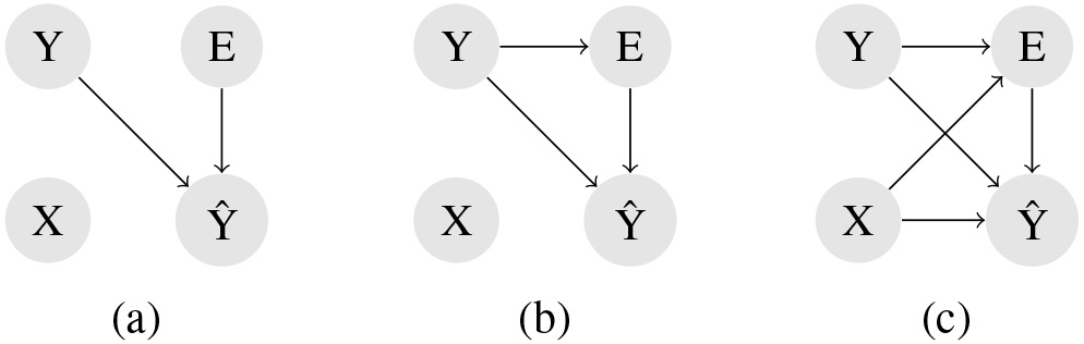

(1)

Noisy Completely at Random (NCAR): the occurrence of a mislabeled instance is independent of the instance’s attributes and class. Mislabeled records are uniformly present across the instance space. In a binary classification problem, for example, there will exist the same proportion of mislabeled instances in both classes. In other words, as shown in Fig. 1a, the occurrence of an error E is independent of the other random variables, including the true class itself (Y). For this model, the mislabeled instance probability is given by $p_{e}=P(E=1)=P(Y\neq\textit{\^{Y}})$ .

(2)

Noisy at Random (NAR): the labeling errors probability depends on the instance class, although it is not dependent on records’ attributes. Once mislabeling is conditional to instance classes, it allows us to model asymmetric label noise, i.e., when samples from certain classes are more prone to be mislabeled. This model could be applied, for example, to simulate mislabeling classification that is often verified in medical case-control studies where the misclassification of disease outcome may be unrelated to risk factor exposure (non-differential) [13]. As shown in Fig. 1b, E is still independent of X but it is conditioned by Y. For this model, the mislabeled instance probability is given by $p_{e}=P(E=1)=\sum_{y\in Y}P(Y=y)P(E=1|Y=y)$ .

(3)

Noisy not at Random (NNAR): the probability of an error occurrence depends not only on the instance class but also on the instance attributes. In this case, for example, samples are more likely to be mislabeled when they are similar to records of another class or when they are located in certain regions of the instance space. By applying this model, it is possible to simulate mislabeling near classification boundaries or in low-density regions. It also can be used for medical case-control studies where the misclassification of disease outcome may be related to risk factor exposure (differential) [13]. As can be seen in Fig. 1c, this is a more complex model, where E depends on both X and Y, i.e., labeling errors are more likely for certain classes and in certain regions of the X space.

It is usually quite challenging to identify the kind of noise present in a dataset without any background knowledge. Nevertheless, it is crucial to evaluate how sensitive noise detection techniques are to the noise distribution in a dataset. In this work, analyses regarding the NAR and NCAR models were performed in different contexts. NNAR scenarios are equally relevant, although more diverse in terms of assumptions that relate to the instances’ attributes and the chance of label noise. This work focused on the NAR and NCAR model to provide controlled experimental scenarios and investigate pertinent aspects (e.g., class distribution, noise level per class) that can impact label noise detection. Once deeply studied, such contexts can be extended in future work to cover the NNAR assumption.

2.3 Scope and contribution

As detailed previously, several works have extensively studied approaches to better handle noise detection either by developing noise-tolerant algorithms or by identifying and filtering data irregularities in a preprocessing step. In most previous studies, artificial noise is randomly injected into data to evaluate proposed systems. This work delivers relevant findings on how different noise models affect noise detection, indicating that new noise handlers systems should be evaluated in a broader context. In opposite to many related studies, which usually focus on creating new detectors, this paper analyses label noise detection under NCAR and NAR models and their behavior in different settings such as class imbalanced data, amount of noise, and noise distribution per class.

The current work is focused on evaluating ensemble filtering techniques, regarding different aspects that can impact the noise detection performance, such as the noise model, the class imbalance ratio and the noise level per class. Previous related works are commonly limited to evaluate ensemble filtering techniques assuming the NCAR model, such as [24, 14]. Differently, our work investigates the performance of noise filters under the NAR model, in which noise level can vary depending on the class. Additionally, we addressed other aspects like class imbalance ratio and noise level per class, to investigate the impact on noise detection performance, also depending on the noise model assumed in the experiments.

Previous works on ensemble noise filtering are also limited to evaluate and selecting between the majority or the consensus approach. The trade-off between choosing the majority or the consensus approach can be replaced by the problem of choosing a vote threshold. The majority and the consensus are special cases, when thresholds are 50% and 100%, respectively. The adequate vote threshold would be related to the expected proportion of noisy instances in a dataset. Nevertheless, few works have investigated the influence of varying the vote thresholds. For instance, in [17, 21], the authors showed that selecting adequate values of the vote threshold usually performed better than using the standard filtering approaches. The choice of the vote threshold is another important aspect that is addressed in the current work.

As it will be seen, our work produced important findings which can be considered when developing new noise detection techniques, evaluating existing approaches, and modeling specific real-world problems.

3. Proposed methodology

This section details the experimental setup adopted in our work to evaluate the ensemble noise detectors under NCAR and NAR models. Different aspects are jointly considered in the performed evaluation, which were not properly evaluated yet in the literature: (1) the class imbalance ratio in a dataset; (2) the noise ratio comparing the majority and minority classes; (3) the noise model itself.

The experimental protocol adopted in this work is summarized in Fig. 2. The protocol starts with a real-world dataset given as input. Initially, a data cleaning process using the consensus vote is applied to remove possible noise from the input dataset. Then a new dataset is generated from the cleaned data with the desired class imbalance ratio (IR). The generated dataset is split into training (70%) and testing (30%) data. The training data is used to produce the pool of classifiers used for ensemble noise detection.

Figure 2.

General experimental protocol.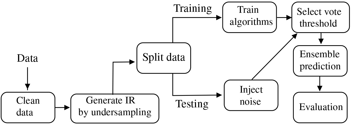

For evaluating the noise detector, the percentage of noise p is injected into the testing data according to the noise ratio M and a chosen noise model. Each test instance is given as input to the pool of classifiers. With all predictions, the test instance is marked as noisy if at least L classifiers misclassify it. Then, some evaluation measures described in this section are calculated and analyzed.

The main purpose of the proposed methodology of experiments is to derive insights on how to design ensemble noise detectors under specific conditions, like different class distributions and noise levels per class. It is important to highlight that domain knowledge and experts (when available) can be very helpful to estimate such specific conditions. For instance the noise level per class can be estimated by relying on an expert inspection of a sample of data instances to identify eventual labeling errors. Once such conditions are identified via auxiliary data and experts, the design of the noise detectors can be more adequately performed.

In Section 3.1, the algorithms for the ensemble filter and the vote scheme approach are presented. In Section 3.2, the real-world datasets are detailed, and it is described the methodology for data generation with specific settings. The procedure for noise injection regarding the noise model is explained in Section 3.3. Depending on the label noise model adopted in the experiments, noise detection techniques can have distinct performance behavior, usually measured by precision and recall, defined in Section 3.4. Lastly, the input variables and the experimental protocol are summarized in Section 3.5.

3.1 Ensemble

The noise detection ensemble used in the experiments was generated from 10 algorithms adopted in the related work [24]. They were chosen from different families: decision trees, Bayesian models, neural networks, support vector machines, random forest, nearest neighbors, and ruled-based methods, forming a diverse pool of classifiers. All of them are implemented in R from specific packages, as shown in Table 1. Default parameters suggested in the R packages were employed for all algorithms in the experiments. Parameters could be optimized for each algorithm, which would result in more accurate classifiers. However, as we are dealing with ensembles, the lack of parameter optimization would be compensated by using diverse algorithms. The impact of parameter optimization in ensemble noise detection will be better investigated in future work.

Table 1
Learning algorithms for classification noise filtering

Algorithm	R package
CN2 (rule learner)	RoughSets
kNN (nearest neighbor)	Class
Naive Bayes	Naivebayes
Random forest	RandomForest
SVM (RBF Kernel)	e1071
J48	RWeka
JRip	RWeka
Multiplayer perceptron	RSNNS
Decision tree	Party
SMO (linear Kernel)	RWeka

Unlike previous work that adopted the majority and the consensus vote approaches for ensemble-based noise filtering, in our work, we evaluate different values for the decision threshold L in the ensemble. If more than L% of classifiers in the pool misclassify an instance, it is considered wrongly labeled. In our experiments, the threshold L varies from 10% to 100%. The majority and the consensus approaches are special cases, respectively, assuming L $=$ 50% (i.e., more than half classifiers plus 1) and 100% (i.e., all classifiers). Of course, too small values, like 10%, would be reasonable only in contexts with almost noise-free datasets and/or ones that want to force a very high level of recall in noise detection. Nevertheless, we vary L to check if there is a threshold that maximizes the noise detection under specific contexts, i.e., considering the class imbalance ratio, noise distribution, and percentage of total noise.

3.2 Data

Quantitative assessment of noise detection methods requires knowing which are the noisy instances beforehand. In real-world datasets, this is achieved either by expert labeling or by randomly injecting artificial noise into a dataset. While the former approach is not feasible for an extensive evaluation, the latter still has uncertainty about which instances are originally noisy when dealing with real-world datasets.

Table 2
Real-world data information. Missing $=$ instances with at least one missing value

Dataset	Attr.	Original			After cleaning
		IR	Inst.	Missing	IR	Inst.	Removal (%)
Arcene	10001	44:56	200	0	44:56	199	0.50
Breast-c	10	34:66	699	16	35:65	673	3.72
Column2C	7	32:68	310	0	32:68	308	0.65
Credit	16	44:56	690	37	45:55	644	6.67
Cylinder-bands	40	42:58	540	263	36:64	276	48.89
Diabetes	9	35:65	768	0	31:69	720	6.25
Eeg-eye-state	15	45:55	14980	0	45:55	14979	0.01
Glass0	10	33:67	214	0	33:67	214	0.00
Glass1	10	36:64	214	0	35:65	212	0.93
Heart-c	14	46:54	303	7	45:55	289	4.62
Heart-statlog	14	44:56	270	0	44:56	262	2.96
Hill-valley	101	50:50	1212	0	48:52	1184	2.31
Ionosphere	35	36:64	351	0	35:65	345	1.71
Kr-vs-kp	37	48:52	3196	0	48:52	3194	0.06
Mushroom	23	48:52	8124	2480	38:62	5644	30.53
Pima	9	35:65	768	0	32:68	732	4.69
Sonar	61	47:53	208	0	46:54	206	0.96
Steel-plates-fault	34	35:65	1941	0	35:65	1941	0.00
Tic-tac-toe	10	35:65	958	0	35:65	958	0.00
Voting	17	39:61	435	203	47:53	228	47.59

In our experiments, we adopted 20 real-world binary datasets available at the KEEL-dataset repository [2], UCI repository [8], and Open Media Library [27]. Some multi-class datasets are modified to obtain two-class imbalanced problems, defining the joint of one or more classes as positive and the remainder as negative. The list of datasets is presented in Table 2.

Figure 3.

Data generation process.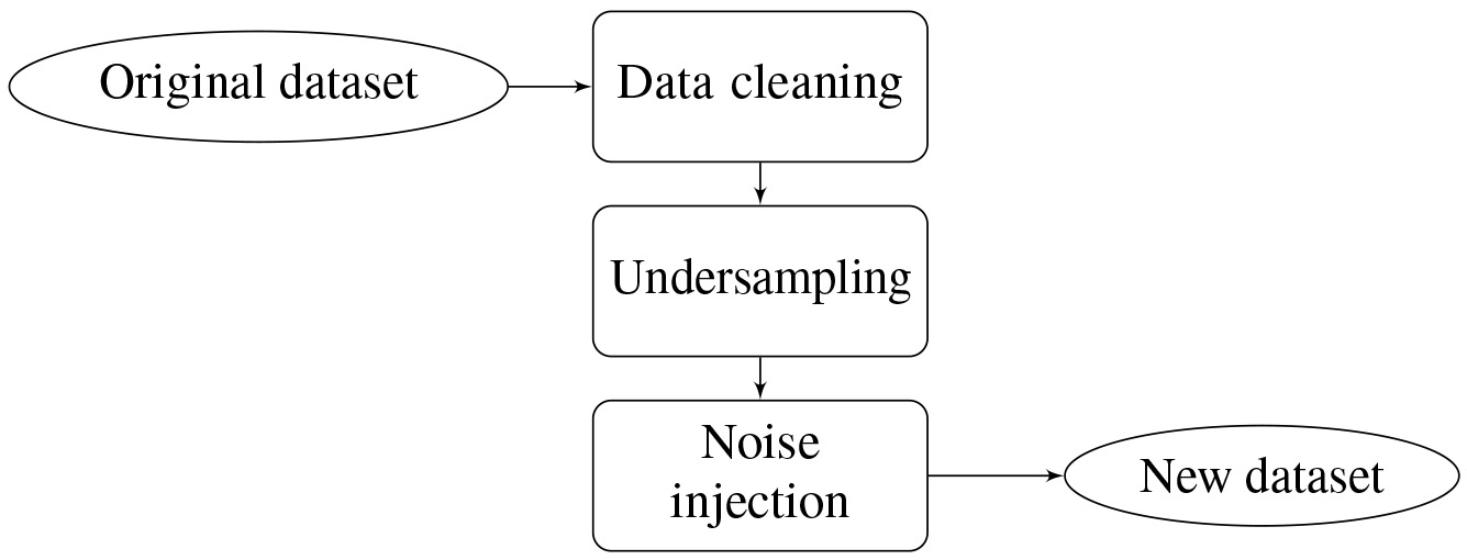

For each dataset, a three-step process is adopted (see Fig. 3) to generate a new dataset with controlled IR and injected label noise. The dataset generation process is described below:

•

Data cleaning: As suggested in [24], a data cleaning step is applied to reduce the inherent label noise that is possibly present in the dataset. Hence, the evaluation of noise detection will be mainly contingent on the artificial noise injected in a controlled manner. In this step, a 10-fold classification is employed, and the consensus method is used to remove noisy instances. The consensus vote was chosen for this step for being more strict, ensuring that only instances undoubtedly noisy are discarded since it requires all ensemble classifiers’ agreement.

•

Undersampling: In this step, three datasets are generated for each cleaned data, in order to obtain the following IR configurations: (1) 50:50, (2) 30:70, and (3) 20:80. For generating a dataset with a given IR, a random undersampling process of the majority class is applied.

•

Noise injection: In this step, noise is artificially injected according to a given label noise model. This step is detailed in Section 3.3.

3.3 Noise injection

For noise detection evaluation, label noise is injected into the test set by changing the class label in a determined proportion $p$ of records. In our experiments, the desired noise level p assumed four different values: 5%, 10%, 15%, and 20% of instances.

For the NAR model, the noise is inserted to achieve a specific ratio $M$ of noisy instances per class. Two values of $M$ were chosen in such a way to analyze the impact of a significant discrepancy in the noise level per class:

•
$M=$ 9/1: for every nine noisy instances in the minority class, there is one noisy instance in the majority class. It simulates a scenario of application in which it is more difficult to label examples in the minority class. This chosen ratio is referred to as NAR (9:1) in the discussion of results.
•
$M=$ 1/9: in turn, for each noisy instance in the minority class, there are nine noisy instances in the majority class. It means that the majority class is more prone to have label noise. This chosen ratio corresponds to NAR (1:9) in the discussion of results.

Notice that the NCAR model is a particular case of NAR by assuming $M=$ 1, i.e., NCAR is equivalent to NAR (1:1).

Each class’s exact number of noisy instances is determined according to the desired noise level $p$ and the ratio $M$ . Let $d_{n}$ be the number of instances in the test set. Let $n_{1}$ and $n_{2}$ be the number of noisy instances in each class. Then $n_{1}+n_{2}=p\times d_{n}$ and $M=n_{1}/n_{2}$ . In order to obtain such constraints, $n_{1}$ and $n_{2}$ are defined according to the following equations:

$\displaystyle n_{1}=\frac{M\times(d_{n}\times p)}{M+1}$ (1) $\displaystyle n_{2}=\frac{d_{n}\times p}{M+1}$ (2)

For example, suppose that we have $d_{n}=$ 1000 records in the test set, and the desired noise level is $p=$ 0.10 (100 noisy instances). Then, consider that noise is injected according to the three settings: NCAR, NAR (9:1) NAR (1:9). In the first setting, $M=$ 1, and by adopting the above equations, we would find $n_{1}=$ 50 and $n_{2}=$ 50. The number of noisy instances in the test set is the same for both classes. This example is illustrated in Fig. 4.

Figure 4.
Noise injection with NCAR model for different imbalance ratios (IR).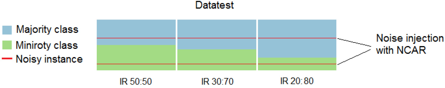

In the NAR (9:1) setting, $M=$ 9 and then $n_{1}=$ 90 (90 noisy instances in minority class) and $n_{2}=$ 10 (10 noisy instances in majority class). In this case, the noise level in minority class is higher in the test set. This example is illustrated in Fig. 5.

Table 3
Experimental setup

Imbalance Ratio (IR) Total percentage of Noise Ratio (M)

Class min: Class maj noise in testing set (p) Class min: Class maj

50:50 5% 10% 15% 20% NCAR

NAR (1:9)

NAR (9 : 1)

30:70 5% 10% 15% 20% NCAR

NAR (1 : 9)

NAR (9 : 1)

20:80 5% 10% 15% 20% NCAR

NAR (1:9)

NAR (9 : 1)

Figure 5.
Noise injection with NAR 9:1 model for different imbalance ratios (IR).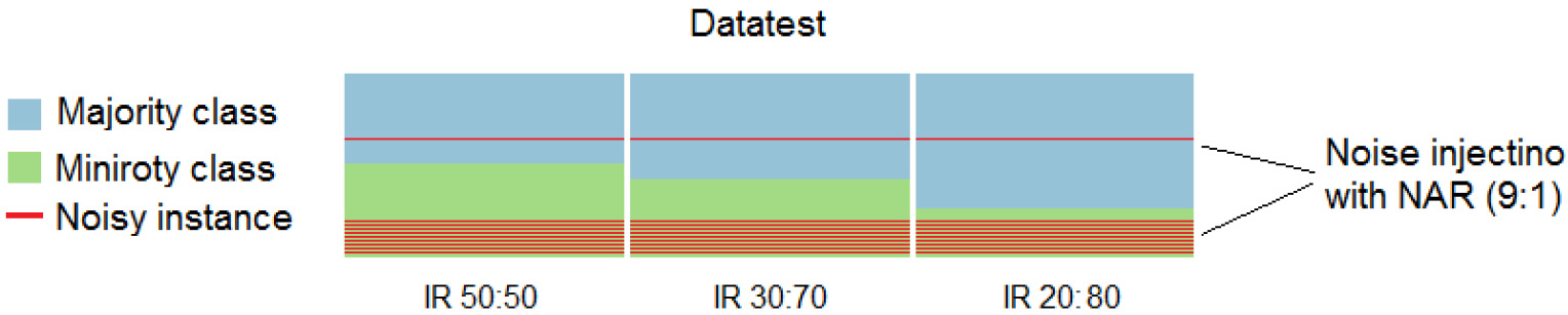

Finally, for the NAR (1:9) setting, $M=$ 1/9, hence, $n_{1}=$ 10 (10 noisy instances in the minority class) and $n_{2}=$ 90 (90 noisy instances in the majority class). In this case, the number of noisy instances injected in the test set is greater for the majority class, as illustrated in Fig. 6.

Figure 6.
Noise injection with NAR 1:9 model for different imbalance ratios (IR).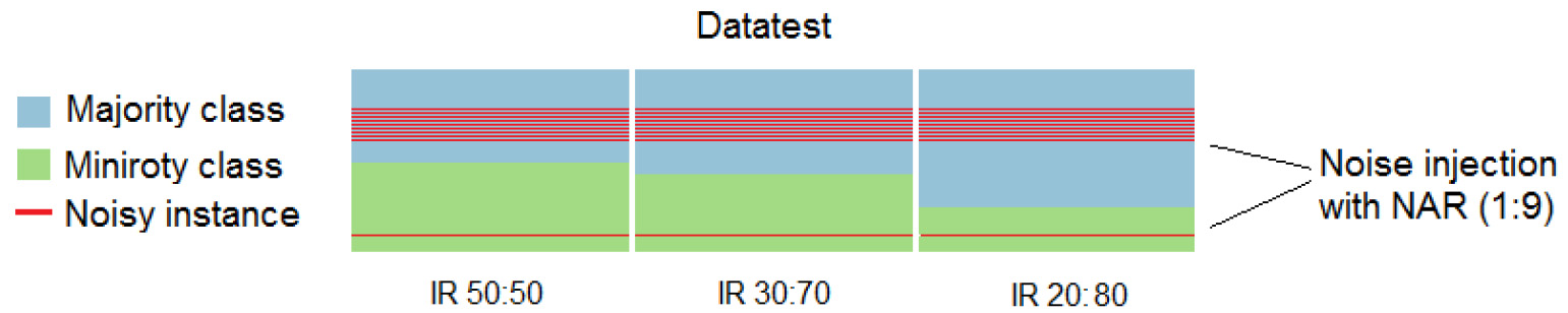

3.4 Performance measures

Most experiments in the literature assess the efficiency of methods in detecting noise regarding accuracy [9]. A primary measure to evaluate the performance of noise detection is precision, which means how many noisy instances the detector correctly identified among all records identified as noisy:

$\displaystyle\text{Precision}=\frac{\text{number of noisy cases correctly % identified}}{\text{number of all noisy cases identified}}$

In addition to the precision, another helpful measure is recall, which calculates how many instances the detector correctly identified as noisy among all the noisy records inserted into the dataset:

$\displaystyle\text{Recall}=\frac{\text{number of noisy cases correctly % identified}}{\text{number of all noisy cases in dataset}}$

Finally, a measure that trades off precision versus recall is the F-score, which is the weighted harmonic mean of precision and recall:

$\displaystyle\textit{F-score}=\frac{\beta\times\textit{Precision}\times\textit% {Recall}}{\textit{Precision}+\textit{Recall}}$ (3)

where $\beta^{2}=\frac{1-\alpha}{\alpha}$ , with $\alpha\in[0,1]$ and $\beta^{2}\in[0,\infty]$ .

Setting the $\beta$ parameter makes it possible to assign more importance to either precision or recall when calculating the F-score. In this work, the standard F-score (also referred to as $F_{1}\textit{score}$ , $\beta=$ 1 and $\alpha=$ 1/2) was used. It equally weights precision and recall.

3.5 Experimental protocol algorithm

The experimental protocol illustrated in Fig. 2 is also outlined in Algorithm 1. The algorithm was executed for each input parameter combination shown in Table 3. Given the stochastic nature of noise injection, this insertion is usually repeated several times for each noise level [23, 32]. In this work, for each parameters combination, Algorithm 1 was repeated 100 times, and the average results of Precision, Recall, and F1-Measure were employed to evaluate the ensemble noise detector.

Algorithm 1: Experimental procedure
Input: IR, M, p, dataset, classifiers, threshold (L)
Output: performance measures
1: cleanData $\leftarrow$ dataCleasing(dataset, classifiers)
2: data $\leftarrow$ generateData(cleanData, IR)
3: training, testing $\leftarrow$ split(data, 70%; 30%) {Split data in training and testing data}
4: noisy_testing $\leftarrow$ injectNoise(testing, M; p)
5: for c in classifiers do
6: model $\leftarrow$ train(training, c)
7: predictions $\leftarrow$ classify(model, noisy_testing)
8: end for
9: ensemble_prediction $\leftarrow$ voting(predictions; L)
10: measures $\leftarrow$ calculate(ensemble_prediction)

4. Results

In this section, the findings from the experiments described in Section 3.5 are presented and examined. The results shown in this section were obtained from the steps outlined in Algorithm 1. The discussion is carried out by putting into perspective each input parameter that resulted in a specific scenario, facilitating the analysis and comparison. In this way, we first examine the noise detection concerning balanced and imbalanced datasets exploring the impact of different noise levels per class in Section 4.1. In Section 4.2, we analyze noise detection under different noise ensemble thresholds. Lastly, statistical tests of the results are detailed in Section 4.3.

4.1 Imbalance ratio and noise level per class

Figures 7 and 8 show the F-score for eight datasets, varying the noise level and the imbalance ratio. F-score tends to increase as the general noise level (p) increases as well. Similar patterns of results were observed in the other datasets. This is expected since the noise detection task becomes easier for higher amounts of noise in a dataset.

The general behavior observed in the scenario of balanced data (IR 50:50 – first column) was that NCAR and NAR models produced the same effect on noise detection regardless of the noise distribution (noise level per class). In other terms, when the dataset is balanced, the noise detection performance depends more on the percentage of noise in the dataset than on how the noise is distributed per class.

For imbalanced datasets, noise detection is affected by the noise level per class, as revealed by the F-score discrepancy between NCAR and NAR models shown in Figs 7 and 8. This difference increases when the noise level gets higher, as observed for arcene and cylinder-bands datasets in a more pronounced way. Smaller differences in NCAR and NAR models results were mainly observed when the noise level was 5%. In such a noise level, it is, in fact, more difficult to obtain good performance measures.

Figure 7.

F-score performance for majority vote on arcene, cylinder-bands, diabetes, and eeg-eye-state datasets.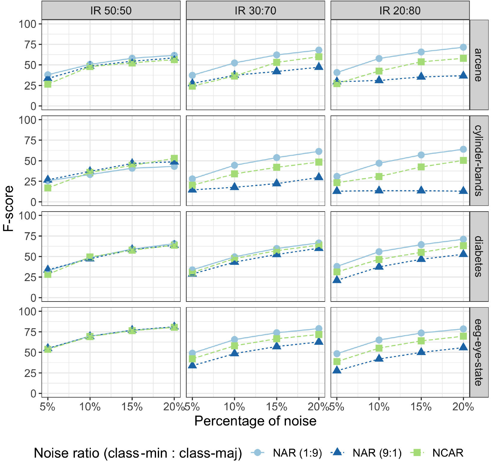

Figure 8.

F-score performance for majority vote on heart-c, heart-statlog, hill-valley, and pima datasets.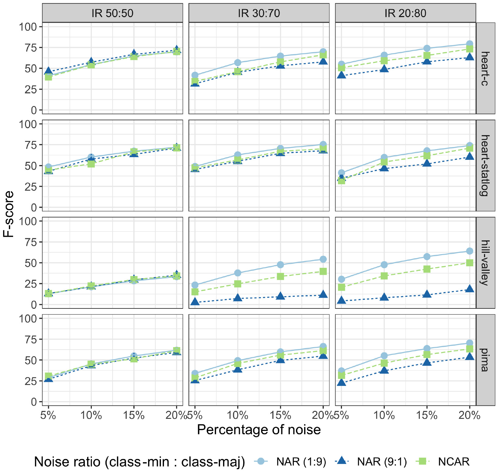

Table 4

F-score variation vs class imbalance ratio

Datasets	F-score variation when IR goes from 50:50 to 20:80
	5% of noise						10% of noise						15% of noise						20% of noise
	NAR (9:1)		NCAR		NAR (1:9)		NAR (9:1)		NCAR		NAR (1:9)		NAR (9:1)		NCAR		NAR (1:9)		NAR (9:1)		NCAR		NAR (1:9)
Arcene	$-$ 3.	6	1.	1	2.	8	$-$ 17.	4	$-$ 5.	4	7.	1	$-$ 19.	2	1.	3	7.	6	$-$ 21.	6	1.	7	9.	8
Breast-cancer-wisconsin	$-$ 1.	1	$-$ 1.	4	4.	7	$-$ 0.	4	0.	0	3.	8	$-$ 0.	9	$-$ 0.	6	2.	2	$-$ 0.	4	$-$ 0.	1	1.	7
Column2C	$-$ 13.	6	4.	1	$-$ 2.	8	$-$ 10.	5	$-$ 2.	1	$-$ 0.	4	$-$ 15.	6	1.	7	1.	8	$-$ 13.	3	$-$ 2.	4	0.	9
Credit	$-$ 5.	8	$-$ 1.	2	2.	3	$-$ 8.	6	0.	6	1.	6	$-$ 7.	0	0.	0	1.	4	$-$ 6.	6	$-$ 0.	3	2.	0
Cylinder-bands	$-$ 13.	8	6.	6	5.	4	$-$ 23.	6	$-$ 5.	1	13.	8	$-$ 33.	0	$-$ 1.	8	16.	2	$-$ 35.	8	$-$ 2.	6	20.	8
Diabetes	$-$ 12.	8	3.	0	5.	5	$-$ 10.	0	$-$ 2.	9	7.	2	$-$ 11.	8	$-$ 2.	6	5.	4	$-$ 11.	1	$-$ 0.	6	5.	4
Eeg-eye-state	$-$ 27.	2	$-$ 15.	0	$-$ 6.	3	$-$ 27.	5	$-$ 14.	0	$-$ 4.	8	$-$ 27.	0	$-$ 12.	4	$-$ 3.	4	$-$ 25.	4	$-$ 10.	9	$-$ 2.	2
Glass0	$-$ 1.	5	1.	9	$-$ 3.	0	$-$ 0.	5	8.	8	7.	9	$-$ 5.	1	3.	5	6.	5	$-$ 4.	5	3.	3	8.	9
Glass1	$-$ 7.	6	$-$ 6.	2	$-$ 0.	8	$-$ 18.	1	3.	1	8.	8	$-$ 21.	6	2.	2	8.	9	$-$ 27.	0	$-$ 1.	8	11.	9
Heart-c	$-$ 4.	7	11.	1	13.	7	$-$ 8.	8	4.	9	11.	4	$-$ 9.	0	1.	3	9.	2	$-$ 8.	8	3.	1	9.	6
Heart-statlog	$-$ 8.	2	$-$ 12.	6	$-$ 7.	0	$-$ 11.	4	2.	3	$-$ 0.	5	$-$ 11.	4	$-$ 4.	6	0.	4	$-$ 10.	9	$-$ 0.	3	2.	1
Hill-valley	$-$ 8.	8	7.	6	17.	4	$-$ 13.	3	12.	1	26.	5	$-$ 18.	1	12.	6	29.	0	$-$ 17.	2	15.	7	30.	8
Ionosphere	$-$ 4.	6	$-$ 5.	3	3.	6	$-$ 4.	1	$-$ 2.	8	3.	3	$-$ 6.	4	1.	5	1.	1	$-$ 4.	7	0.	1	1.	9
Kr-vs-kp	$-$ 8.	7	$-$ 6.	8	$-$ 7.	4	$-$ 5.	9	$-$ 3.	9	$-$ 3.	6	$-$ 4.	7	$-$ 3.	0	$-$ 3.	0	$-$ 3.	9	$-$ 2.	1	$-$ 2.	0
Mushroom	$-$ 0.	1	$-$ 0.	1	$-$ 0.	1	$-$ 0.	0	$-$ 0.	0	$-$ 0.	1	$-$ 0.	0	$-$ 0.	0	$-$ 0.	0	$-$ 0.	0	$-$ 0.	0	$-$ 0.	0
Pima	$-$ 4.	5	0.	9	8.	2	$-$ 6.	1	1.	4	9.	9	$-$ 5.	9	5.	0	8.	9	$-$ 5.	7	2.	3	8.	5
Sonar	14.	1	18.	6	15.	0	13.	4	13.	4	19.	4	9.	0	13.	7	17.	8	6.	3	10.	0	16.	5
Steel-plates-fault	0.	0	1.	0	0.	4	$-$ 0.	0	0.	4	0.	3	0.	0	0.	4	0.	2	$-$ 0.	0	0.	1	0.	1
Tic-tac-toe	$-$ 22.	1	$-$ 4.	9	5.	0	$-$ 26.	1	$-$ 5.	9	5.	4	$-$ 26.	6	$-$ 5.	2	5.	1	$-$ 27.	1	$-$ 5.	4	5.	4
Voting	$-$ 6.	8	$-$ 13.	6	$-$ 4.	1	$-$ 5.	8	$-$ 7.	6	$-$ 2.	5	$-$ 4.	4	$-$ 6.	2	$-$ 2.	0	$-$ 4.	7	$-$ 4.	8	$-$ 1.	4

Table 4 shows how F-score changes when the scenario varies from a balanced dataset to an imbalanced dataset. Negative and positive numbers denote, respectively, a decrease and increase in noise detection. As can be seen, noise distribution is important when considered in combination with class imbalance. For instance, under the NAR (9:1) model (i.e., more noise instances in the minority class than in the majority’s), noise detection worsened its performance when class imbalance was increased. This was the overall behavior confirmed by the negative F-score variation presented in Table 4 at NAR (9:1) column. On the other hand, an opposite pattern of results was observed for the NAR (1:9) model, i.e., noise detection was improved when class imbalance increased. The greater number of positive F-score variations found at the NAR (1:9) column endorse that, in imbalanced datasets, noisy instances in the majority class tend to be more easily detected than noisy instances in the minority class. No consistent pattern of performance was observed in Table 4 for the NCAR model. This indicates that when the noise is evenly distributed in an imbalanced dataset, the particularities and difficulties of the problem itself may be more crucial in noise detection performance than the IR.

Noise detection was impacted by class imbalance under the NAR model as expected. For a better visualization of this result, Figs 9 and 10 show the general behavior of noise detection under the NAR model when IR increases. This can be observed by the more prominent and negative bar on the left side of the graphs in contrast to a smaller and positive bar on the right. This comportment was observed in all datasets, except for the sonar dataset. This may imply that the noise model characteristics and class imbalance ratio, in general, have more influence on noise detection than the nature of the classification problem for the majority of problems.

Figure 9.

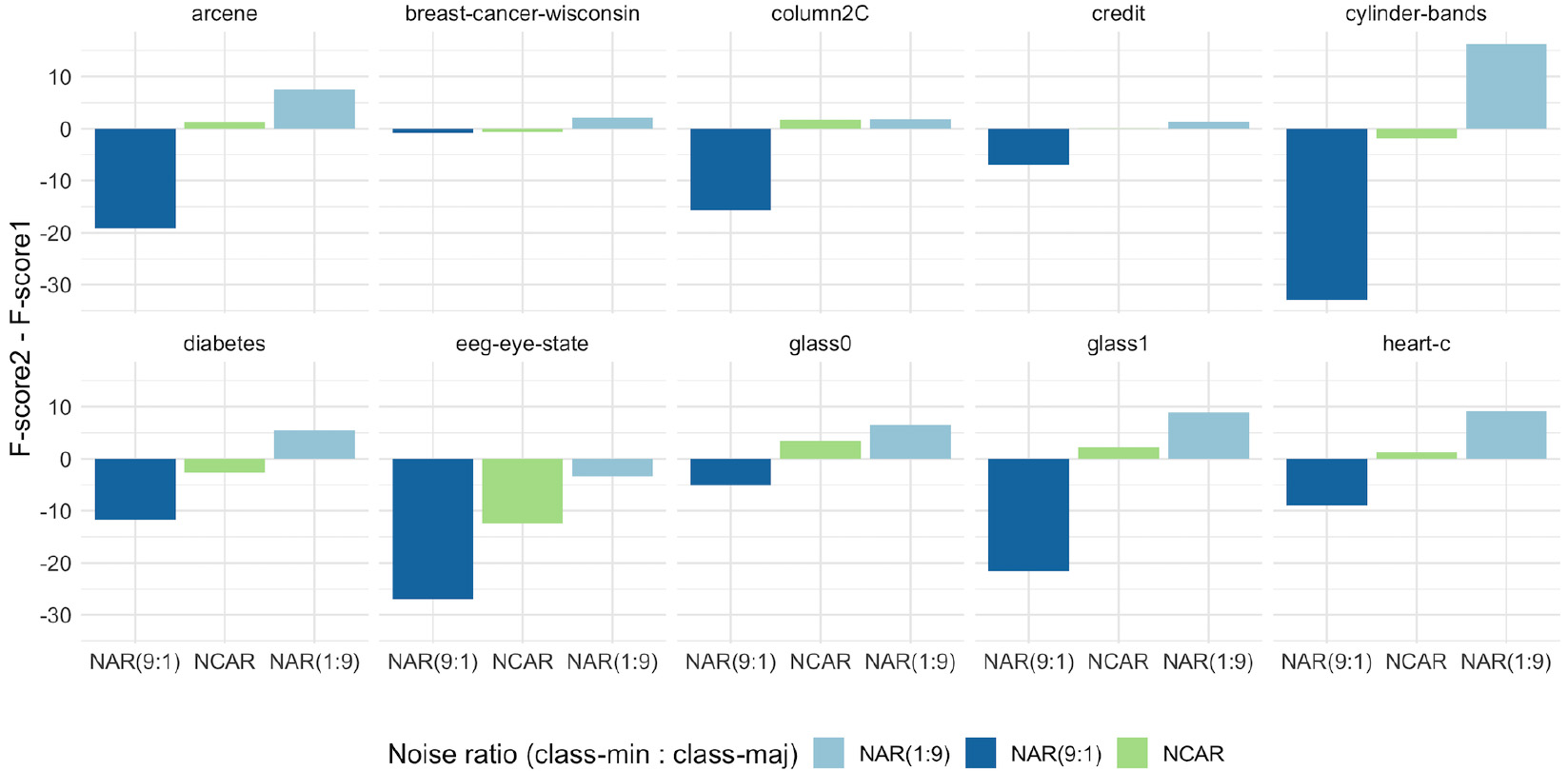
Variation in F-score performance when IR increases from 50:50 (F-score1) to 20:80 (F-score2) in presence of a noise level of 15%.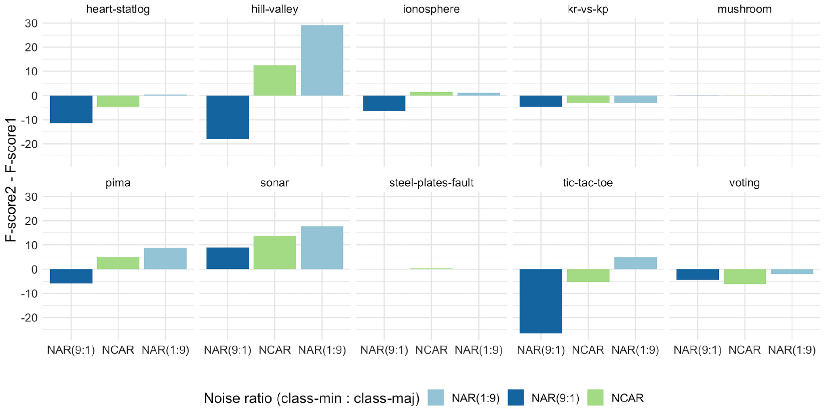

Figure 10.

Variation in F-score performance when IR increases from 50:50 (F-score1) to 20:80 (F-score2) in presence of a noise level of 15%.

4.2 Noise detection vs ensemble vote thresholds

Figures 11 and 12 show the noise detection performance under different ensemble vote thresholds for each dataset at 15% of noise level for the NAR and NCAR models.

As can be seen, for most datasets, similar behavior was observed: better noise detection was achieved with smaller threshold values under the NAR (9:1) model (i.e., more noise instances in the minority class than in the majority’s), and higher threshold values under the NAR (1:9) model when IR is increased. Under the NCAR model, threshold values close to $L=$ 5 (majority vote) returned higher F-score results.

The above behavior is verified in a more or less pronounced way depending on the dataset. For example, in Fig. 11 for arcene dataset, the best threshold under the NAR(9:1) model is $L=$ 7 when IR is 50:50, $L=$ 5 when IR is 30:70, and $L=$ 3 for an IR of 20:80. Under the same settings, for pima dataset in Fig. 12, the best threshold under the NAR(9:1) model is $L=$ 8 when IR is 50:50, $L=$ 6 when IR is 30:70 and $L=$ 4 for an IR of 20:80. The optimal values for each dataset are different, but the general behavior is the same. When varying the ensemble threshold, experiments show that a smaller number of voter algorithms delivers better noise detection under NAR(9:1) model, and that a greater threshold produces better performance under NAR(1:9). Finally, under NCAR models, the majority vote performs better.

Our results imply a change in the common practice adopted in the literature. The majority vote detection, widely used in related studies, corresponds to applying a default decision threshold. This is not the best option if it is expected a different noise level per class. Better thresholds can be set to improve noise detection performance. Different aspects like the class imbalance ratio and the noise model have to be considered.

4.3 Statistical tests

The Friedman test [10] was performed in order to compare the impact of all three noise models over the 228 problems (19 datasets1

¹
Mushroom dataset was removed because of its 100% precision.

\times

3 IR’s

\times

4 different percentages of noise). The level of significance was set to

\alpha=

0.05, i.e., 95% confidence.

The Friedman test shows a significant difference in the detection noise for the three models in certain contexts. As shown in Table 5, from the 152 data imbalanced problems analyzed, 77.63% (118/152) presented a significant difference in the detection results. When considering only the problems with 20:80 IR, this number is equal to 88.16%. On the other hand, when it comes to balanced datasets (76 of cases), only 18.42% are significantly different. These results are aligned with the hypothesis discussed in the previous section. The choice of a noise generation model is more likely to impact detection results in data-imbalance problems.

The influence of the amount of noise on ensemble detection was also tested. From the 57 problems for each percentage of noise, approximately half of the cases presented a significant difference (56.1% for 5% of noise, 54.4% for 10%, 63.2% for 15% and 57.9% for 20%). In this way, the amount of noise in data seems not to be as relevant as the IR on noise detection under different noise models.

A second statistical analysis was also conducted in a pairwise fashion in order to verify if the noise models significantly improved/harmed the noise detection under certain contexts. In order to do so, the Wilcoxon non-parametric signed-rank test with the level of significance $\alpha=$ 0.05 was used in all problems.

Table 5

Summary of Friedman test results on each problem

IR	Cases with significant difference								Total per IR
	5% of noise		10% of noise		15% of noise		20% of noise
50:50	6/19	31.6%	1/19	5.3%	6/19	31.6%	1/19	5.3%	14/76	18.4%
30:70	11/19	57.9%	14/19	73.7%	12/19	63.2%	14/19	73.7%	51/76	67.1%
20:80	15/19	78.9%	16/19	84.2%	18/19	94.7%	18/19	94.7%	67/76	88.2%
Total	32/57	56.1%	31/57	54.4%	36/57	63.2%	33/57	57.9%

Figure 11.

F-score on arcene, cylinder-bands, diabetes, and eeg-eye-state datasets under different ensemble vote thresholds (where 1 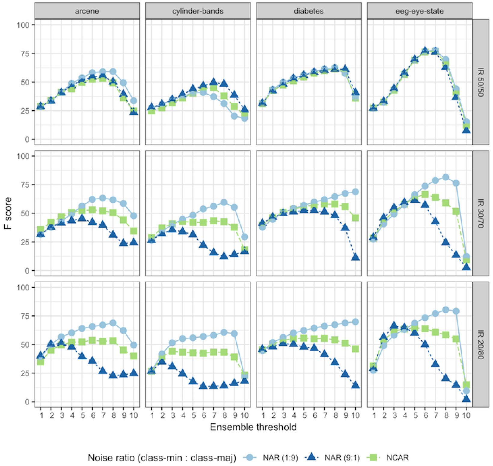$=$ 10%, 2 $=$ 20%, $\ldots$ , 10 $=$ 100%) in presence of 15% of noise.

Figure 12.

F-score on heart-c, heart-statlog, hill-valley, and pima datasets under different ensemble vote thresholds (where 1 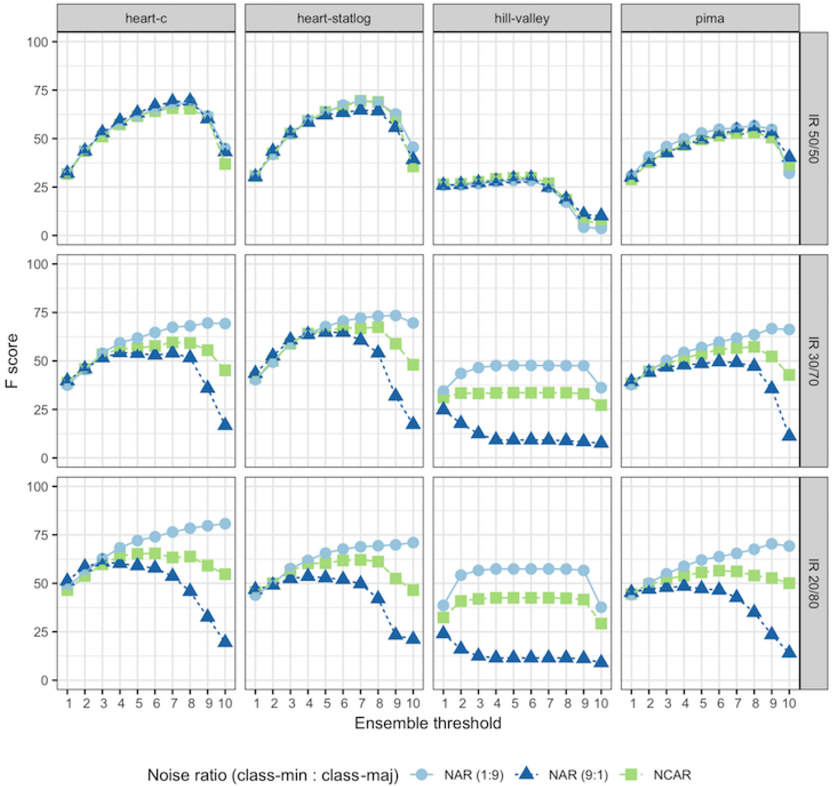$=$ 10%, 2 $=$ 20%, $\ldots$ ,10 $=$ 100%) in presence of 15% of noise.

The tests were performed for each percentage of noise. As the results were equivalent (independently of the amount of noise), the following discussion will be regarding the noise percentage of 15% shown in Table 6.

Table 6 presents a pairwise comparison of noise detection results for each noise model. The W/T/L denote the wins (better performance on noise detection), ties (equivalent performance on noise detection), and losses (worse performance on noise detection) produced by the noise models on the columns in comparison to the ones on the rows. For instance, the ensemble detector on problems under NAR(1:9) with 30:70 IR (column) performed 4 times better and 15 times worse (4/0/15) in comparison to the detection on problems under NAR(1:9) with 50:50 IR (row). For this same example, the p-value $=$ 0.007 implies there is a significant difference in the results.

Focusing on problems under the same IR, only one case showed a significant difference, as discussed previously. For balanced data, the NAR(1:9) model (more noise in the majority class) produced a positive impact on noise detection, performing 15 times out of 19 better than the detection under NCAR, although with a p-value $=$ 0.038. For the case of 30:70 IR, the NAR(9:1) model (more noise in the minority class) harmed detection as its performance was worse 17 times when compared to the detection under NCAR and NAR(1:9) models with a really small p-value. This was also verified when data was exposed to a different percentage of noise. Lastly, when increasing IR (20:80), tests showed noise detection is significantly improved under NAR(1:9) in comparison to the other noise models as the ensemble detector performed better in all problems (19/0/0).

Table 6

Wilcoxon test on real problems when there is 15% noise in data. W \T \L $=$ wins\ties\losses. $p$ -value $<$ 0.05 are highlighted

IR	Noise model		50:50		30:70			20:80
			NCAR	NAR (1:9)	NAR (9:1)	NCAR	NAR (1:9)	NAR (9:1)	NCAR	NAR (1:9)
50:50	NAR(9:1)	W/T/L	5/0/14	11/1/7	16/0/3	17/0/2	15/0/4	17/0/2	17/0/2	16/0/3
		$p$ -value	0.073	0.360	0.001	0.000	0.001	0.001	0.001	0.001
	NCAR	W/T/L		15/0/4	11/0/8	10/0/9	9/0/10	13/0/6	8/0/11	12/0/7
		$p$ -value		0.038	0.481	0.952	0.324	0.409	0.952	0.153
	NAR(1:9)	W/T/L			6/0/13	4/0/15	4/0/15	3/0/16	3/0/16	3/0/16
		$p$ -value			0.021	0.005	0.007	0.003	0.002	0.004
30:70	NAR(9:1)	W/T/L				17/0/2	17/0/2	16/0/3	16/0/3	17/0/2
		$p$ -value				0.000	0.000	0.012	0.001	0.000
	NCAR	W/T/L					17/0/2	4/0/15	9/0/10	15/0/4
		$p$ -value					0.000	0.004	0.856	0.004
	NAR(1:9)	W/T/L						1/0/18	4/0/15	7/0/12
		$p$ -value						0.000	0.001	0.035
20:80	NAR(9:1)	W/T/L							18/0/1	19/0/0
		$p$ -value							0.000	0.000
	NCAR	W/T/L								19/0/0
		$p$ -value								0.000

5. Conclusions

Many studies have focused their attention on data quality issues due to its importance in ML applications and the known fact that real-world datasets frequently contain noise [9].

Noise can be presented in data in its attributes and also in its classes [31]. This work focused the studies on class noise (also label noise). For this type of problem, the classification noise filtering approach is usually applied to remove data irregularities before the learning step. The most common filtering consists of using the predictions of an ensemble of algorithms so that instances are removed upon a wrong classification [7, 24, 14].

To evaluate Noise Filters, simulated noise is usually injected into a dataset, and then analyses can be performed on the results [11]. In [9], three different label noise generation for injecting noise are presented: (1) NCAR, in which the probability of an instance being noisy is random, (2) NAR, the probability of an instance being noisy depends on its label, and (3) NNAR, the probability of an instance being noisy also depends on its attributes.

Although there are many approaches to model different noise behaviors, in many previous works [24, 7, 22, 11], one type of noise is chosen over another without considering the different impacts of each. Also, despite the majority and consensus vote approaches being the most common ensemble voting schemes used for filtering noise, studies [17, 21] have shown that selecting adequate values for the ensemble threshold can lead to superior results.

This work presented an empirical study focused on ensemble-based noise detection and its performance under three different noise models generation: NCAR, where noise is equally distributed among class, NAR model by applying more noise in the majority class, and NAR model by employing more noise in the minority classes. The relation between detection performance and injected noise model was assessed through performance measures (F-score, Precision, Recall), considering different ratios of inserted noise and imbalance class configurations. The impact produced on filtering performance was also evaluated under different ensemble thresholds.

As conclusions, we could observe that noise detection was not affected by the noise model in balanced data. In contrast, when dealing with imbalanced data, we faced two different scenarios for noise detection under the NAR model. Firstly, the addition of noise in the minority class harmed the noise detection in all problems. Moreover, by applying more noise in the majority class, noise detection improved in most cases. Besides, increasing the IR from 30:70 to 20:80 resulted in an even worse noise detection when the minority class was the noisiest one, and the opposite was verified when the majority class had more noise.

The experiments performed with different ensemble thresholds showed that not always majority and consensus voting are the best options. Better noise detection was achieved for both models NCAR and NAR(9:1) if less than 50% of the algorithms were selected. On the other hand, better noise detection was achieved for NAR(1:9) if more than 50% of the algorithms were selected.

As future work, we intend to investigate the NNAR model and evaluate other noise filtering techniques, expanding the work to multi-class problems as well.

Footnotes

Acknowledgments

This research has been supported in part by the following Brazilian agencies: CAPES, CNPq and FACEPE.

References

Abellán

and Masegosa

A.R.

, Bagging decision trees on data sets with classification noise, In Link

and Prade

, editors, Foundations of Information and Knowledge Systems, Berlin, Heidelberg, 2010. Springer Berlin Heidelberg, pp. 248–265.

AlcalA-Fdez

Fernandez

Luengo

Derrac

GarcIa

Sanchez

and Herrera

, Keel data-mining software tool: Data set repository, integration of algorithms and experimental analysis framework, Journal of Multiple-Valued Logic and Soft Computing 17(2-3) (2011), 255–287.

Sluban

D.G.B.

and Lavra

, Advances in class noise detection, In European Conference on Artificial Intelligence, 2015, pp. 1105–1106.

Biggio

Nelson

and Laskov

, Support vector machines under adversarial label noise, In Hsu

C.-N.

and Lee

W.S.

, editors, Proceedings of the Asian Conference on Machine Learning, volume 20 of Proceedings of Machine Learning Research, South Garden Hotels and Resorts, Taoyuan, Taiwain, 14–15 Nov 2011. PMLR, pp. 97–112.

Bootkrajang

, A generalised label noise model for classification in the presence of annotation errors, Neurocomputing 192 (2016), 61–71. Advances in artificial neural networks, machine learning and computational intelligence.

Bootkrajang

and Kaban

, Learning kernel logistic regression in the presence of class label noise, Pattern Recognition 47(11) (2014), 3641–3655.

Brodley

C.E.

and Friedl

M.A.

, Identifying mislabeled training data, In Artifficial Intelligence Review, 1999, pp. 131–167s.

Dua

and Karra Taniskidou

, UCI machine learning repository, 2017.

Frenay

and Verleysen

, Classification in the presence of label noise: A survey, IEEE Transactions on Neural Networks and Learning Systems 25(5) (2014), 845–869.

10.

Friedman

J.H.

and Rafsky

L.C.

, Multivariate generalizations of the wald-wolfowitz and smirnov two-sample tests, Ann Statist 7(4) (1979), 697–717.

11.

Garcia

L.P.

Lehmann

de Carvalho

A.C.

and Lorena

A.C.

, New label noise injection methods for the evaluation of noise filters, Knowledge-Based Systems 163 (2019), 693–704.

12.

Garcia-Gil

Luengo

Garcia

and Herrera

, Enabling smart data: Noise filtering in big data classification, Information Sciences 479 (2019), 135–152.

13.

Gilbert

Martin

R.M.

Donovan

Lane

J.A.

Hamdy

Neal

D.E.

and Metcalfe

, Misclassification of outcome in caseâ€“control studies: Methods for sensitivity analysis, Statistical Methods in Medical Research 25(5) (2016), 2377–2393.

14.

Guan

Wei

Yuan

Han

Tian

Al-Dhelaan

and Al-Dhelaan

, Improving label noise filtering by exploiting unlabeled data, IEEE Access 6 (2018), 11154–11165.

15.

Han

Kamber

and Pei

, Data Mining: Concepts and Techniques, Morgan Kaufmann Publishers, 2012.

16.

Kanj

Abdallah

Denœux

and Tout

, Editing training data for multi-label classification with the k-nearest neighbor rule, Pattern Analysis and Applications 19(1) (Feb 2016), 145–161.

17.

Khoshgoftaar

T.M.

Zhong

and Joshi

, Enhancing software quality estimation using ensemble-classifier based noise filtering, Intell Data Anal 9(1) (Jan 2005), 3–27.

18.

Lawrence

N.D.

and Scholkopf

, Estimating a kernel fisher discriminant in the presence of label noise, In Proceedings of the Eighteenth International Conference on Machine Learning, San Francisco, CA, USA, 2001. Morgan Kaufmann Publishers Inc, pp. 306–313.

19.

Lorena

A.C.

and Carvalho

A.C.P.L.F.d.

, Evaluation of noise reduction techniques in the splice junction recognition problem, Genetics and Molecular Biology 27 (2004), 665–672.

20.

Malossini

Blanzieri

and Ng

R.T.

, Detecting potential labeling errors in microarrays by data perturbation, Bioinformatics 22(17) (2006), 2114–2121.

21.

Sabzevari

Martinez-Munoz

and Suarez

, A two-stage ensemble method for the detection of class-label noise, Neurocomputing 275 (2018), 2374–2383.

22.

Saez

J.A.

Luengo

Stefanowski

and Herrera

, Smoteâ€“ipf: Addressing the noisy and borderline examples problem in imbalanced classification by a re-sampling method with filtering, Information Sciences 291 (2015), 184–203.

23.

Sluban

Gamberger

and Lavrač

, Ensemble-based noise detection: noise ranking and visual performance evaluation, Data Mining and Knowledge Discovery 28(2) (Mar 2014), 265–303.

24.

Sluban

and Lavra

, Relating ensemble diversity and performance: a study in class noise detection, In Neurocomputing, 2015, pp. 120–131.

25.

Smith

M.R.

Martinez

and Giraud-Carrier

, An instance level analysis of data complexity, Machine Learning 95(2) (May 2014), 225–256.

26.

Sun

Zhao

Wang

and Chen

, Identifying and correcting mislabeled training instances, In Future Generation Communication and Networking (FGCN 2007), volume 1, 2007, pp. 244–250.

27.

Vanschoren

van Rijn

J.N.

Bischl

and Torgo

, Openml: Networked science in machine learning, SIGKDD Explorations 15(2) (2013), 49–60.

28.

Verbaeten

and Van Assche

, Ensemble methods for noise elimination in classification problems, In Windeatt

and Roli

, editors, Multiple Classifier Systems, Berlin, Heidelberg, 2003. Springer Berlin Heidelberg, pp. 317–325.

29.

Wilson

D.R.

and Martinez

T.R.

, Reduction techniques for instance-based learning algorithms, Machine Learning 38(3) (Mar 2000), 257–286.

30.

Yuan

Guan

and Khattak

A.M.

, Classification with class noises through probabilistic sampling, Information Fusion 41 (2018), 57–67.

31.

Zhu

and Wu

, Class noise vs. attribute noise: A quantitative study, In Artifficial Intelligence Review, 2004, pp. 177–210.

32.

Zhu

and Chen

, Eliminating class noise in large datasets, In In 20th International Conference on Machine Learning (ICML), 2003, pp. 920–927.

Imbalance Ratio (IR)	Total percentage of				Noise Ratio (M)
Class min: Class maj	noise in testing set (p)				Class min: Class maj
50:50	5%	10%	15%	20%	NCAR
					NAR (1:9)
					NAR (9 : 1)
30:70	5%	10%	15%	20%	NCAR
					NAR (1 : 9)
					NAR (9 : 1)
20:80	5%	10%	15%	20%	NCAR
					NAR (1:9)
					NAR (9 : 1)

Label noise detection under the noise at random model with ensemble filters

Abstract

Keywords

1. Introduction

2. Related works

2.1 Noise detection approaches

2.1.1 Algorithm-level approach

2.1.2 Data-level approach

2.2 Noise models

3. Proposed methodology

Table 1 Learning algorithms for classification noise filtering

Table 2 Real-world data information. Missing = instances with at least one missing value

4. Results

4.1 Imbalance ratio and noise level per class

4.3 Statistical tests

1 Mushroom dataset was removed because of its 100% precision.

Footnotes

Acknowledgments

References

Table 1
Learning algorithms for classification noise filtering

Table 2
Real-world data information. Missing $=$ instances with at least one missing value

¹
Mushroom dataset was removed because of its 100% precision.