Spatial-temporal trajectory anomaly detection based on an improved spectral clustering algorithm

Abstract

With the development of wireless communication technology, when users use wireless networks to meet various needs, wireless networks also record a large number of users’ spatial-temporal trajectory data. In order to better pay attention to the healthy development of students and promote the information construction on campus, a spectral clustering algorithm based on the multi-scale threshold and density combined with shared nearest neighbors (MSTDSNN-SC) is proposed. Firstly, it improves the affinity distance function based on the shortest time dis-tance-shortest time distance sub-sequence (STD-STDSS) by adding location popularity and uses this model to construct the initial adjacency matrix. Then it introduces the covariance scale threshold and spatial scale threshold to perform 0–1 processing on the adjacency matrix to obtain more accurate sample similarity. Next, it constructs an eigenvector space by eigenvalue decom-position of the adjacency matrix. Finally, it uses DBSCAN clustering algorithm with shared nearest neighbors to avoid to manually determine the number of clusters. Taking Internet usage data on campus as an example, multiple clustering algorithms are used for anomaly detection and four evaluation metrics are applied to estimate the clustering results. MSTDSNN-SC algorithm reflects better clustering performance. Furthermore, the abnormal trajectories list is verified to be effective and credible.

Keywords

Spatial-temporal trajectory data campus wireless network similarity anomaly detection spectral clustering shared nearest neighbors

1. Introduction

While people make full use of various smart portable devices to enjoy a convenient life or work, they also generate a large number of data records. These records contain geographic location information, time, speed, moving direction and interactive behavior, which reflect the law of the activities of individuals or groups of moving objects [1]. More and more researchers are effectively sorting and extracting these data, and then digging into and analyzing the valuable information. Therefore, spatial-temporal trajectory data mining has become a new research hotspot and direction in recent years. Abnormal trajectory pattern mining, as a kind of spatial-temporal trajectory data mining, aims to discover outlier data objects that are not similar to many moving objects, or even have no common characteristics. Nowadays, anomaly detection based on spatial-temporal trajectory has been widely used in urban traffic management [2], health monitoring [3], climate monitoring [4], and animal migration analysis [5]. Different application contexts correspond to different anomaly definitions and detection methods. Current research scholars mainly focus on anomaly definition, trajectory similarity metric, clustering, and anomaly detection algorithms, while including the use of parallel [6] and distributed methods [7] to improve algorithm efficiency.

Existing trajectory anomaly detection methods still have certain limitations despite their ability to detect defined trajectory anomalies in usage scenarios. On the one hand, most anomalous trajectory detection methods need to set specific thresholds with the help of domain knowledge in order to identify anomalous trajectories. However, the threshold value often needs to be adjusted after several experiments, which can lead to noisy data with similar characteristics to the anomaly being misclassified as anomalous data or being missed. This can make the accuracy of detection greatly reduced. On the other hand, the existing anomaly detection often focuses on the detection results, but ignores the semantic information in the detection process, which is not conducive to mining the anomalous events and causes behind the results. In addition, similarity calculation, as one of the key techniques in anomaly trajectory detection, is still more based on distance metric under Euclidean space, and lacks further analysis from the perspectives of dimensional correlation and overall similarity.

With the popularization of information technology in various campuses, we focus on applying the data analysis method combining geographical background and spatial-temporal data to campus management. This is a more efficient way to analyze correlations between students and to identify possible student anomalies in time. Through the above methods, the traditional statistical analysis methods are gradually replaced. By using the online data records from September 2019 to December 2019 recorded by the campus wireless network, the spatial-temporal trajectory data are extracted by preprocessing the online data. Then we implement a spectral clustering algorithm based on the multi-scale threshold and density combined with shared nearest neighbor (MSTDSNN-SC) to apply it to the anomaly detection of preprocessed spatial-temporal trajectory data. Thereby, we enrich the usage scenarios of anomaly detection of spatial-temporal trajectories and apply them practically in the construction of modern campus informatization. Our main contributions can be listed as follows:

•
We improve the shortest time distance-shortest time distance subsequences (STD-STDSS) model and apply it to the anomaly detection of spatial-temporal trajectories. Specifically, we introduce location popularity when measuring time similarity. Afterwards, we transform the initial similarity matrix into an undirected connected graph through the limitation of multi-scale thresholds. This improved model not only fully considers the similarity of the two dimensions of time and space, but also avoids the impact of the intersection between different clusters on the clustering results.
•
We add the Principal Component Analysis (PCA) to save the need to manually specify the number of eigenvectors.
•
We modify the defect that the spectral clustering algorithm could not determine the number of clusters automatically. In the original spectral clustering algorithm, the K-means algorithm is used to perform low-dimensional subspace clustering process, which causes different clustering effects due to different initial cluster center values. To solve the mentioned problems, we introduce the Density-Based Spatial Clustering of Applications with Noise (DBSCAN) algorithm based on shared nearest neighbors. At the same time, by using this algorithm, the influence of parameters that need to be adjusted by multiple experiments on the clustering results of the algorithm is reduced, and thus the stability of the algorithm is improved.
•
With the same simulation environment and parameters, it is proved that our pro-posed MSTDSNN-SC algorithm in anomaly detection based on spatial-temporal trajectory outperforms the classical algorithms (K-means algorithm [8], DBSCAN algorithm [1], Spectral Clustering (SC) algorithm [9] and Affinity Propagation (AP) Clustering [10]), some improved algorithms based on classical algorithms which were proposed in the last three years (MPSC [11], GS-DBSCAN [12] and LCSC [13]).

We propose a new anomaly detection technique based on spatial-temporal trajectory clustering based on real campus spatial-temporal trajectory data. In the process of preprocessing the dataset, the amount of data is compressed while retaining the implied semantic information. In terms of similarity measure, instead of measuring only spatial or temporal dimensions, a more comprehensive approach is adopted. The comparative experimental results show that the algorithm proposed in this paper not only shows better clustering performance than other clustering algorithms, but also the list of abnormal trajectories screened by this algorithm is effective and credible. In addition, it ensures a high degree of detection accuracy while minimizing the impact of adjusting different parameters on the experimental results. Finally, it is successfully used in real-life scenarios. This has great theoretical research and practical application significance for realizing the integration of digital technology with campus management and paying attention to the healthy development of students [14].

The rest of this paper is organized as follows. We summarize anomaly detection technology based on clustering algorithms in Section 2. In Section 3, we introduce the basic theory of SC algorithm. Based on SC algorithm, Section 4 describes the improvements of SC algorithm and the implementation of our improved MSTDSNN-SC algorithm applied to spatial-temporal trajectory anomaly detection. In Section 5, we pre-sent the real internet usage datasets of campus used in this paper firstly. Then we compare the performance of MSTDSNN-SC algorithm with those of several clustering algorithms. Finally, we make a conclusion for the advantages and disadvantages of the MSTDSNN-SC algorithm and suggest some future research directions in Section 6.
2. Related work

2.1 Taxonomy of trajectory outlier detection technique

Compared with other static data sets, the spatial-temporal trajectory data have certain particularities [15].

2.1.1 Uncertainty

The spatial-temporal trajectory data are limited by the accuracy of different collected positioning equipment or technologies, and there are spatial uncertainties such as signal attenuation and calculation errors. In addition, different timing lengths and different frequencies cause timing uncertainty. To sum up, the original spatial-temporal trajectory data have a large amount of position deviation.

2.1.2 Sparsity and skewed distribution

Spatial-temporal trajectory data can objectively reflect the activity law of moving objects (humans, animals, vehicles, etc.), and most of the activities of moving objects are periodic. Therefore, spatial-temporal trajectory data often exhibit sparse and uneven distribution characteristics.

2.1.3 Low density value

Despite the huge amount of spatial-temporal trajectory data, most of them are repetitive and useless.

So far, many researchers around the world have proposed many typical anomaly detection methods for spatial-temporal trajectory data based on the characteristics. According to different principles and application scenarios, the methods can be roughly divided into six categories: statistical methods, methods based on historical similarity, distance-based methods, methods based on grid division, cluster-based methods and classification-based methods. The statistical method is the simplest. It does not require any parameter input and derives parameters directly from the data in the dataset. Therefore, its effectiveness is greatly influenced by the amount of data and is more suitable to go for quantitative real data sets or quantitative fixed-order data distributions [16]. In contrast, the real situation data distribution is often complex and the actual data dimensionality is usually high, which is quite difficult to describe using the ideal probability distribution model and has a poor scope of application. The historical similarity-based approach can mine frequent patterns based on the large amount of historical trajectory data collected when the labels of the training data set are missing to build a global feature model. Then, the trajectory data that are different from the global feature model are determined as anomalous trajectories. The basic idea of distance-based anomaly detection algorithm is to first set the threshold parameter in advance with the help of the size of the distance. Then, the trajectories that are far away from the majority of trajectories in the spatial-temporal trajectory data set are judged as anomalous trajectories. The principle of grid-based anomaly detection is to transform the anomalous trajectory detection problem into the detection of anomalous grid cells by dividing the urban road network into grid cells of equal size. The classification-based anomaly detection method is to train a classification model that can distinguish between normal and abnormal. Such methods can usually be divided into two stages: firstly, the classification model is learned using the training dataset with labels, and then the classification model is used to judge the test instances. The clustering-based spatial-temporal trajectory anomaly detection generally uses some existing clustering algorithms to cluster the pre-processed trajectory data and then generate multiple data clusters. Next, the relationship between the object to be detected and the generated data clusters is examined. If it cannot be contained by any data cluster, it can be judged as abnormal trajectory. Further, deep learning has developed rapidly in recent years, and researchers often resort to the very strong learning ability of neural networks for anomalous behavior detection in video surveillance [6].

Considering aspects such as computational cost and algorithm efficiency, we adopt a clustering-based anomaly detection approach. One reason is because most neural network-based anomaly detection algorithms are based on publicly available datasets with labels, while our dataset is completely derived from real life without labels. Thus, many algorithms with good performance for supervised learning are not applicable on this dataset. Another reason is that although some articles use self-coding in deep learning for anomaly detection. However empirical studies show that the computational complexity of training autoencoders is much higher than traditional methods, such as principal component analysis. The efficiency of various detection techniques in applications is evaluated in the literature [17].

2.2 Spatial-temporal trajectory anomaly detection based on clustering algorithm

Clustering is a method of data aggregation based on the principle of data or pattern similarity. The purpose is to make the differences between objects belonging to the same category as small as possible, and the differences between objects in different categories are as large as possible. We can identify dense and sparse areas, thereby discovering global distribution patterns and relationships between data attributes. Anomaly detection is to find objects that are not strongly related to other objects. Therefore, clustering can be used for anomaly detection. Cluster-based anomaly detection can be seen as a form of unsupervised learning. Thus, the clustering algorithm is suitable for the anomaly detection of trajectory data without knowing the data labels in advance.

The spatial-temporal trajectory anomaly detection based on clustering algorithm generally first uses some existing clustering algorithms to cluster the preprocessed trajectory data, and then multiple data clusters are generated. Finally, the relationship between the data point to be detected and the generated data cluster is examined. If it cannot be contained by any data cluster, it can be judged as an abnormal trajectory. Clustering algorithms commonly used for trajectory anomaly detection include the partition-based clustering algorithm [8, 18], hierarchical clustering [19, 20, 21], density clustering [22, 23], spectral clustering [24, 25], Multiview Clustering [26, 27], etc. Choosing different clustering algorithms according to the characteristics of trajectory data has a great impact on the effectiveness of detecting abnormal trajectories. The following is a brief description of how several common clustering algorithms are used for trajectory anomaly detection.

The partition-based clustering algorithm needs to specify the number of clusters or the clustering centers of clusters. This type of algorithm initially divides a given data set into several subsets and then traverses until the cluster is sufficiently cohesive and the clusters are sufficiently dispersed. In the end, the cluster center is obtained. The K-means algorithm is one of the most commonly used algorithms. A framework for trajectory anomaly detection is proposed in Reference [18]. The framework consists of a trajectory pattern learning model and a real-time abnormal trajectory detection model. In the trajectory learning model, a coarse-to-fine clustering strategy is used, i.e., the trajectory is first classified into coarse-grained clusters according to the main flow direction (MFD) vector, and then the K-means algorithm is used in each cluster to obtain fine-grained clusters. In the end, the path model of each cluster is established. In the real-time abnormal trajectory detection model, the new trajectory is compared with the existing motion pattern to determine whether it is an abnormal trajectory. Since the initial selection of data points as cluster centers is random, the accuracy of clustering is unstable. Although there are improved algorithms for this deficiency, such as K-means++, the division-based clustering algorithm always requires a predetermined number of clusters. This has to be done by adjusting the parameters through several experiments, which is difficult to determine in practical applications.

Hierarchical clustering, as the name implies, is clustering layer by layer to segment large categories from top to bottom. This method is called divisive hierarchical clustering. It is also possible to aggregate small categories from bottom to top, which is called agglomerative hierarchical clustering. Reference [20] proposed an abnormal detection method of driving behavior based on agglomerative hierarchical clustering. It first measures the similarity based on the structural distance. Then the idea of Laplacian feature mapping is added to automatically determine the number of clusters. Finally, agglomerative hierarchical clustering is used for the feature matrix after reducing dimension. The obtained cluster results are marked as normal or abnormal clusters according to the threshold value. Compare the objects to be tested with the clusters to determine whether they are abnormal. Hierarchical clustering produces multi-layer clustering results. So, we can choose the best result from the multi-layer results as the final result. However, when the spatial sample objects are unevenly distributed, the fixed split threshold and the aggregation threshold make the clustering effect of hierarchical clustering poor. Besides, hierarchical clustering is to connect corresponding nodes from strong to weak by calculating the similarity between nodes, so that the clustering result obtained may not be the global optimal. In 2020, Ding et al. [16] suggested a multi-dimensional feature clustering anomaly detection method based on time series. By extracting the multi-dimensional features of ADS-B data, such as longitude, latitude, speed and heading information, the Hausdorff distance is used to calculate the similarity of the trajectory data. Eventually, a hierarchical clustering method is combined to detect anomalous behavior in the trajectories. Hierarchical clustering avoids the trouble that division-based algorithms need to specify the number of clusters. However, when the spatial sample objects are unevenly distributed, the fixed segmentation threshold and aggregation threshold make hierarchical clustering ineffective. In addition, hierarchical clustering is done by calculating the similarity between nodes and connecting the corresponding nodes from strong to weak. The clustering results obtained by virtue of the distance between data alone are not necessarily globally optimal. The time complexity of the whole algorithm is too high because the distance between the new cluster and other clusters has to be calculated after each merge to form a new cluster.

The density-based clustering algorithm performs clustering based on the density distribution of samples. Normally, density clustering starts from the perspective of sample density and continuously expands clusters to obtain the final clustering results by considering the connectivity between samples. DBSCAN [1], LDBSCAN [28] and OPTICS [29] are typical density-based spatial clustering algorithms. Taking the DBSCAN algorithm as an example of the density clustering algorithm, the DBSCAN clustering algorithm can divide the regions with sufficient density into several categories under noisy conditions, and there is no need to specify the number of clusters. Bi-rant et al. [30] proposed a three-step abnormal spatial-temporal detection method. The first step is to use a modified DBSCAN algorithm on the large databases. The second step is to verify whether the potential anomalies detected by clustering are real spatial anomalies by checking their spatial neighbors. Finally, check the temporal neighbors of the spatial anomaly object determined in the previous step. If there is no difference between the eigenvalues of the spatial anomaly object and the eigenvalues of its temporal neighbors, it is not a spatial-temporal anomaly. Otherwise, it is judged as a spatial-temporal anomaly. In 2017, an approach based on an enhanced clustering algorithm was proposed to detect spatial-temporal trajectory outliers in Reference [31]. First, the minimum description length (VMDL) rule based on velocity is used to simplify the trajectory into ordered line segments. Secondly, the line segments are divided into different categories based on the DBSCAN algorithm to model local normal motion patterns. Thirdly, outliers are detected using the two-level detection algorithm. The DBSCAN algorithm is insensitive to noise and is able to find clusters of arbitrary shapes. However, the disadvantage of DBSCAN is that the convergence time becomes longer for too large sample data and is more influenced by the parameters.

In order to make the data not restricted by the shape and the clustering can converge to obtain the global optimal solution, a spectral clustering algorithm is proposed. The spectral clustering algorithm is based on the theory of spectral graph partitioning to gradually partition the graph into a number of disjoint subgraphs. Subgraphs with the same properties have high similarity and subgraphs with different properties have low similarity. In 2018, Li et al. [24] put forward an aircraft trajectory similarity model based on speed correction coefficients. Firstly, the aircraft trajectory points are extracted to construct the corrected trajectory, and the spectral clustering method is used to cluster to realize the trajectory classification consistent with the standard instrument departure procedure. Next, use statistical methods to identify the center trajectory in each cluster and calculate the similarity distance from each trajectory to the center trajectory. Then extract the similarity distance between the trajectories and the flight distance from each type of trajectory after classification, and use them as anomalous feature factors for identifying aircraft anomaly trajectories. Normalize and weight the two abnormal feature factors to obtain the suspicious degree. Lastly, verify the suspiciousness of the flight identified as an abnormal trajectory according to the abnormal detection rate. If it exceeds the given suspiciousness threshold, it is confirmed as an abnormal trajectory. The spectral clustering algorithm can cluster in any shape of the sample space and converge to the optimal solution. This algorithm requires only the similarity matrix between the data and is effective for dealing with clustering of sparse data. In addition, because of the dimensionality reduction involved in spectral clustering algorithms, the complexity of handling high-dimensional data is lower than the previous types of clustering algorithms.

According to the current research status in using clustering algorithm for anomaly detection, it is necessary to select the main features of data samples and construct a similarity function. Then the similarity between the data is judged in accordance with the similarity function. Finally, the data samples are clustered by the calculation results. the calculation results. Obviously, different clustering algorithms have different advantages and disadvantages as well as applicable conditions. Different similarity functions and different clustering algorithms can affect the final results. Therefore, considering the pre-condition required by the above clustering algorithms before execution and the ability to process the data, we choose a similarity measurement function that integrates both temporal and spatial dimensions. In addition, we use a spectral clustering algorithm and improve it for subsequent anomaly detection. These will be described in detail in Section 4.

3. Spectral clustering algorithm

The spectral clustering algorithm is based on graph segmentation. Specifically, we use $V\in R^{n\times d}$ to represent a set of d-dimensional data points and use $E$ to represent the set of edges with weights which can be considered as the similarity between samples. We can get an undirected weighted graph $G=<V,E>$ . We also call the adjacency matrix of graph $G$ as the similarity matrix W [32]. The longer the distance between the two data points, the smaller the weight of the connected edges, and vice versa. Thus, the essence of the spectral clustering algorithm is to divide a graph into disjoint subgraphs [33]. Different division criteria based on graph theory directly affect the quality of the clustering results. The most common division criteria are: Mini cut, Normalized cut, Average cut, Ratio cut, Min-max cut and MN cut. The graph cuts are employed to minimize the total cost function, i.e., after partitioning the graph, the weight of the edge between the internal nodes of same subgraph is larger, and the weight of the edge between different subgraphs is smaller [34].

Although there are a variety of common spectral clustering algorithms due to different spectral mapping methods and criterion functions [9, 35, 36], the main implementation steps are roughly similar. It can be summarized as follows: Suppose there are $n$ real number sample data, which can be expressed as $X=\{x_{1}^{d},x_{2}^{d},\ldots x_{n}^{d}\}^{T},X\in R^{n\times d}$ . The dimension of each sample data is $d$ . First, obtain the similarity matrix $W$ of the data points by calculating the distance between each data point pair according to a certain criterion. The construction of the similarity matrix $W$ of spectral clustering algorithm plays an important role in clustering effect. Generally speaking, there are the following three common methods: fully connected method, $k$ -nearest neighbor method and $\varepsilon$ -nearest neighbor method. The most commonly used criterion is the fully connected method, i.e., all sample points are connected, and the weights of edges between the points are obtained by the Gaussian kernel function [37]. Let $w_{i,j}$ denote the similarity between point $i$ and point $j$ , then the calculation formula for each element in the similarity matrix $W$ is as follows:

$\displaystyle\left\{{\begin{array}[]{ll}w_{i,i}=0&i=j\\ w_{i,j}=\exp\left(-\frac{\left\|{x_{i}-x_{j}}\right\|^{2}}{2\sigma^{2}}\right)% &i\neq j\\ \end{array}}\right.$ (1)

where $\sigma$ is used to control the scale between the points and . As $\sigma$ decreases, the clustering accuracy also decreases. The similarity matrix $W$ calculated by the above Eq. (1) is a real symmetric matrix.

Then the degree matrix $D$ is calculated by Eq. (2).

$\displaystyle D=\left[{{\begin{array}[]{cccc}{d_{1}}&0&\ldots&0\\ 0&\ddots&\ddots&\vdots\\ \vdots&\ddots&\ddots&0\\ 0&\cdots&0&{d_{n}}\\ \end{array}}}\right],d_{i}=\sum\limits_{j=1}^{n}{w_{i,j}}$ (2)

where $d_{i}$ represents the element on the diagonal of the $i$ th $(1\leqslant i\leqslant n)$ row.

Next, extract the eigenvectors corresponding to the top $k$ eigenvalues of the normalized symmetric Laplacian matrix $L_{\textit{sym}}$ [9] to form a new $k$ -dimensional characteristic vector space $U\in R^{n\times k}$ . Generally speaking, the overall goal of clustering is to maximize the intra-class similarity and minimize inter-class similarity. In order to meet the above two requirements at the same time, $L_{\textit{sym}}$ is used. In a way, $L_{\textit{sym}}$ can deal with the degree distribution of the vertices in the graph better than Laplacian matrix $L$ . $L_{\textit{sym}}$ and $L$ [38] are conventionally obtained by Eqs (3) and (4).

$\displaystyle L_{\textit{sym}}=D^{-1/2}\textit{LD}^{-1/2}$ (3) $\displaystyle L=D-W$ (4)

After getting the new characteristic vector space $U$ , form the matrix $T$ from $U$ by renormalizing each of $U$ ’s rows to have unit length. The formula is displayed in Eq. (5).

$\displaystyle t_{i,j}=u_{i,j}\left/\sqrt{\sum\limits_{j}{u_{i,j}^{2}}}\right.$ (5)

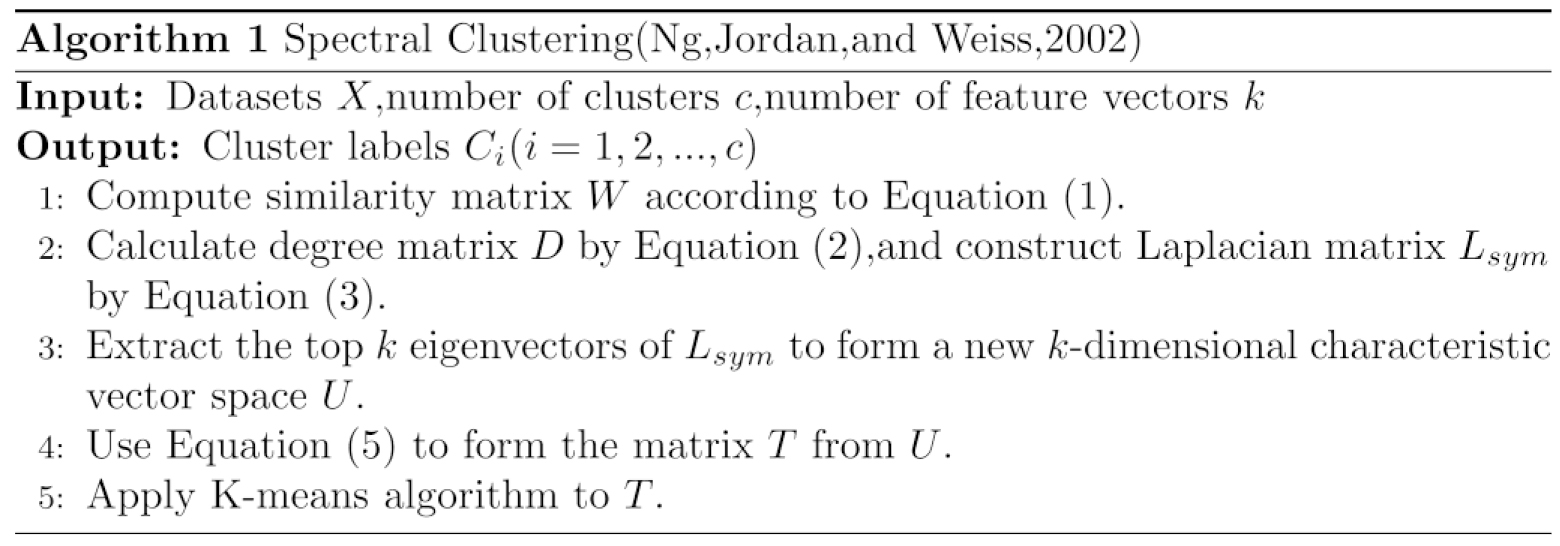
Finally, traditional clustering methods such as K-means algorithm are used for each row of $T$ . The cluster label for each row of $T$ is consistent with the cluster label for each row of data points in the original dataset $X$ .

Algorithm 1 shows the detailed steps of the spectral clustering algorithm proposed by Ng et al [9].

Compared with the traditional K-means algorithm, the SC algorithm has a significant improvement. On the one hand, the K-means algorithm only performs well on circular datasets or spherical datasets. The SC algorithm is applicable to datasets without considering their sample space of any shape. On the other hand, the K-means algorithm is easy to fall into the local optimal problem when the datasets are non-convex, but the SC algorithm can converge to the global optimal solution.

Although spectral clustering algorithms have been extensively studied, many problems still need to improve, including the following three aspects:

The construction of similarity matrix.

The earliest version of the SC algorithm directly uses the sample adjacency matrix to divide the graph [39]. The later SC algorithm uses the Gaussian kernel density function to construct the similarity matrix $W$ , but it only considers the Euclidean distance between the two sample points. In other words, it does not include the multivariate characteristics of the data. In addition, the value of $\sigma$ affects the quality of the similarity matrix $W$ , so this specific value takes many experiments to determine.

The selection of the figure for feature vectors.

In machine learning feature extraction, the maximum eigenvalue usually contains the maximum information in the direction of the feature vector [39]. The SC algorithm usually selects the feature vectors corresponding to the first $k$ eigenvalues. The essence of the above process is the statute of the dimension, which may lose a little information. This may lead to the problem that the optimized indicator vector does not fully indicate the attribution of each sample data.

The determination of the number of clusters.

The SC algorithm in low-dimensional solution space usually uses the K-means algorithm for two-stage clustering. Due to the randomness of the K-means algorithm in selecting cluster center points, it may cause empty clusters. It is also easy to fall into a local optimum. Besides, K-means algorithm needs to specify the number of clusters artificially. In a real-world scenario, it has no prior knowledge of the number of categories that are most appropriate for a given dataset. So, the determination of the number of clusters does affect the overall accuracy and stability of the SC algorithm.

4. Spectral clustering based on multi-scale threshold and density combined with shared nearest neighbors (MSTDSNN-SC) algorithm

By means of the analysis in Section 3, there is no doubt that the defects of the SC algorithm need to be optimized to meet the ever-changing application scenarios. A method on the basis of SC algorithm is proposed to solve all the above problems. In this part, we will elaborate on the improvements.

4.1 Optimization of similarity measures

Based on the characteristics of the spatial-temporal trajectory data collected by wireless network, it is far from enough to use the distance between the trajectories as a similarity measure. Most trajectory similarity measures are analyzed from the perspectives of time series of trajectories or spatial dimensions of trajectory points. The time series similarity focuses on the change of the series over time. The similarity based on the spatial dimension of trajectory points mainly considers the variation and distribution of trajectory points in geographic locations, and takes the spatial attributes as the main criterion for judging the similarity. The relationship between the information features of both temporal and spatial dimensions in spatial-temporal trajectories is independent of each other. Therefore, it is necessary to consider the time series and spatial information to quantify the similarity between the trajectories at the same time. We draw on the STD-STDSS model originally used to measure user similarity in the literature [40] and introduce the popularity of location visits to modify the time distance model.

In fact, the time and space characteristics are mutually constrained but independent of each other. In previous studies, the value of similarity results has been defined between 0 and 1. Similarly, we define a collection of trajectory sequences $\textit{Route}=\{R_{1},R_{2},\ldots R_{n}\}$ and choose any two spatial-temporal trajectory sequences from Route, noted as $R_{i}=\{r_{i,1},\ldots,r_{i,x},\ldots,r_{i,K_{i}}\}(1\leqslant x\leqslant K_{i})$ and $R_{j}=\left\{r_{j,1},\ldots,r_{j,y},\ldots,r_{j,K_{j}}\right\}(1\leqslant y% \leqslant K_{j})$ , where $K_{i}$ and $K_{j}$ are the total number of tracing points in the $R_{i}$ and $R_{j}$ respectively. $r_{i,x}$ and $r_{j,y}$ all represent trajectory points in the trajectory sequence. Taking $r_{i,x}$ as an example, it is actually a two-tuple $(l_{i,x},t_{i,x})$ . $l_{i,x}\in S$ represents the location where the log record occurred in the wireless network, and $t_{i,x}$ represents the time when the log record occurred. The set $S=\{s_{1},s_{2},\ldots,s_{M}\}$ represents $M$ disjoint locations. Then we define the time similarity $\textit{TCor}(R_{i},R_{j})$ and spatial similarity $\textit{SCor}(R_{i},R_{j})$ between $R_{i}$ and $R_{j}$ . According to the literature [40], similarity properties can be considered when there are shared properties between systems with different eigenvalues. The degree of similarity between things can be expressed by numerical quantitative analysis, taking values between 0 and 1. Therefore, the range of values of $\textit{TCor}(R_{i},R_{j})$ and $\textit{SCor}(R_{i},R_{j})$ is $\left[{0,1}\right]$ .

First, we follow the method of calculating spatial similarity in the literature [40], i.e., we begin with the basic judgment of spatial similarity based on the longest common subsequence (LCSS) [41] and obtain a set of common subsequences $R_{\textit{LCSS}}$ . LCSS is to find the longest subsequence of the common subsequence of two given sequences by matching only the same sequence points. This subsequence appears in the same order in both sequences, but is not required to be consecutive. Therefore, it can be assumed that the longer the length of LCSS, the more similar the given two sequences are. As a result, for trajectories $R_{i}$ and $R_{j}$ , their LCSS sequences can be written as $R_{\textit{LCSS}}=\{r_{\textit{LCSS,1}},r_{\textit{LCSS,2}},\ldots,r_{\textit{% LCSS,z}},\ldots,r_{\textit{LCSS},K_{\theta}}\}$ . $K_{\theta}$ is the length of the LCSS sequence $R_{\textit{LCSS}}$ . On this basis, we introduce the continuity factor $\gamma_{i\to j}$ [42] and modify the expression of spatial similarity between trajectories $R_{i}$ and $R_{j}$ to enhance the metric of spatial similarity. The spatial similarity $\textit{SCor}(R_{i},R_{j})$ can be given as follows:

$\displaystyle\gamma_{i,j}=\frac{(\gamma_{i\to j}+\gamma_{j\to i})}{2}$

(6) $\displaystyle\textit{SCor}(R_{i},R_{j})=\left(\left(\left.\frac{K_{\theta}}{K_% {i}}+\frac{K_{\theta}}{K_{j}}\right)\right/2\right)\times\gamma_{i,j}$

A larger $K_{\theta}$ means that $R_{\textit{LCSS}}$ is longer and $\textit{SCor}(R_{i},R_{j})$ is higher. If $R_{\textit{LCSS}}=\emptyset$ , it can be considered that there is no spatial similarity. Therefore, it can be further inferred that $\textit{SCor}(R_{i},R_{j})$ is also zero.

Then, the time distance between $r_{i,x}$ and $r_{j,y}$ can be written in terms of $\textit{Dis}(r_{i,x},r_{j,y})$ [43]. For those trajectory sequences that have spatial similarity after preliminary judgment, the temporal similarity is calculated based on the shortest time distance. However, as described in the literature [43], if too many people visit the location within a unit time, there is a higher chance of an actual unrelated trajectory at that location in the real world. Therefore, if the access frequency of a certain place is too high, the time distance increases as the correlation between any track records decreases. As a result, we introduce location popularity for calculating $\textit{Dis}(r_{i,x},r_{j,y})$ .

Let $s_{p}$ denote a place in the set $S$ and $W_{p}$ be the location popularity of $s_{p}$ [43]. The following equation should be used to modify the influence of different locations.

$\displaystyle W_{p}=\frac{\textit{visits}_{p}}{\sum\limits_{i=1}^{N}{\textit{% visits}_{i}}}$ (7)

where $N$ is the number of wireless network access points, $\textit{visits}_{p}$ is the number of accesses to the wireless network access point corresponding to the location $s_{p}$ .

After adding the location popularity, here is the formula for calculating the redefined time distance.

$\displaystyle\textit{WDis}(r_{i,x},r_{j,y})=\left\{{\begin{array}[]{l@{\ \ }l}% W_{p}\left|{t_{i,x}-t_{j,y}}\right|\ \ &l_{i,x}=l_{j,y}=s_{p}\\ \infty\ \ &l_{i,x}\neq l_{j,y}\\ \ \ \end{array}}\right.$ (8)

Taking the tracing point $r_{i,x}$ in the trajectory sequence $R_{i}$ as an example, the smallest time distance is defined as:

$\displaystyle\textit{WSTD}(r_{i,x},R_{j})=\mathop{\min}\limits_{y}\textit{WDis% }(r_{i,x},r_{j,y})$ (9)

If the locations of the recording points are not the same, it can be considered that there is no similarity between $r_{i,x}$ and $r_{j,y}$ . Otherwise, the time similarity is related to the time difference between the two recording points, i.e., the smaller the time distance, the higher the time similarity. As the time distance increases, the time similarity also tends to 0.

Therefore, the time similarity of trajectory $R_{i}$ with respect to trajectory $R_{j}$ can be obtained by the sum of the time similarities of all tracing points in $R_{i}$ and the corresponding WSTD matching trajectory points in $R_{j}$ , denoted as $\textit{Cor}(R_{i},R_{j})$ , as expressed by:

$\displaystyle\textit{Cor}(R_{i},R_{j})=\frac{1}{K_{i}}\sum\limits_{x=1}^{K_{i}% }{\frac{1}{1+\textit{WSTD}(r_{i,x},R_{j})^{2}}}$ (10)

From the calculation process, it can be found that the calculation results of the WSTD model have asymmetry. Thus, the time similarity between $R_{i}$ and $R_{j}$ can be taken from Eq. (11). Therefore, the time similarity between the two trajectories is symmetric.

$\displaystyle\textit{TCor}(R_{i},R_{j})=\frac{\textit{Cor}(R_{i},R_{j})+% \textit{Cor}(R_{j},R_{i})}{2}$ (11)

Eventually, the spatial-temporal similarity $\textit{TSCor}(R_{i},R_{j})$ between any two trajectories is displayed in Eq. (12).

$\displaystyle\textit{TSCor}(R_{i},R_{j})=\textit{TCor}(R_{i},R_{j})\times% \textit{SCor}(R_{i},R_{j})$ (12)

The preliminary result of the trajectory similarity measurement calculated through the above steps should be between 0 and 1. Moreover, if $\textit{TSCor}(R_{i},R_{j})$ is close to 1, it shows that the correlation between the trajectories is very strong. The above-mentioned similarity measurement method not only eliminates interference data, but also retains the sequential characteristics of the trajectory space information. This approach therefore greatly improves the accuracy of the metric and ensures the reliability of subsequent clustering results.

Based on the above process, the construction of each element in the initial similarity matrix $W\in R^{n\times n}$ can be summarized as the following Eq. (13):

$\displaystyle\left\{{\begin{array}[]{ll}w_{i,i}=0&i=j\\ w_{i,j}=\textit{TSCor}(R_{i},R_{j})&i\neq j\\ \end{array}}\right.$ (13)

According to the description in Section 3, the SC algorithm clusters the data uses the similarity matrix or the eigenvectors in the Laplacian matrix to divide the data during the clustering process. Therefore, each of the clusters can be regarded as connected components to a certain extent. The intersections between different clusters affect the construction of the similarity matrix, leading to the propagation of misinformation. The accuracy of the final clustering is affected [44]. For these considerations, taking the trajectory $R_{i}$ as an example, we form a set $W_{N}(R_{i})=[w_{i,1},\ldots w_{i,p}]$ of $p$ trajectories having higher correlation with it and further introduce the corresponding local covariance matrix $\textit{LC}_{i}\in R^{p\times p}$ . Following the results of several experiments, the value of $p$ does not affect the accuracy of the subsequent experimental results, so we set the value of $p$ to 10. The matrix $\textit{LC}_{i}$ is expressed by:

$\displaystyle\textit{LC}_{i}=\frac{1}{p-1}\sum\limits_{k=1}^{p}{(w_{i,k}-\mu)}% (w_{i,k}-\mu)^{T}(i=1,2,\ldots,n)$ (14)

where $\mu$ denotes the mathematical expectation. By calculating the local covariance matrix $\textit{LC}_{i}$ , the relationships within similar samples become closer. In this way, the intersection points achieve a certain degree of separation. However, when the angle between different clusters is small using covariance alone does not ensure a very stable separation of intersections. So after decomposing the matrix $\textit{LC}_{i}$ , the matrix $Q_{i}$ is formed by the eigenvectors corresponding to the eigenvalues [25]. On the basis of the spatial scale threshold $\varepsilon$ , calculate the threshold $\eta$ in accordance with the local covariance matrix [13]:

$\displaystyle\eta=\mathop{\text{median}}\limits_{(i,j):w_{i,j}\leqslant% \varepsilon}\left\|{Q_{i}-Q_{j}}\right\|$ (15) $\displaystyle\varepsilon=\mathop{\max}\limits_{i}\min\limits_{\begin{subarray}% {c}j\\ j\neq i\end{subarray}}(1\leqslant i\leqslant n)$

The spatial scale threshold is chosen to make sure that the set of neighbors of each data point has a sufficient number of samples, which may include some intersection points to ensure the connectivity between each small subset. At the same time, the value of $\varepsilon$ is small enough to satisfy the previous condition, so that the data points in the neighborhood are as close as possible to the central data point. The approximation strategy is used to obtain a relatively optimal spatial scale threshold to more accurately express the similarity between the data. Similarly, the covariance scale threshold must be chosen to ensure not merely that the local covariance ranges of the neighbor sets of each data point are the same, but also that the local covariances of the different neighbor sets near the intersection are separate. As a result, it is better able to assign pairs of data points with high similarity to the same category, and those with low similarity to different categories. In this way, the limitation of multiple scale thresholds is combined with the initial similarity matrix W to jointly determine the final similarity matrix W_final. The influence of special sample points on the clustering results is avoided while retaining the similarity measures in the initial similarity matrix. Each element in the W_final can be shown by the following formula:

$\displaystyle\textit{w\_final}_{i,j}=\left\{{\begin{array}[]{ll}1,&w_{i,j}% \leqslant\varepsilon\ \text{and}\ \left\|{Q_{i}-Q_{j}}\right\|\leqslant\eta\\ 0,&\text{otherwise}\\ \end{array}}\right.$ (16)

If $\textit{w\_final}_{i,j}$ is 1, it is considered that there is a strong similarity between the row and column trajectories corresponding to the element. If $\textit{w\_final}_{i,j}$ is 0, the similarity between the row and column trajectories corresponding to the element is weak or even no similarity.
4.2 Selection of the number of eigenvectors

Step 3 of Algorithm 1 mentioned in Section 3 is essentially statute of the dimension, i.e., reducing the dimensionality from $d$ to $k$ , which is consistent with the role of PCA. According to the literature [25], PCA not only reduces the high dimensional data, but also removes the noise and finds the data in the hidden patterns. The top $k$ principal components with a cumulative contribution greater than 95 % are selected to contain most of the information. In order to avoid manual selection of the number of eigenvectors and make the selected characteristic variables retain as much information of the original variables as possible, we use the PCA algorithm to select the top $k$ principal components. Specifically, we start by centralizing the similarity matrix W_final. Then we calculate the covariance matrix and take out the top $k$ eigenvectors with a cumulative contribution of 95% to form the matrix $\Psi$ , where $\Psi$ can be formulated as follows.

$\displaystyle\Psi=\left[{{\begin{array}[]{c}{\psi_{1}^{T}}\\ {\psi_{2}^{T}}\\ \vdots\\ {\psi_{k}^{T}}\\ \end{array}}}\right]_{k\times n}$ (17)

With this method, the number of eigenvectors does not need to be manually specified. Then the selected $k$ principal components are directly used to construct the subsequent characteristic vector space $U\in R^{n\times k}$ .The matrix U can be ascribed in the following form.

$\displaystyle U^{T}=\Psi\textit{W\_final}$ (18)

Finally, the matrix $U$ is normalized to obtain the matrix $T\in R^{n\times k}$ .

4.3 Determination of the number of clusters

Generally, after dimensionality reduction, it is also necessary to use the traditional K-means clustering algorithm to cluster each row vector of the matrix $T$ . Using K-means clustering algorithm causes different clusters due to different initial cluster center. Besides, it also needs to manually specify the number of clusters. Taking into account the above shortcomings, we introduce the consideration of tracking points density [45].

There have been many algorithms in the research of density clustering. DBSCAN algorithm is a typical density clustering algorithm. Compared with K-Means, it is suitable for both convex and non-convex data sets. The DBSCAN algorithm clusters based on the idea of ??high-density connected regions, that is, the regions in the space that are sufficiently dense and meet the connectivity conditions are marked as the same cluster. It requires the input of two parameters $r$ (neighborhood radius) and $\varphi$ (the threshold of the core point). Based on this, the density is defined as the number of objects in a circular area with an object as the center and r as the radius in the space. For a certain object $t_{j}\in T$ , its $r$ -neighborhood contains the sub-sample set whose distance from $t_{j}$ is not greater than $r$ in the sample set $T$ , which can be expressed as $N(t_{j})=\{t_{i}\in T\left|{\textit{distance}(t_{i},t_{j})}\right.\leqslant r\}$ . The specific process of the DBSCAN algorithm is that if its density is greater than $\varphi$ , it is identified as the core point. A cluster with $t_{j}$ as the core object is created. Then the algorithm iteratively clusters all objects that meet the direct density reachability of the core object into one category. When no new points are added to any cluster, the iteration process ends. The DBSCAN algorithm can find clusters of any shape and does a good job of finding noise. However, the two parameters required by the algorithm are global parameters, which are not easy to control and determine. Subtle differences in parameter selection can cause huge differences in experimental results.

Although the parameters required by the DBSCAN algorithm are often determined by the k-distance graph, the position of the inflection point in the image may be difficult to determine in actual applications. So, we consider improving the selection of the parameters of the algorithm. In response to this problem, many different density definitions and corresponding clustering algorithms have appeared in recent years [46]. We noticed that in contrast to the DBSCAN algorithm, which defines the density as the number of data points in a given neighborhood, the k-nearest neighbor model can dynamically represent the local distribution characteristics. What’s more, only one parameter needs to be set and it is easy to select. However, when the k-nearest neighbor model is used to deal with high-dimensional data sets, it also becomes inaccurate in measuring local density due to the sparsity of the high-dimensional data space. Then a special similarity measure based on the K-nearest neighbor algorithm was proposed, named The Shared Nearest Neighbor (SNN) [47]. It is different from the traditional similarity measure. SNN is based on a kind of intermediate information to express similarity, i.e., the similarity of objects is measured by the “neighbors” shared between them. The specific realization of SNN is to find common neighbors from the set of k-nearest neighbors of two objects. The more common neighbors, the higher the similarity of the two objects, and vice versa. This method not only maintains the advantages of the k-nearest neighbor model, but is also suitable for high-dimensional spaces. We are inspired by the literature [48] and decide to combine the DBSCAN algorithm with shared neighbor affinity to solve the above shortcomings. The specific implementation process is as follows.

Considering each row of the matrix T obtained in Section 4.2 as a data point, it can be written as $T=[t_{1},t_{2},\ldots,t_{j},\ldots t_{n}]^{T}$ . For any data point $t_{j}\in T$ that has not been marked, define the $\tau$ neighborhood space of $t_{j}$ as $N_{\tau}(t_{j})=\{t_{1},\ldots,t_{\tau}\left|{t_{i}\in T,\forall z\in T-\{t_{1% },\ldots,t_{\tau}\},}\right.\textit{distance}(t_{j},t_{i})\leqslant\textit{% distanc}(t_{j},z)\}$ . And the KNN distance of $t_{j}$ is described as the average value of the distance between $t_{j}$ and $\tau$ neighbors, denoted as $\text{distance}\textit{KNN}(t_{j})$ , the specific formula is shown as Eq. (19).

$\displaystyle\text{distance}\textit{KNN}(t_{j})=\frac{1}{\tau}\sum\limits_{t_{% i}\in N_{\tau}(t_{j})}{\textit{dis}\text{tance}(t_{j},t_{i})}$ (19)

The KNN distance reflects the local distribution of the data point. The smaller the KNN distance, the denser the neighbors around the data point. Then the data point is more likely to be distributed in the dense area. Otherwise, the more likely it is to be distributed in the sparse area.

As for the number of SNN of $t_{j}$ , it refers to the number of shared neighbors of $t_{j}$ and its $\tau$ neighbors, denoted as $\textit{SNN}(t_{j})$ :

$\displaystyle\textit{SNN}(t_{j})=\sum\limits_{t_{i}\in N_{\tau}(t_{j})}{\left|% {N_{\tau}(t_{j})\cap N_{\tau}(t_{i})}\right|}$ (20)

where $\left|{N_{\tau}(t_{j})\cap N_{\tau}(t_{i})}\right|$ represents the number of elements shared by the $\tau$ -neighbor space of $t_{j}$ and $t_{i}$ .We think it is reasonable that the larger the sum of neighbors shared by the two data points, the higher the similarity of the two data points. Therefore, we update the concept of r-neighborhood here, i.e., the set of data points that share close neighbors with data point $t_{j}$ in the sample set $T$ . The concept is reflected by Eq. (4.3).

$\displaystyle N(t_{j})=\{t_{i}\in T\left|{\textit{SNN}(t_{i},t_{j})}\right.>0\}$ (21) $\displaystyle\textit{SNN}(t_{i},t_{j})=\left|{N_{\tau}(t_{j})\cap N_{\tau}(t_{% i})}\right|$

Based on Eqs (20) and (4.3), the concept of shared neighbor affinity is now given, that is, the ratio between the number of shared neighbors of the object and the KNN distance. We denote the shared neighbor affinity as $\textit{AffinitySNN}(t_{j})$ , which is represented as follows.

$\displaystyle\textit{AffinitySNN}(t_{j})=\frac{\textit{SNN}(t_{j})}{\textit{% dis}\text{tanc}\textit{eKNN}(t_{j})}$ (22)

It can be found from Eq. (22) that the greater the number of shared neighbors of an object and the smaller the KNN distance, the greater its SNN affinity. This indicates that the greater the degree of affinity between an object and $\tau$ neighbors, the greater the local density of the object. Then the determination of the core point is no longer based on the number of data points in a given neighborhood range greater than $\varphi$ , but the SNN affinity of the core point is greater than the average value of the SNN affinity of its $\tau$ neighbors. We summarize the conditions that the core points need to meet as follows:

$\displaystyle\textit{AffinitySNN}(t_{j})\geqslant\frac{1}{\tau}\sum\limits_{t_% {i}\in N_{\tau}(t_{j})}{\textit{AffinitySNN}(t_{i})}$ (23)

The above formula shows that the affinity of the core points is higher than the average level of their neighbors, so the core points are distributed in dense areas in space and have a greater similarity with their neighbors.

To sum up, we restate a DBSCAN algorithm process based on shared nearest neighbors as shown in Algorithm 2.

4.4 MSTDSNN-SC algorithm process

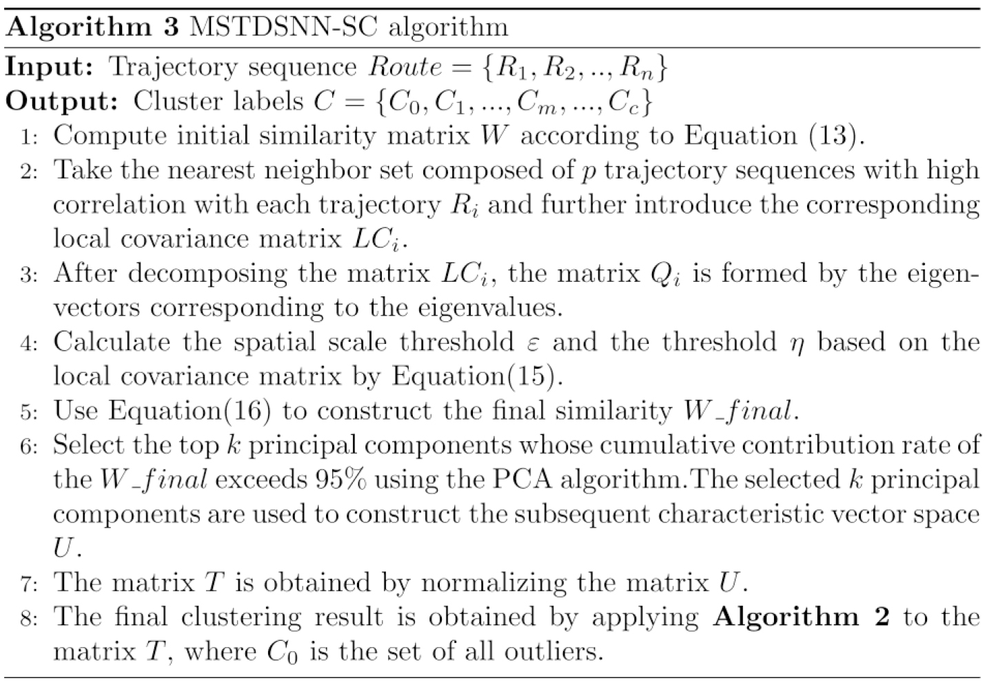
The whole process of the MSTDSNN-SC algorithm still includes three major steps: the establishment of similarity matrix, the construction of feature vector space, and low-dimensional subspace quadratic clustering.

Suppose a trajectory sequence dataset $\textit{Route}=\{R_{1},R_{2},\ldots R_{n}\}$ and the number of neighbors $p$ is given. Clustering aims to divide the dataset Route into $c$ classes. $c$ is the number of clusters. The set of cluster labels is $C=\{C_{0},C_{1},\ldots C_{c}\}$ . It should be noted that the cluster $C_{0}$ is actually a temporary collection of all outlier points. When the clustering results are subsequently evaluated, each outlier is treated as a separate class. The process of the MSTDSNN-SC algorithm is shown in Algorithm 3 below.

5. Experiments

In order to verify the accuracy and effectiveness of the MSTDSNN-SC algorithm for detecting abnormal trajectories, we use a real campus network data set of from a certain area of China as an example, and compares it with several clustering algorithms, including the K-means algorithm, Spectral clustering algorithm, DBSCAN algorithm, Affinity Propagation (AP) clustering algorithm, Spectral Clustering Algorithm Based on Message Passing (MPSC) algorithm, DBSCAN algorithm based on the similarity matrix between the geodesic distance and share nearest neighbors (GS-DBSCAN) algorithm and spectral clustering algorithm based on local covariance matrix (LCSC) algorithm, etc. The MPSC algorithm is a combination of AP clustering and spectral clustering, while the GS-DBSCAN algorithm constructs a similarity matrix based on geodesic distances and shared nearest neighbors and then performs clustering using the DBSCAN algorithm. The LCSC algorithm uses the local covariance matrix to set a threshold to construct a similarity matrix and then uses the spectral clustering algorithm.

5.1 Experimental data set and metrics

In fact, the real university spatial-temporal trajectory data comes from the log records of 6202 student users who stayed at nearby access points after accessing the campus wireless network, which spans four months. Each of these folders stores the Internet log files of all student users for each day. Table 1 shows the format of the original spatial-temporal trajectory data. Each row represents a trajectory sampling point, including phone MAC address, access point MAC address, received signal strength indicator(RSSI), time and other information data.

Table 1
Original data format

Phone MAC address	Access point MAC address	Received signal strength indicator (RSSI)	Time
5c:c3:::09:**	00:34::a4::fe	$-$ 54	2019-10-01 00:00:00
74:c1:::f0:**	00:34::94::c0	$-$ 76	2019-10-01 16:34:58
3c:a6:::98:**	00:34::a4::1a	$-$ 72	2019-10-01 23:59:59

As we know, the evaluation metrics of the clustering algorithm usually include internal and external indicators. Internal indicators are suitable for the situation of unknown data labels, while external indicators have a good reflection on the data with known data labels. As the datasets used in this experiment do not have labels, several internal evaluation metrics are used to judge the accuracy of clustering results, with the inclusion of Silhouette Coefficient (SI) [49], Davies-Bouldin Index (DB) [50], Calinski-Harabasz Index (CH) [51] and Dunn Index (DVI) [52]. The meaning and calculation methods of these indicators are illustrated below.

SI measures how similar each point is in its own cluster compared to the points in other nearest clusters. The expression of SI is explained as Eq. (24).

$\displaystyle\textit{SI}=\frac{1}{c}\sum\limits_{i=1}^{c}{\frac{1}{n_{i}}}\sum% \limits_{t_{i}\in C_{i}}{\frac{(b(t_{i})-a(t_{i}))}{(\max([b(t_{i}),a(t_{i})])% )}}$ (24)

where $a(t_{i})$ represents the average inconsistency between $t_{i}$ and all other points in the same class similarity, $b(t_{i})$ represents the minimum average dissimilarity between $t_{i}$ and points in other classes. $c$ is the number of categories and $n_{i}$ is the number of data points in the cluster $C_{i}$ . The SI value range of each point is between $-$ 1 and 1. The closer the index is to 1, the more suitable the point is to be classified into the current cluster. The closer the index is to 0, the more likely the point may be located at the edge of the cluster.

After calculating SI for each point, the average value is computed to obtain the SI of the clustering results. A higher SI value means a better class division.

DB is the maximum value of the ratio of the sum of the average distances between any two categories of within-class distances to the centroid distance between the two clusters. It can be calculated by Eq. (25):

$\displaystyle\textit{DB}=\frac{1}{c}\sum\limits_{i=1}^{c}{\mathop{\max}\limits% _{j\neq i}}\left({\frac{\sigma_{i}+\sigma_{j}}{\text{distance}\left({C_{i},C_{% j}}\right)}}\right)$ (25)

where $\sigma_{i}$ is the sum of the average distances from all points in the cluster $C_{i}$ to the centroid of the cluster $i$ . $\sigma_{j}$ has a similar meaning. $\text{distance}\left({C_{i},C_{j}}\right)$ is the distance between the centroids of $C_{i}$ and $C_{j}$ . The smaller DB value means that the clustering result is close to the inside of the cluster, and different clusters are separated farther. In other words, this shows that the smaller the between-class distance, the larger the within-class distance.

CH measures the compactness within the class by calculating the sum of squares of the distances between each point in the class and the center of the class, and measures the separation of the dataset by calculating the sum of the squares of the distances between various centers and the center of the dataset. CH is obtained from the ratio of separation and compactness. The definition of CH is shown in Eq. (26).

$\displaystyle\textit{CH}=\frac{\textit{Tr}\left({S_{B}}\right)/C_{i}-1}{% \textit{Tr}\left({S_{W}}\right)/c-C_{i}}$ (26)

where $\textit{Tr}\left({S_{B}}\right)$ represents the trace of the inter-class deviation matrix, and $\textit{Tr}\left({S_{W}}\right)$ represents the trace of the within-class deviation matrix. $C_{i}$ refers generically to each cluster obtained from the clustering division. The larger CH indicates that the cluster itself is closer and the clusters are more scattered, i.e., the better clustering results.

The definition of DVI is the ratio of the shortest distance between any two clusters to the maximum distance within any cluster.

$\displaystyle\textit{DVI}=\frac{\mathop{\min}\limits_{0<i\neq j<c}\left\{\min% \limits_{\begin{subarray}{c}\forall t_{i}\in C_{i}\\ \forall t_{j}\in C_{j}\end{subarray}}\text{distance}\left(t_{i},t_{j}\right)% \right\}}{\mathop{\max}\limits_{0<i<c}\mathop{\max}\limits_{0<j<c}\left\{{% \text{distance}\left({t_{i},t_{j}}\right)}\right\}}$ (27)

The larger the DVI value, the closer the clustering results are within the same cluster, and the farther the separation between different clusters.

5.2 Data preprocessing

Due to many factors such as signal strength of base station, user type, storage method, etc., the collected spatial-temporal trajectory data cannot be directly applied to subsequent data mining work. Hence, the spatial-temporal trajectory data must be preprocessed first. In detail, we collect the list of all enrolled students and extract the valid information including student name, apartment number, gender, mobile MAC address, college, class, and major. The first step is to match the cell phone MAC address of each trace sampling point in the original data set with the device MAC address of Stu A. If the match is successful, it means that the trace sampling point is Stu A’s trace, then the trace data point will be temporarily saved. Thus, we create a separate trace log file for each student user, and set the name as Class-Name-Number-Trace. Here, we take Class1-Stu A-No.0001-Trace file as an example to show the detailed process of data pre-processing. The first step is to match the cell phone MAC address of each trace sampling point in the original data set with the device MAC address of Stu A. If there is a successful match, it means that the trace sampling point is Stu A’s trajectory. So, we temporarily save the trajectory data point. Then, we do the following processing on these temporarily saved trajectory sampling points.

5.2.1 Format conversion

The original spatial-temporal trajectory data is recorded in computer language format, involving UNIX time format and base station code. Therefore, it is necessary to transform the data into a special format before it can be used in the subsequent data mining work. We represent the time data of each trajectory point in the data set as the whole number of days and their fractional values since January 0, 0000, so that the 24-hour time of a day is converted to between $[0,1]$ .

5.2.2 Data cleaning

Students will produce duplicate redundant information in the process of surfing the Internet, and we compress and merge the trajectory points with the same location area and time interval within 5 minutes according to the actual demand. And the intermediate value of the time data is taken as the new time data after merging. In addition, the noise data caused by abnormal acquisition equipment and other reasons can also have an impact on the subsequent method. Here we combine the RSSI and reject it by judging whether the time stamp of the latter track point is larger than that of the previous track point.

5.2.3 Anonymous processing

In order to protect the user’s private information, the key private information in the original spatial-temporal trajectory data must be anonymized to make it impossible to trace the source.

5.2.4 Map matching

Suppose Stu A creates a series of behavior records in the wireless network as $R:\{(\text{AP6},t_{1}),(\text{AP6},t_{2})$ , $(\text{AP7},t_{3}),(\text{AP8},t_{4}),(\text{AP3},t_{5}),(\text{AP3},t_{6}),(% \text{AP4},t_{7}),(\text{AP5},t_{8})\}$ . APx is the number of the network access point and $t_{1},t_{2},\ldots,t_{8}$ is the time when the connection behavior occurs. As a general rule, the access points in wireless networks are deployed and distributed in various buildings, so the mapping relationship between access points and buildings in real maps can be established to simplify the trajectory sequence. Moreover, the category and functional information of buildings can bring more hidden semantic information to the trajectory sequence for better understanding and application of mining results. Therefore, we can represent the spatial-temporal trajectory sequence according to the actual mapping relationship as $R:\{(\text{B4},t_{1}),(\text{B4},t_{2}),(\text{B4},t_{3}),(\text{B4},t_{4}),(% \text{B2},t_{5}),(\text{B2},t_{6}),(\text{B2},t_{7}),(\text{B3},t_{8})\}$ . It is easy to see that AP6 and AP5 are located in buildings B4 and B5 respectively. AP7, AP8, AP3 and AP4 are located in building B2. In this way, the original spatial-temporal trajectory sequence consisting of a series of login access points and connection occurrence times is converted into a sequence set formed by a binary group of location numbers and connection occurrence times.

The trajectory information data obtained after the above processing is stored in the trajectory log file of Stu A. In the log file, trajectories are points ordered by time. Each point contains normalized x and y coordinates, Internet access location, time and other information. Given that the spatial-temporal trajectory data recorded in the wireless network covers a long period of time, in order to reduce the subsequent computation time, a parallel sliding time window method is also needed for adaptive segmentation before the similarity metric is performed.

After obtaining the preprocessed trajectory data, we randomly select 50 users with complete Internet records, and extract their trajectories within four months to form their individual spatial-temporal trajectory dataset, referred to as the ISST dataset. In addition, we select any 5000 trajectories from all users to form the group spatial-temporal trajectory dataset, which is referred to as the GSST dataset. These two datasets are used in our experiments in subsequent chapters.

5.3 Parameter selection

In this paper, several different clustering algorithms and MSTDSNN-SC algorithm are used for comparative experiments. Among them, K-means algorithm, DBSCAN algorithm and AP clustering algorithm all use the results of similarity matrix W_final for subsequent clustering. MPSC, GS-DBSCAN and LCSC use the similarity matrix calculated by the similarity function proposed in their respective papers. In addition, in order to better verify the necessity and rationality of the improved MSTDSNN-SC algorithm, we set up the following comparative experiments, which are: the traditional SC algorithm by using the initial similarity matrix $W$ is referred to as Original-SC algorithm; the traditional SC algorithm by using the similarity matrix W_final is referred to as MSTK-SC algorithm; the SC algorithm by using the initial similarity matrix $W$ and using the Algorithm 2 for final clustering is referred to as the DB-SC algorithm; the SC algorithm by using the similarity matrix W_final and using the DBSCAN algorithm for final clustering is referred to as the MSTD-SC algorithm.

The parameters that need to be determined in the MSTDSNN-SC algorithm is the number of nearest neighbors $\tau$ used to calculate SNN. In order to analyze the impact of $\tau$ on the algorithm, User_3 in the ISST dataset is used as shown in Fig. 1.

To select the optimal nearest neighbors, we increase the number of neighbors $\tau$ from 3 to 120. For the determination of the lower limit, if the number of neighbors of a data point is small and the density is sparse, it means that there is no similarity between the two data points. In addition, the error may be caused by too small $\tau$ . Therefore, we set the lower limit to 3. If the upper limit of $\tau$ is too large, it increases the complexity of the algorithm. Analysis shows that too high $\tau$ has no effect on the results of the algorithm, so it has little meaning for further testing.

It can be seen from Fig. 1 that when $\tau$ is between 5 and 50, the CH and DB indicators fluctuate significantly. After that, the change trends of the selected indicators for SI, DB, CH, and DVI are roughly the same. Thus, we can replace multiple indicator changes with one indicator change. Furthermore, it is obvious that as $\tau$ increases, the value of each indicator tends to stabilize. However, an exorbitant $\tau$ value leads to the decrease of indicators. The value of $\tau$ should be determined in advance through experiments, otherwise the optimal clustering results cannot be obtained. In the case of the ISST dataset, when $\tau=$ 65, each indicator value is higher, so 65 could be selected as the best neighbor number of the ISST dataset. Similarly, in the GSST dataset, the four index values are all optimal with $\tau=$ 1200.

The specific parameter settings of the above algorithm used in ISST dataset are summarized in Table 2. Table 3 shows the specific parameter settings of the above algorithm used in GSST datasets.

Table 2
Comparison experiment parameter in ISST dataset

Algorithm	Parameters and values
K-means	$c$ is determined according to each dataset
Original-SC algorithm	$c$ is determined according to each dataset, $k=$ 6
MSTK-SC algorithm	$c$ is determined according to each dataset, $k=$ 6
DB-SC algorithm	$k=$ 6, $r=$ 309.4, $\varphi=$ 6
DBSCAN algorithm	$r=$ 40, $\varphi=$ 5
AP clustering algorithm	damping factor $=$ 0.7, preference $=$ median (median (W_final))
MPSC algorithm	$k=$ 6, damping factor $=$ 0.7, preference $=$ median (median (W_final))
GS-DBSCAN algorithm	$l=$ 7, $r=$ 10 ${}^{-8}$ , $\varphi=$ 4
LCSC algorithm	$c$ is determined according to each dataset, $k=$ 6
MSTD-SC algorithm	$r$ and $\varphi$ are determined by k-distance graphs, $p=$ 10
MSTDSNN-SC algorithm	$\tau=$ 65

Table 3

Comparison experiment parameter settings in GSST dataset

Algorithm	Parameters and values
K-means	$c=$ 21
Original-SC algorithm	$c=$ 20, $k=$ 6
MSTK-SC algorithm	$c=$ 20, $k=$ 6
DB-SC algorithm	$k=$ 6, $r=$ 1455.1855, $\varphi=$ 22
DBSCAN algorithm	$r=$ 29.2233, $\varphi=$ 18
AP clustering algorithm	damping factor $=$ 0.7, preference $=$ median (median (W_final))
MPSC algorithm	$k=$ 6, damping factor $=$ 0.7, preference $=$ median (median (W_final))
GS-DBSCAN algorithm	$l=$ 7, $r=$ 10 ${}^{-8}$ , $\varphi=$ length(data)/25
LCSC algorithm	$c=$ 20, $k=$ 6
MSTD-SC algorithm	$p=$ 10, $r=$ 50.18, $\varphi=$ 14
MSTDSNN-SC algorithm	$\tau=$ 1200

Figure 1.

Changes in the various metrics of the ISST dataset.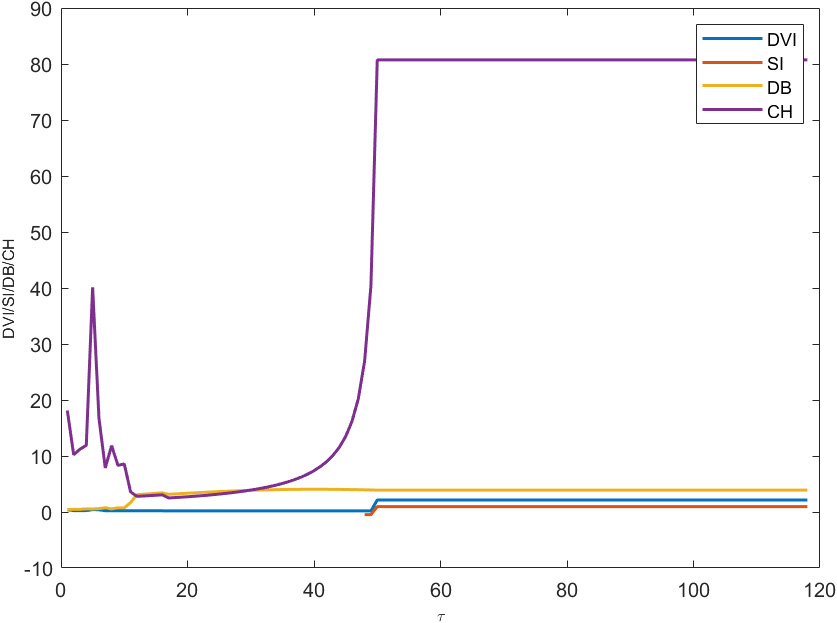

5.4 Experimental results and analysis

The simulation environment is MATLAB R2019a and executed on a 1.60 GHz Intel Core i5-8265U CPU equipped with 8 GB RAM and Windows 10.

5.4.1 Results of ISST dataset

The ISST data in this experiment is derived from the real campus wireless network Internet dataset after preprocessing. The related introduction is described in Sections 5.1 and 5.2. In the experiment, we select all the trajectory datasets of the same user in four months (September 2019 to December 2019). After the data preprocessing operation as described in Section 5.2, anomaly detection is performed separately for each user in the ISST dataset using the MSTDSNN-SC algorithm. We take the trajectory datasets of several users with relatively comprehensive data records as an example, and use the various clustering algorithms mentioned above to evaluate them separately. Table 4 shows the results in terms of SI, DB, CH and DVI on ISST dataset, where the symbol “/” indicates the meaningless parameters.

Table 4
Performances of clustering algorithms for ISST dataset

Algorithm	SI	DB	CH	DVI	NC	NO
User_1
K-means	0.6848	1.2394	112.4713	0.6787	5	/
DBSCAN algorithm	/	1.8916	56.8336	1.5571	51	5
AP clustering algorithm	/	0.7195	1.9128	0.3094	6	/
Original-SC algorithm	0.0860	3.4009	7.1886	0.2121	9	/
SC algorithm based on Kmeans using W_final (MSTK-SC algorithm)	0.8274	1.1916	828.6288	0.9728	6	/
SC algorithm based on DBSCAN using $W$ (DB-SC algorithm)	0.6116	3.7264	8.5010	2.3401	9	8
SC algorithm based on DBSCAN using W_final (MSTD-SC algorithm)	0.9407	3.4247	542.1938	8.7697	8	7
MPSC algorithm	0.8827	1.1768	38.2905	0.4428	2	/
GS-DBSCAN algorithm	/	0.7154	1.6974	0.5021	8	74
LCSC algorithm	0.7732	1.9148	196.5874	0.4528	5	/
MSTDSNN-SC algorithm	0.9575	1.8232	879.2246	8.7697	4	3
User_2
K-means	0.6884	1.2229	120.8870	0.9386	7	/
DBSCAN algorithm	/	1.9736	36.0810	1.3140	48	47
AP clustering algorithm	/	0.7251	2.0108	0.3192	59	/
Original-SC algorithm	0.3660	2.2838	874.9069	0.3877	9	/
SC algorithm based on Kmeans using W_final (MSTK-SC algorithm)	0.7883	1.0954	348.9304	0.7426	3	/
SC algorithm based on DBSCAN using $W$ (DB-SC algorithm)	0.6646	6.0274	1540.8368	0.9746	7	6
SC algorithm based on DBSCAN using W_final (MSTD-SC algorithm)	0.8288	3.4240	249.0614	1.1882	9	8
MPSC algorithm	/	/	/	/	1	/
GS-DBSCAN algorithm	/	0.7467	4.3772	0.6978	8	74
LCSC algorithm	0.8076	2.3349	205.8730	0.6479	7	/
MSTDSNN-SC algorithm	0.9463	1.9707	411.8096	1.3585	9	8
User_3
K-means	0.6493	0.9098	84.5313	1.1171	10	/
DBSCAN algorithm	0.7140	1.0274	72.7540	0.9487	15	1
AP clustering algorithm	0.4344	1.3108	3.5481	0.8344	3	/
Original-SC algorithm	$-$ 0.6970	2.7853	3.6942	0.0595	3	/
SC algorithm based on Kmeans using W_final (MSTK-SC algorithm)	0.4778	0.7971	57.3673	0.1949	3	/
SC algorithm based on DBSCAN using $W$ (DB-SC algorithm)	0.3764	7.1994	65.8194	0.7467	24	23
SC algorithm based on DBSCAN using W_final (MSTD-SC algorithm)	0.8383	4.10708	53.5604	1.3849	3	2
MPSC algorithm	/	/	/	/	1	/
GS-DBSCAN algorithm	/	0.5898	$-$ 7.2182	0.8515	86	8
LCSC algorithm	0.8225	0.9006	61.0420	0.3835	4	/
MSTDSNN-SC algorithm	0.9701	3.9092	80.7272	2.1420	4	3

As reported in Table 4, for the above three users, the SI of the MSTDSNN-SC algorithm is better than other clustering algorithms. Not only that, the SI of the MSTDSNN-SC algorithm is close to 1. According to the description in Section 5.1, it indicates that our algorithm can perform better in the clustering. What’s more, this conclusion can also be proved from the DVI indicator. As it is known for the introduction of Section 4.3, several related algorithms based on the DBSCAN algorithm can directly identify outliers, so the NO column shows the number of outliers that are temporarily classified as a cluster $C_{0}$ . Furthermore, the NC column shows the number of clusters. The NC of related clustering algorithms based on the K-means algorithm are given in advance. Besides, the NC of related clustering algorithms based on DBSCAN algorithm need to be determined indirectly by reading the parameters from the k-distance graph each time. However, a fixed $\tau$ value is selected by the improved method. Its variation over a wide range does not cause fluctuations in the clustering evaluation index. Although some algorithms achieve better performance than our algorithm on the indicators DB and CH, considering the number of clusters and the performance of other indicators, our algorithm still ranks in the top three on DB and CH.

For User_1, our algorithm achieves the best performance in the index evaluation of SI, CH and DVI, and the performance of CH and DVI is far higher than other algorithms. In the DB index, although the best DB value is obtained by using the GS-DBSCAN clustering algorithm, which is 0.7154. It can be known that the clustering result of the algorithm is not reasonable enough according to the value of NC and NO. The DB value of the AP algorithm ranks second in the order from small to large. The same reason is applicable to the AP clustering algorithm. In contrast, the MSTK-SC algorithm performs better than our algorithm in the evaluation of DB, but the results of the other three indicators are slightly inferior to MSTDSNN-SC algorithm. Moreover, the K-means algorithm is used in the MSTK-SC algorithm, so the result is not stable.

For User_2, there is also such a problem that the AP clustering algorithm is used to obtain the best DB value. It can still be inferred from the value of NC and NO that the clustering result of the algorithm is not reasonable enough. Additionally, the MSTK-SC algorithm, GS-DBSCAN algorithm and K-means algorithm achieve better DB values, but the results of the other three indicators are not as good as our algorithm. Furthermore, the parameter adjustment process in the above algorithms is also more troublesome.

For User_3, several algorithms that are better than our algorithm on the DB indicator also have the problem that their performance of the other three indicators is not as good as our algorithm. Especially for the Original-SC algorithm, SI even appears negative. Such a clustering result is obviously unjustifiable. In inclusion, the data in the NC and NO columns show that the class clusters divided by the GS-DBSCAN algorithm are not reasonable.

In reality, when evaluating the overall ISST dataset using the SI metric, our algorithm achieves a mean value of 0.9528 among 50 users. As described in Section 5.1, the closer the value of the SI metric is to 1, the better the clusters are. In other words, the clusters partitioned using the MSTDSNN-SC algorithm are reasonable. Through the analysis of the table, considering the clustering index evaluation results and the rationality of the number of clusters, our algorithm performs best and is the most stable. This is due to the fact that the construction of the similarity matrix not only fully considers information on the temporal and spatial dimensions of the trajectory and location popularity, but also processes the intersection points through multi-scale thresholds. And in the last step, the DBSCAN algorithm based on shared nearest neighbors is used to directly identify the abnormal trajectories while clustering. To sum up, the result is extremely reliable.

5.4.2 Results on GSST dataset

In this part, MSTDSNN-SC algorithm is subjected to further test with GSST dataset. Again, the performances of several algorithms are benchmarked in terms of SI, DB, CH and DVI. Table 5 displays the performance of clustering algorithms. The symbol “/” in the table means that the entries had no actual values.

Table 5
Performances of clustering algorithms on GSST dataset

Algorithm	SI	DB	CH	DVI	NC	NO
K-means	0.1616	2.1931	405.4131	0.8862	21	/
DBSCAN algorithm	$-$ 0.3826	1.0193	1.0075	0.6663	44	43
AP clustering algorithm	0.0317	3.4008	228.9421	0.6663	30	/
Original-SC algorithm	$-$ 0.9743	3.2035	0.0448	0.0016	20	/
SC algorithm based on K-means using W_final (MSTK-SC algorithm)	0.3660	1.5029	41564	0.0805	20	/
SC algorithm based on DBSCAN using $W$ (DB-SC algorithm)	0.9707	2.8936	47524	0.9168	28	27
SC algorithm based on DBSCAN using W_final (MSTD- SC algorithm)	0.9884	5.2133	35086	20.8711	16	13
MPSC algorithm	/	/	/	/	1	/
GS-DBSCAN algorithm	0.9959	0.7639	63.1360	50.1800	4979	4977
LCSC algorithm	0.3758	1.0339	1220.7050	1.1151	20	/
MSTDSNN-SC algorithm	0.9813	2.9566	37843	22.9604	14	12

As can be seen from Table 5, although the MSTDSNN-SC algorithm does not perform as well as K-means and DBSCAN algorithm in the evaluation of DB metrics, it performs best in all the other three metrics compared to the four classical algorithms. In particular, the DBSCAN algorithm achieved the best results in DB metrics, but its SI metrics showed negative values, which is obviously undesirable.

In a comparison between the Original SC algorithm and the DB-SC algorithm, it is not difficult to find that the metrics of all four categories are improved after replacing the K-means algorithm with the DBSCAN algorithm. Observing the metrics of MSTK-SC and Original SC algorithm separately, we can see that all four metrics improve after using the similarity matrix W_final. And our algorithm not only greatly outperforms the Original SC algorithm in the evaluation of the four categories of metrics, but also has fewer parameters compared to the MSTD-SC algorithm. Moreover, it is more stable than the clustering results obtained using MSTK-SC algorithm.

Before comparing with several clustering algorithms proposed in the last three years, the first thing to note is that the GS-DBSCAN algorithm has good evaluation results on the four indicators. But combined with the number of outliers as high as 4979 categories, it can be seen that the actual division effect of the algorithm is not convincing. Therefore, the performance of the GS-DBSCAN algorithm is not being analyzed below. Like the ISST dataset, the MSTDSNN-SC algorithm achieves very good evaluation results in the SI and DVI indicator, indicating evidence of great potential in clustering. Furthermore, our algorithm ranks second in the CH indicator evaluation. Although the MSTDSNN-SC algorithm does not look very good at first glance in the indicator DB, the LCSC algorithm performs poorly in the other three indicators. It should be noted that the MPSC algorithm did not achieve good results on our dataset, which is more suitable for low-dimensional datasets, depending on the analysis of the literature [11].

5.4.3 Analysis of anomaly detection results

The above-mentioned clustering evaluation indicators can only reflect the credibility of the results of the clustering algorithm. Whether the MSTDSNN-SC algorithm can effectively screen out possible abnormal trajectories still needs further verification. For this purpose, we treat each data point in cluster $C_{0}$ obtained by the MSTDSNN-SC algorithm as an outlier, and then we verify the filtered abnormal spatial-temporal trajectory data from two perspectives: the abnormal trajectory of the individual user and the abnormal trajectory pattern of the group.

First, we analyze from the perspective of the user’s abnormal trajectory. Analyzing trajectory anomalies based on periodic historical trajectories is a common method for anomaly detection. Taking User_3 as an example, since the user’s periodic activities have a certain regularity, a certain period of four months (September 2019 to December 2019) is selected according to the week corresponding to the abnormal trajectory. We divide a day into 12 time periods, each time period is 2 hours, which is convenient for displaying the abnormal characteristics of trajectory segments within a time period. We search for the trajectory sequence that meets the periodicity and the same time period within four months based on the list of abnormal trajectories. In order to avoid affecting the verification process, the comparison date of records with less than two records in the specified time period is excluded. Then separately display the locations visited by User_3 during the same period of time on different dates with a periodicity, as shown in Fig. 2.

Figure 2.

Distribution of Internet locations from 2 pm to 4 pm every Monday.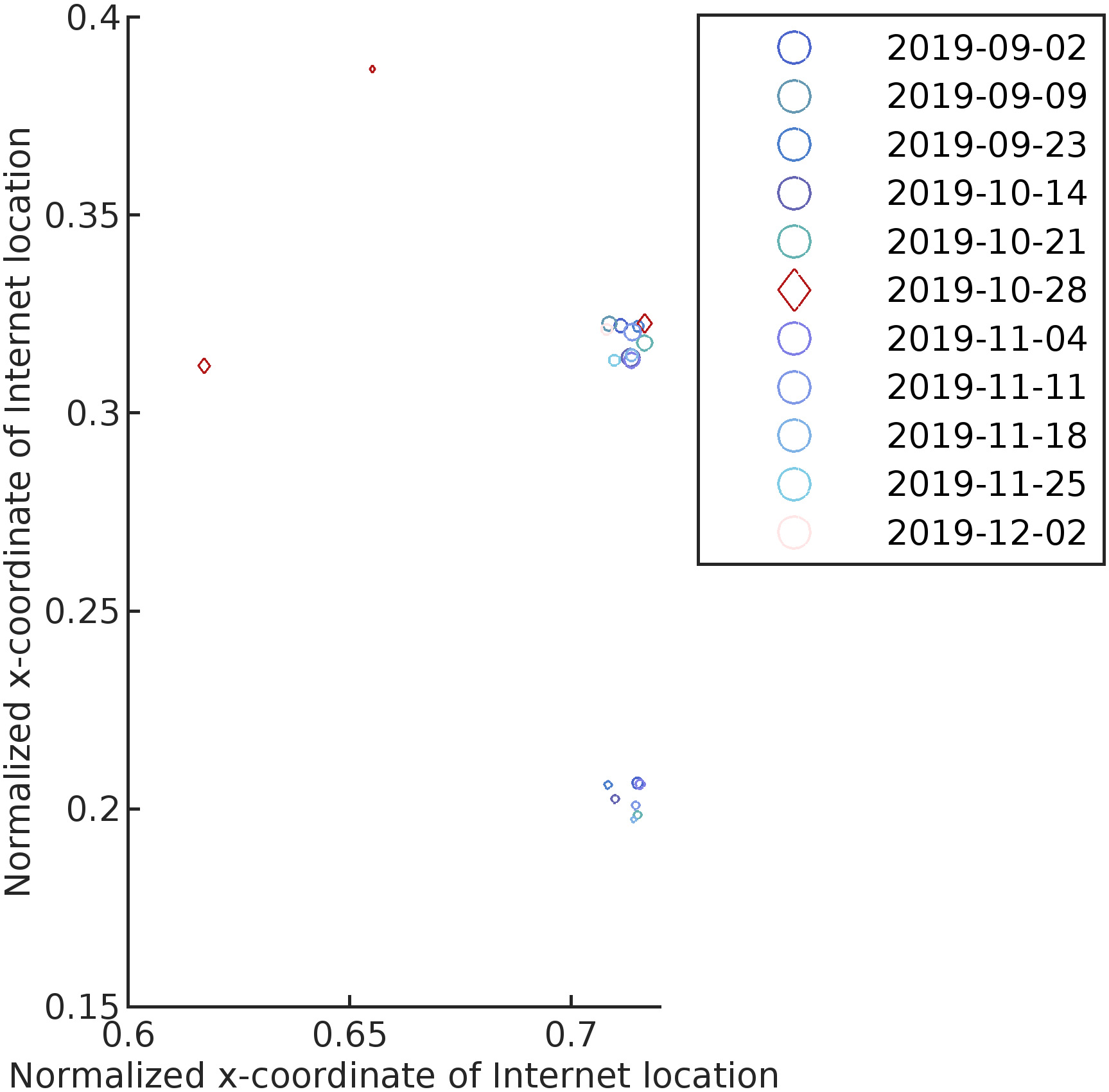

As it can be seen from Fig. 2, provided that there is a sufficient trajectory sequence, User_3 basically visited two locations between 2 and 4 pm on Mondays. On October 28th, two additional locations were visited. Compared to other Monday afternoons in the same time period, this trajectory is indeed abnormal.

Next, we analyze the abnormal trajectory pattern of the group. Take one of the filtered abnormal trajectories as an example, trace the source to the corresponding User A and date. Select User B who is in the same major and class with high similarity and extract one-day spatial-temporal trajectory data of the two people. For convenience, we divide one day into 6 time periods, each time period contains 4 hours. The number of places visited by Users A and B during each time period in this day is shown in Fig. 3. Figure 4 shows the number of Internet loggings generated by two users over time periods of the day.

Figure 3.

The number of places visited at various times on the same day.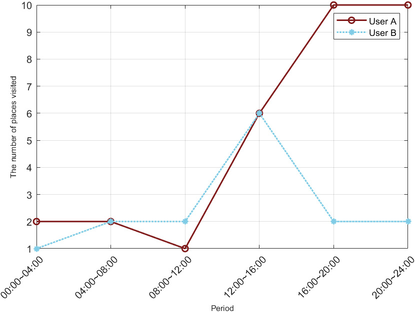

Figure 4.

The number of log records generated by going online in a day.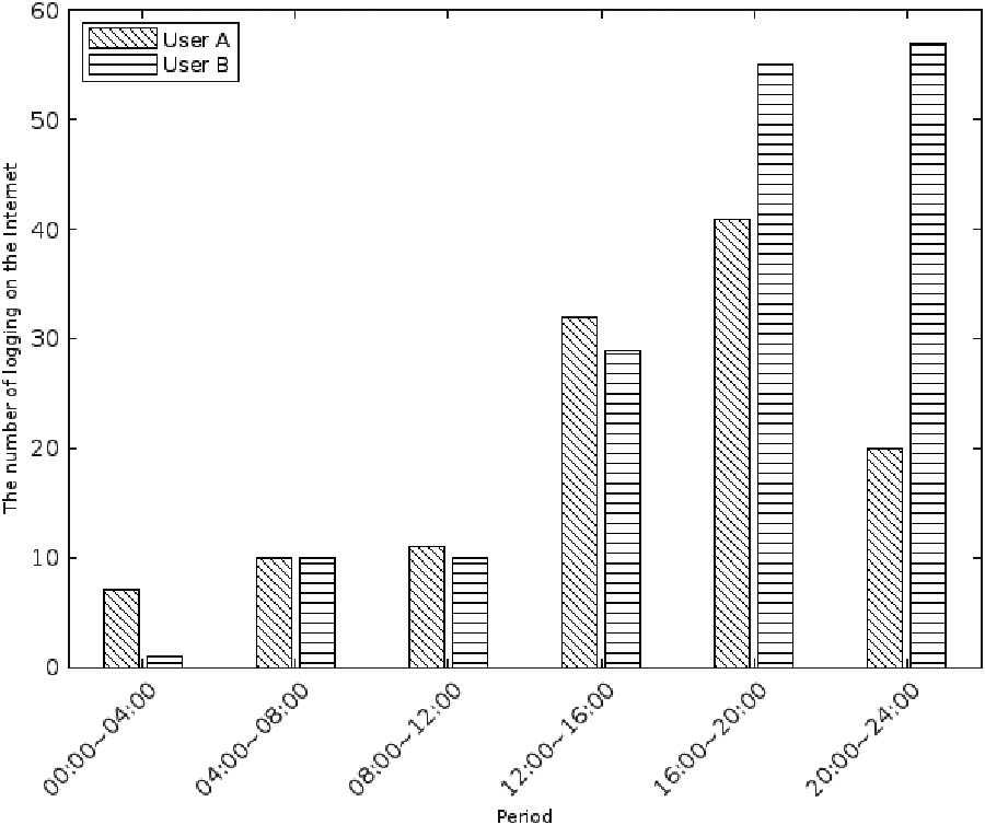

Figure 5.

Distribution of Internet locations in 16:00 to 20:00 and 20:00 to 24:00.

As can be seen from Fig. 3, there is a significant increase in the number of places visited by User A during the period 16:00–20:00 and 20:00–24:00. Based on the number of loggings in Fig. 4, both users surf the Internet at a high frequency during two periods, so we can rule out error detection due to too little data.

We can also refer to the user’s individual trajectory anomaly detection analysis method, to map out two users s in 16:00 to 20:00 and 20:00 to 24:00 two time periods online location distribution as shown in Fig. 5.

In Fig. 5, four different color and shape legends represent User A and B two different time periods. It is easy to see that User A’s Internet locations visited some other locations in addition to overlapping with some of User B’s locations. The interference factor of signal strength from different access points is excluded. It can be determined that User A’s trajectory on this day is indeed abnormal.

Therefore, the MSTDSNN-SC algorithm for spatial-temporal trajectory anomaly detection proposed in this paper is reasonable and effective. It should be aware that the results of the above-mentioned anomaly detection analysis are only to provide reference information for relevant campus managers and play a role in decision support. Whether to pay more attention to a certain student based on the test results still requires school administrators to make a choice based on the specific real situation.

6. Results

This paper introduces a method for abnormal detection based on the spatial-temporal trajectory extracted from the user’s Internet records. This method takes full account of the characteristics of space-time track data and measures the correlation between trajectories from the two dimensions of time and space. We propose corresponding improvement measures for other defects of the spectral clustering algorithm, which can be used for anomaly detection of spatial-temporal trajectories. Specifically, first of all, we improve the accuracy of spatial-temporal similarity measurement by introducing covariance scale threshold, spatial scale threshold, and location popularity. Secondly, we Skillfully use the PCA algorithm to avoid the trouble of manually selecting the number of feature vectors. Finally, we applied the MSTDSNN-SC algorithm to the ISST dataset and GSST dataset respectively and the rest 10 algorithms for comparison experiments. The experimental results show that the MSTDSNN-SC algorithm performs well in the evaluation of SI, DB, CH and DVI metrics. In particular, the experimental results are very close to 1 in the evaluation of the silhouette index, which has a fixed interval from $-$ 1 to 1.

Considering the evaluation performance of the four metrics as well as the reasonableness of the number of clusters and the number of detected outlier points, the clustering results obtained by the MSTDSNN-SC algorithm are reliable. What’s more, after visual analysis and validation, the screened outlier data also do have anomalies.

References

Ester

Kriegel

H.-P.

Sander

and Xu

, A Density-Based Algorithm for Discovering Clusters in Large Spatial Databases with Noise, 1996. pp. 226–31.

Bai

Lei

Zhu

Sun

et al., Traffic Anomaly Detection via Perspective Map based on Spatial-temporal Information Matrix, CVPR Workshops; 2019.

Yamanishi

Takeuchi

J.-I.

Williams

and Milne

, On-line unsupervised outlier detection using finite mixtures with discounting learning algorithms, Data Mining and Knowledge Discovery 8(3) (2004), 275–300.

Ferreira

Klosowski

J.T.

Scheidegger

C.E.

and Silva

C.T.

, Vector field käŽšmeans: Clustering trajectories by fitting multiple vector fields, Computer Graphics Forum; 2013: Wiley Online Library.

Navarro

Martin de Diego

Fernandez-Isabel

Ortega

and Assoc Comp

, Fusion of GPS and Accelerometer Information for Anomalous Trajectories Detection, 2019. pp. 43–8.

Z.-P.

Zhang

S.-F.

and Sun

D.-G.

, Parallel spatial-temporal convolutional neural networks for anomaly detection and location in crowded scenes, Journal of Visual Communication and Image Representation 67 (2020), 102765.

Rajasegarar

Leckie

and Palaniswami

, Hyperspherical cluster based distributed anomaly detection in wireless sensor networks, Journal of Parallel and Distributed Computing 74(1) (2014), 1833–47.

Hartigan

J.A.

and Wong

M.A.

, A K-means Clustering Algorithm: Algorithm AS 136. 281979. p. 100–8.

A.Y.

Jordan

M.I.

Weiss

, editors, On Spectral Clustering: Analysis and an Algorithm, Proceedings of the 14th International Conference on Neural Information Processing Systems: Natural and Synthetic, 2001.

10.

Frey

B.J.

and Dueck

, Clustering by Passing Messages Between Data Points, Science, 2007.

11.

Wang

Ding

and Jia

, Spectral Clustering Algorithm Based on Message Passing, Data Acquisition and Processing 34(3) (2019), 548–57.

12.

Guo

Yang

Hou

and Meng

, An Improved DBSCAN Algorithm Based on Similarity Measures, Mathematics in Practice and Theory 50(6) (2020), 164–70.

13.

Wen

Tong

and Tan

, Spectral Clustering Algorithm Based on Local Covariance Matrix, Computer Engineering and Applications 55(14) (2019), 148–54.

14.

Natali

Puri

Kenny

J.M.

Torre

and Rallini

, Microstructure and ablation behavior of an affordable and reliable nanostructured Phenolic Impregnated Carbon Ablator (PICA), Polymer Degradation and Stability 141 (2017), 84–96. doi: 10.1016/j.polymdegradstab.2017.05.017. PubMed PMID: WOS:000404500400012.

15.

Mao

Jin

Zhang

and Zhou

, Anomaly Detection for Trajectory Big Data: Advancements and Framework, Journal of Software 28(1) (2017), 17–34. PubMed PMID: CSCD:5926435.

16.

Ding

Huang

Wang

and Wang

, Inventors; Univ China Civil Aviation, assignee, Time sequence based multi-dimensional distance clustering abnormal detection method, involves clustering abnormal track with normal track, and selecting correct rate, precision rate and recall rate to evaluate clustering algorithm patent CN110490264-A.

17.

Chalapathy

and Chawla

, Deep learning for anomaly detection: A survey, arXiv preprint arXiv:190103407. 2019.

18.

Jiang

Cai

Wang

and Chen

, Trajectory-based anomalous behaviour detection for intelligent traffic surveillance, IET Intelligent Transport Systems 9(8) (2015), 810–6.

19.

Zhang

Luo

Sun

and Sun

, A Framework of Abnormal Behavior Detection and Classification Based on Big Trajectory Data for Mobile Networks, Security and Communication Networks 2020 (2020). doi: 10.1155/2020/8858444. PubMed PMID: WOS:000607929600004.

20.

Hui

Peng

Jing

Zhou

and Jia

, Driving Behavior Clustering and Abnormal Detection Method Based on Agglomerative Hierarchy, Computer Engineering 44(12) (2018), 196–201. PubMed PMID: CSCD:6386148.

21.

Ding

Wang

and Li

, Anomaly Detection In Large-Scale Trajectories Using Hybrid Grid-Based Hierarchical Clustering, International Journal of Robotics & Automation 33(5) (2018), 474–80. doi: 10.2316/Journal.206.2018.5.206-0061. PubMed PMID: WOS:000453596100004.

22.

M.X.

Ngan

H.Y.T.

and Liu

, Density-based Outlier Detection by Local Outlier Factor on Largescale Traffic Data, Electronic Imaging, 2016.

23.

Wang

Peng

Han

J.-Y.

and Liu

, Density-Based Distributed Clustering Method, Journal of Software (2017).

24.

Qiang

Sun

and Deng

, Research on identification of aircraft abnormal trajectory in terminal area, China Safety Science Journal (CSSJ) 28(11) (2018), 21–7. PubMed PMID: CSCD:6423493.

25.

Liu

R.W.

Xiong

and Kim

T.-H.

, A Dimensionality Reduction-Based Multi-Step Clustering Method for Robust Vessel Trajectory Analysis, Sensors 17(8) (2017). doi: 10.3390/s17081792. PubMed PMID: WOS:000408576900095.

26.

Wang

Chen

Nie

and Li

, Detecting coherent groups in crowd scenes by multiview clustering, IEEE Transactions on Pattern Analysis and Machine Intelligence 42(1) (2018), 46–58.

27.

Wang

Liu

Chen

and Li

, Robust Rank-Constrained Sparse Learning: A Graph-Based Framework for Single View and Multiview Clustering, IEEE Transactions on Cybernetics (2021).

28.

Lian

Xiong

Lee

Feng

, editors, A Local Density Based Spatial Clustering Algorithm with Noise, Systems, Man and Cybernetics, 2006 SMC ’06 IEEE International Conference on; 2006.

29.

Ankerst

Breunig

M.M.

Kriegel

H.P.

Sander

, editors, OPTICS: Ordering Points to Identify the Clustering Structure, SIGMOD 1999, Proceedings ACM SIGMOD International Conference on Management of Data, June 1–3, 1999, Philadelphia, Pennsylvania, USA; 1999.

30.

Birant

and Kut

, Spatio-Temporal Outlier Detection in Large Databases, Journal of Computing and Information Technology 14(4) (2006), 291–7.

31.

Zhou

Ding

Luo

and Hou

, Trajectory outlier detection based on DBSCAN clustering algorithm, Infrared and Laser Engineering 46(5) (2017), 0528001-1–8. PubMed PMID: CSCD:6000360.

32.

Zhong

and Zhang

, Adaptive Multiobjective Memetic Fuzzy Clustering Algorithm for Remote Sensing Imagery, IEEE Transactions on Geoscience and Remote Sensing 53(8) (2015), 4202–17. doi: 10.1109/tgrs.2015.2393357. PubMed PMID: WOS:000351763800006.

33.

Zhang

and Wu

, Optimization and Application of Clustering Algorithm in Community Discovery, Wireless Personal Communications 102(4) (2018), 2443–54. doi: 10.1007/s11277-018-5264-x. PubMed PMID: WOS:000450597900005.

34.

Zhang

Wang

Han

and Zhou

, Fuzzy-Logic Based Distributed Energy-Efficient Clustering Algorithm for Wireless Sensor Networks, Sensors (Basel, Switzerland) 17(7) (2017). doi: 10.3390/s17071554. PubMed PMID: MEDLINE:28671641.

35.

Luxburg

, A Tutorial on Spectral Clustering, Statistics and Computing 17 (2004), 395–416. doi: 10.1007/s11222-007-9033-z.

36.

Shi

and Malik

J.M.

, Normalized Cuts and Image Segmentation, IEEE Transactions on Pattern Analysis and Machine Intelligence (2000).

37.

Bhissy

Faleet

and Ashour

, Spectral Clustering Using Optimized Gaussian Kernel Function, International Journal of Artificial Intelligence and Application for Smart Devices 2 (2014), 41–56. doi: 10.14257/ijaiasd.2014.2.1.04.

38.

Chen

and Lin

, Abnormal Trajectory Detection Method Based on BP Neural Network, Computer Engineering 45(7) (2019), 229–36, 41. PubMed PMID: CSCD:6529169.

39.

Donath

W.E.

and Hoffman

A.J.

, Lower Bounds for the Partitioning of Graphs, IBM Journal of Research and Development 17(5) (1973), 420–5.

40.

Fang

and Liu

, Spatial-temporal trajectory similarity measurement based on campus wireless network, Computer Engineering and Design 41(11) (2020), 3001–8.

41.

Vlachos

, editor, Discovering Similar Multidimensional Trajectories, Data Engineering, 2002 Proceedings 18th International Conference on; 2002.

42.

Gong

Chen

Qiang

and Jin

, Trajectory pattern change analysis in campus WiFi networks, Mobile Geographic Information Systems (2013).

43.

and Liu

, Correlation measurement of campus wireless network users based on the shortest time distance, Computer Engineering and Science 41(10) (2019), 1755–62.

44.

Peng

Zhang

, editors, Scalable Sparse Subspace Clustering, 2013 IEEE Conference on Computer Vision and Pattern Recognition; 23-28 June 2013.

45.

Zhang

Zhao

, editors, A Novel Algorithm for Detecting Spatial-Temporal Trajectory Outlier, International Conference on Computer Science & Electronic Technology; 2016.

46.

M.J.

and Ng

M.K.

, On cluster tree for nested and multi-density data clustering, Pattern Recognition 43(9) (2010), 3130–43. doi: 10.1016/j.patcog.2010.03.020. PubMed PMID: WOS:000279271800013.

47.

Liu

and Xiang

, Fast Searching Density Peak Clustering Algorithm Based on Shared Nearest Neighbor and Adaptive Clustering Center, Symmetry-Basel 12(12) (2020). doi: 10.3390/sym12122014. PubMed PMID: WOS:000602314500001.

48.

Qiu

and Xin

, Shared nearest neighbor affinity based clustering algorithm, Computer Engineering and Applications 54(18) (2018), 184-7+222.

49.

Rousseeuw

P.J.

, Silhouettes: A graphical aid to the interpretation and validation of cluster analysis, Journal of Computational and Applied Mathematics (1987).

50.

Davies

D.L.

and Bouldin

D.W.

, A Cluster Separation Measure, IEEE Transactions on Pattern Analysis and Machine Intelligence PAMI-1(2) (1979), 224–7.

51.

Calinski

and Harabasz

, A Dendrite Method for Cluster Analysis, Communications in Statistics – Simulation and Computation 3(1) (1974).

52.

Dunn

J.C.

, Indices of partition fuzziness and the detection of clusters in large data sets, 1977.

Spatial-temporal trajectory anomaly detection based on an improved spectral clustering algorithm

Abstract

Keywords

1. Introduction

2.1 Taxonomy of trajectory outlier detection technique

2.1.1 Uncertainty

2.1.2 Sparsity and skewed distribution

2.1.3 Low density value

2.2 Spatial-temporal trajectory anomaly detection based on clustering algorithm

3. Spectral clustering algorithm

4.1 Optimization of similarity measures

5. Experiments

5.1 Experimental data set and metrics

Table 1 Original data format

5.2.1 Format conversion

5.2.2 Data cleaning

5.2.3 Anonymous processing

5.2.4 Map matching

5.3 Parameter selection

Table 2 Comparison experiment parameter in ISST dataset

5.4.1 Results of ISST dataset

Table 4 Performances of clustering algorithms for ISST dataset

Table 5 Performances of clustering algorithms on GSST dataset

References

Table 1
Original data format

Table 2
Comparison experiment parameter in ISST dataset

Table 4
Performances of clustering algorithms for ISST dataset

Table 5
Performances of clustering algorithms on GSST dataset