
Abstract
We propose a new method of constructing a variable bin width histogram that can accommodate the unbalanced distribution of the samples yet retaining, as a whole, the good aspect of both equal width (EW) and equal-area (EA) histograms that are being used popularly for data visualization and analysis. We formulate this as an optimal change point detection problem in which the bin boundaries are determined by minimizing the sum of the absolute error or the squared error in each bin. The former is based on Distance Minimization (DM) and new, and the latter is based on Variance Minimization (VM) and is considered the state-of-the-art. The constructed histograms can effectively be used to detect and visualize hidden outliers/anomalies by applying the interquartile range method in each bin. The final histograms are obtained by adjusting bin boundaries and heights accordingly after removing the detected outliers/anomalies. We further propose a method to annotate the constructed bins if the data for annotation is given for each sample as a set of nominal variables, using
Introduction
Histograms have been widely used to visualize and analyze the distribution of data. They can highlight the properties of data and help improve their quality. They can be used to pre-process the data that are to be fed to other system using them, e.g., machine learning system. Histograms that divides the data into separate bins (also called buckets) have merits to naturally detect and visualize outliers within each bin as well as the data themselves, and characterize each bin by annotating it using other nominal features of the data. We focus on these aspects and propose a new method to construct outlier/anomaly-free histograms with variable bin width and visualize the constructed histogram together with the detected outliers/anomalies.
The most popular standard histogram construction method uses a fixed bin width. It is important that this bin width is set properly and various methods and indicators have been proposed for this purpose [2, 16, 18, 15, 5]. Whether the equal width histogram is appropriate or not depends heavily on the sample distribution. Data with a smooth distribution is easy and the use of an equal width histogram does not cause a problem. However, it is not appropriate to apply it to non-smooth unbalanced data in which some parts of data are very dense and its changes are abrupt from the neighbors. A simple way to cope with this shortcoming is to construct a histogram with equal area, i.e., equal sample size [2, 16]. However, we may miss some bins with zero width when there exist a large number of samples of identical values. In short, the equal width (EW) histogram works well for many real world datasets and the equal-area (EA) histogram is an alternative remedy when it does not work well. It is natural to conjecture that histograms that have variable bin width capability which is more robust than EA histograms can accommodate unbalanced datasets and perform better. Fisher [4] was the first to propose the concept of such histograms in which the bin boundaries are determined by minimizing the variance within each bin, which is referred to as Variance Minimization (VM) method in this paper. This idea is followed and investigated by [8, 9] and is now considered as the state-of-the-art.
Minimizing the variance is equivalent to minimizing the square error which is the L2 metric. This choice has been taken natural and no other metrics have been discussed. We note that the L1 metric is more robust to noise and outliers/anomalies, and conjecture that the L1 metric may work better than, if not, at least as good as, L2 metric. We thus propose to use the absolute error which is L1 metric and distance-based. This method is referred to as Distance Minimization (DM) method in this paper. We further propose to use a change point detection method to search for the best bin boundaries that can be applied to both measures for which we have abundant experience [14].
It is desirable that the constructed histograms still possess good properties of both equal width and equal area histograms. Here we mean by good properties that the widths of bins are almost the same and the numbers of samples in bins are almost the same across different bins. In fact, a bin with a too small width or a too small sample size is usually not worth analysis. We investigate how DM method differs from VM method and how these two are related to EW and EA methods, and demonstrate that these two properties are simultaneously achieved by minimizing the absolute error or the squared error of samples in each bin for its median or mean, based on the idea of combining histogram construction and clustering, which is the most important contribution in this work. In other words, our method constructs a histogram with variable bin width that 1) has a large number of narrow bins where the samples are densely distributed and drastically changes from their neighbors and a small number of wide bins where the samples are sparsely distributed, yet avoiding bins with too small widths and too small samples in them, and 2) shows a similar behavior of both equal width and equal area histograms where the changes are moderate.
The change point detection algorithm we use is applied to the samples that are arranged in ascending order of their numeric values. The algorithm minimizes a step function consisting of
In our previous paper [6], we have proposed a basic idea of the variable bin-width histogram construction with error minimization and visually compared the constructed histograms to EW histograms. In this paper, we further address outlier/anomaly detection problem because we note that outliers/anomalies that are hidden in the dataset can substantially distort the constructed histograms. Being unable to remove outliers/anomalies during the histogram construction process is one major limitation of the existing methods. Outlier/anomaly detection capability should be integrated into the histogram construction process. Evidently, we need some measure (score) to quantify their outlierness and anomality. We use the interquartile range method, which does not depend on sample distribution, to data samples within each bin of the histogram of this measure to detect them. When the samples are univariate which is the case in this paper, the histogram of the data themselves is used as the score. We then reconstruct the histogram after removing the detected outliers/anomalies. Thus, the final histogram is outlier/anomaly-free. One notable feature is that both detected outliers/anomalies and the reconstructed histogram are simultaneously visualized.
Here, outliers and anomalies are meant in general to be such data points that lie outside the main body or group of the dataset that they are part of. In this paper, we use outliers to indicate the data points which lie in the tails of a sampled distribution, e.g., data points that lie outside of 3
We occasionally omit anomaly to indicate both for the sake of simplicity, e.g., outlier-free instead of outlier/anomaly-free.
Another contribution in the previous paper is that we proposed a method to annotate each of the generated bins from a set of nominal data that may come with the numeric samples. For example, consider the case where each sample comes with the time stamp, temperature, and pressure that can characterize the sample. We can define a set of ranges/categories for each of these data and convert them to corresponding nominal data. We then compute
We did experimental studies to test the validity of the proposed method using real datasets of humidity deficit (HD) and carbon dioxide concentration (CO2), both collected from a vinyl greenhouse in operation as well as two sets of synthetic datasets, with each dataset generated from one of the three sample distributions: uniform, exponential and normal. Each dataset in the first set uses a single distribution without anomalous data and the one in the second set uses well separated two distributions of the same kind with an anomalous sample inserted in the middle. The latter is used to test both the anomaly and outlier detection capability. We show that our methods can construct histograms which simultaneously achieve two good properties of equal width and equal area. We confirm that our proposed methods can construct histograms with appropriate various bin widths that can well represent the sample distribution with a smaller bin size
Last, to make the difference from the conference paper clear, we summarize the major additions to this paper: 1) expansion of our framework to include outlier detection capability and to construct outlier-free histograms, 2) addition of datasets: another real-world dataset CO2, and three synthetic datasets, each with and without anomaly, 3) addition of the details of EA method, and reformulation of the proposed DM method and the state-of-the-art VM method as two instances of a minimization problem of general distortion function, 4) expansion of the quantitative evaluations by adding entropy analysis for the equal-sample-size property, computational efficiency with complexity analysis, homogeneity property analysis, and in depth comparative studies of EW, EA, VM, and DM methods, and 5) experimental evaluations of outlier/anomaly detection using synthetic datasets, 6) substantial expansion of the related work by summarizing it from four perspectives.
The paper is organized as follows. We describe related work in Section 2, the conventional methods in Section 3, give our problem setting and the proposed method for 1) constructing a variable bin width histogram, 2) detecting outliers within each bin and 3) selecting terms for annotation in Section 4. We report and discuss experimental results for both real world data and synthetic data in Section 5 and conclude this paper and address the future work in Section 6.
We summarize related work from four different aspects: histogram construction, clustering, change point detection, and outlier detection.
Histogram construction
Histograms measure and visualize the density of numeric variables that take continuous values. The bin widths are often set equal, the horizontal axis represents the range of sample values (bin), and the vertical axis represents the density of samples included in that range (bin). Indices that determine the number of bins or the width of bins, that is, the number of intervals needed to divide all samples into, include square root selection,2
Microsoft EXCEL uses this strategy.
Methods to construct histograms with variable bin width have been proposed [4, 16, 2], which bring the advantages of improving the robustness for noises and the accuracy of density estimation by assigning wider bins for low-density ranges and narrower bins for high-density ranges. Scott’s equal area histogram [16] adjusts the width of each bin so that each bin contains an equal number of samples. Denby and Mallows’ diagonally-cut histogram [2] is an intermediate histogram that generalizes an equal width histogram and an equal area histogram. It is obtained by dividing the samples by diagonally cutting the cumulative distribution of data. These histograms make it easier to identify peaks because the data is not over-smoothed, but at the same time, they are likely to include bins with too small widths and/or too few samples. On the contrary, the proposed method would rarely generate histograms with such extreme bins because it is based on the concept of clustering obtained by error minimization, and we can expect to have good properties of both equal width and equal area.
A series of works have been presented by Poosala and Ioannidis et al. who argued and emphasized that it is important to construct a proper histogram when estimating the size of query results in the query optimization problem in RDBS (Relational Database System). They pointed out the problem of classic histogram construction methods and defined the V-optimal histogram that minimizes the variance of the data in each bin in the histogram [8, 9]. Further, in their succeeding work [13, 12], they compared the V-optimal histogram and the histogram constructed by the existing method, and discussed the advantage and disadvantage of each histogram for artificial data with various distributions including a uniform distribution. Irpino and Romano noted that the V-optimal histogram method based on variance minimization of data in each bin is equivalent to the grouping method proposed by Fisher [4], and compared the Fisher’s algorithm with an algorithm for estimating the density distribution by piece-wise linear interpolation [10]. As mentioned in Section 1, our VM method is equivalent to the V-optimal histogram and Fisher methods in the spirit of the squared error minimization, and is implemented by using a different boundary search algorithm, i.e., change point detection algorithm. Thus, our proposed method provides a general framework that includes these two methods in that an optimal histogram can be constructed by minimizing either one of the two kinds of errors, the absolute or the squared.
Clustering is the task of grouping a set of samples in such a way that samples in the same cluster are more similar to each other than to those in other clusters. This is a rich research field and has a long history. Many different clustering algorithms have been proposed and tested for their performance. These include hierarchical clustering, centroid-based clustering, distribution-based clustering, density-based clustering, subspace clustering, and more. Constructing a histogram is considered to be a special instance of clustering samples in one-dimensional consecutive bins. Our method, which is described in Section 4, uses the absolute or the squared error of samples in each bin for its median or mean as an objective function to be minimized, and the search is made of bin’s boundaries using the method developed for change point detection [14].
We notice that our method is doing centroid-based clustering in one dimension, and is equivalent to
Change point detection
We view histogram construction as a problem of detecting changes in data. There are abundant studies on detecting changes in social media data [22, 21, 3, 1, 11, 19, 20]. In the spirit, our problem setting is related to the work by Kleinberg [11] and Swan and Allan [20]. They noted a huge volume of the stream data, tried to organize it and extract structures behind it. This is done in a retrospective framework, i.e., assuming that there is a flood of abundant data already and there is a strong need to understand it. Kleinberg’s work is motivated by the fact that the appearance of a topic in a document stream is signaled by a burst of activity and identifying its nested structure manifests itself as a summarization of the activities over a period of time, making it possible to analyze the underlying content much easier. He used a hidden Markov model in which bursts appear naturally as state transitions, and successfully identified the hierarchical structure of e-mail messages. Swan and Allan’s work is motivated by the need to organize a huge amount of information in an efficient way. They used a statistical model of feature occurrence over time based on hypotheses testing and successfully generated clusters of named entities and noun phrases that capture the information corresponding to major topics in the corpus and designed a way to nicely display the summary on the screen (Overview Timelines).
Our framework is different from these studies. We arrange samples in ascending order of their numeric values and regard this ordering as if they are time-stamped documents in stream data. We then, by regarding these numeric values as the activity levels, detect a set of intervals each of which contains activities of similar levels. For this, we use the change point detection method [14] which was originally developed to efficiently detect bursts from the observed information diffusion data and found to perform better than Kleinberg’s method. The most noticeable difference is that we summarize our detection results as a histogram with variable bin width, rather than timelines of bursty activities.
The histogram itself can be a useful means to detect changes in the data stream. Sebastião and Gama [17] proposed a method to monitor and compare histogram distributions from two different time windows in an online setting. The method uses two layer structures that fits well to construct a histogram from a high-speed data stream (Partition Incremental Discretization algorithm) and successfully detected changes in the distribution embedded in the streaming data where the KL divergence is used to measure the difference.
Outlier detection
Since a histogram represents the distribution of data, it can also be used to detect outliers. Goldstein and Dengel [7] proposed a method called HBOS (Histogram-based Outlier Score) that computes anomaly score for each instance of multivariate data assuming the independence of each variable (feature). Basically, the anomaly score of an instance is the product of the weighted anomaly score of each feature of the instance which is the inverse of its bin height in the histogram. The score is larger when the height is smaller. HBOS can detect global outliers as reliably as the state-of-the-art algorithms but it performs poorly for local outliers. It runs much faster than the cluster-based and nearest neighbor based algorithms. Our proposed method is different in two ways. First, we are not proposing a new anomaly score for multivariate variables. We propose to use the histogram of the score for both analysis and visualization, assuming that the score is available. Second, our method detects outliers by considering the score distribution within each bin, i.e. it is detecting local outliers in each bin. Evidently, when the data is univariate, the histogram of the data themselves is used as the score.
Conventional methods
We briefly revisit the conventional methods for constructing a histogram from a given set of samples described by a numeric variable,
Here
A simple way to cope with this shortcoming is to construct a histogram with equal area, i.e., equal sample size [2, 16]. For this purpose, we introduce an array denoted by
Here the width of the
A more sophisticated way to cope with these shortcomings is to construct a histogram with variable bin widths by dividing samples into
Then, from the obtained
Here
We propose new methods for 1) constructing a histogram with variable bin width which is equipped with outlier detection capability for a given set of samples represented by a numeric variable, and 2) characterizing the numeric samples in bins by annotating the bin using terms in the nominal variables if each numeric variable comes with a set of nominal variables. These two tasks are separate. If only a numeric variable is given and no nominal variables accompany it, only the histogram is constructed from the numeric variables, outliers are detected, the final histogram is obtained by removing detected outliers and adjusting bin boundaries and heights, and the annotation part is skipped.
Histogram construction
For a given data set
where
where
where the instantiation to
In what follows, we propose a unified solution method based on the change-point detection algorithm both for DM and VM methods. The overview of our algorithm is as follows.
[!t]
In Algorithm 4.1,
As mentioned above, we use a step function to minimize the sum of errors with respect to
Next, we consider the case that there exists only one change point expressed by a sample index
Evidently, we also need to minimize
In case of the absolute error, after computing
where
We can similarly compute
Now, we generalize these error functions,
Therefore, we can formalize our change point detection problem as the minimization problem of
Here the width of the
By virtue of our variable bin width histogram, we can consider adjusting the bin width by detecting the outliers and separately plotting them within each bin. The idea of this adjustment can be viewed as an implementation of our assumption that the samples within each bin should be distributed as uniformly as possible. We use interquartile range method which does not assume that the samples follow the normal distribution as a mean to detect the outliers, and apply it to the data samples within each bin separately.
Let
Thus, we can identify a set of outlier samples
Namely, in our proposed method equipped with the above outlier detection method, we adjust the bin width and the height from
We assign annotation terms for the obtained bins from a set of the nominal variables associated with the numeric variable, once the histogram has been constructed. Let
For a pair of the
In case that the
We have conducted experiments using both the real-world datasets (distribution unknown) and the synthetic datasets generated with known distributions to evaluate the proposed method, in particular, from the following five perspectives: 1) Computational efficiency (Section 5.2), 2) Equal width and equal area properties of constructed histograms (Section 5.3), 3) Homogeneity property within each bin (Section 5.4), 4) Appropriateness of visualized histograms and outlier detection (Section 5.5), and 5) Appropriateness of annotation (Section 5.6). In particular, perspectives 2) and 3) are the keys to achieving the desirable properties of the constructed histograms.
Datasets and settings
In our experiments, we used the real environmental datasets obtained from a vinyl greenhouse of a rose farmer in Japan. In this paper, we employed the humidity deficit (HD) [
where Humi and Temp represent humidity and Celsius temperature, respectively, both of which are measurable and we used their recorded values. HD values of
The Temp and Humi data are measured at every 5 min., i.e., 288 data points per day. We used the data measured from 00:00 on March 27, 2018 to 23:55 on May 7, 2018, i.e., data for 42 days, to compute HD, which amounts to 12,096 values each. The CO2 data are measured at every 10 min., i.e., 144 data points per day. We used the data measured from 00:00 on June 22, 2019 to 23:50 on October 16, 2019, i.e., data for 117 days, which amounts to 16,848 data points. We confirmed that there were no device failure, thus there were no missing values to all of the above data. We did not do any pre-processing to clean the data. Thus, the data may include the measurement noise, but we know it is small and ignored its effect. We employed the humidity (Humi), the temperature (Temp) and the time-window (Hour) at each time point as the nominal variables to annotate HD histograms. Therefore, the data used for annotation consist of the numeric value
In addition to the above real datasets, we used two sets of synthetic data based on probability distributions. The first set is based on unimodal distributions, which includes the uniform distribution on the interval [20, 80], the exponential distribution with the parameter
The other set is based on bimodal distributions, which includes a mixture of two uniform distributions on the intervals [20, 80] and [120, 180], a mixture of two exponential distributions with the parameter
According to Sturges’ formula, the appropriate number of bins for the fixed bin-width histogram becomes
Computational efficiency of our proposed method.
We report the computational efficiency of our DM and VM methods. Figure 1 shows the results of processing time, where Fig. 1(a)–(c), correspond to the real, synthetic unimodal, and synthetic bimodal datasets, respectively. Our programs are written in C, and run on a computer with Xeon X5690 3.47 GHz CPUs using a single thread within a 192 GB main memory capacity.
From the experimental results, we see that the processing times increase almost linearly with respect to
Evaluation in terms of equal width property.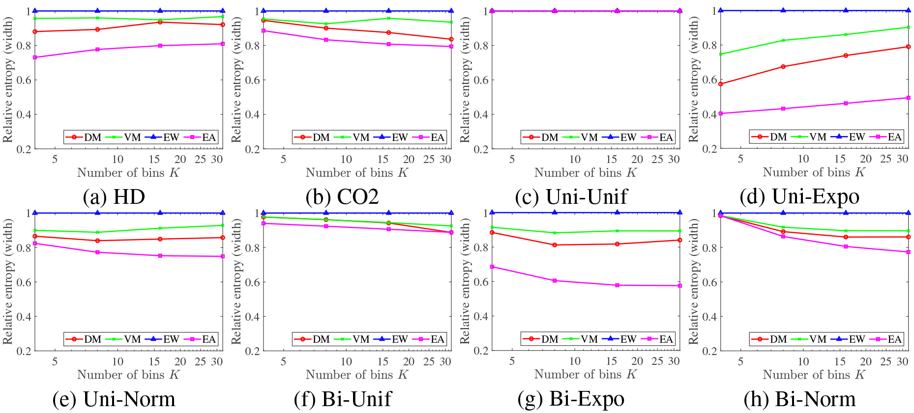
Evaluation in terms of equal sample size property.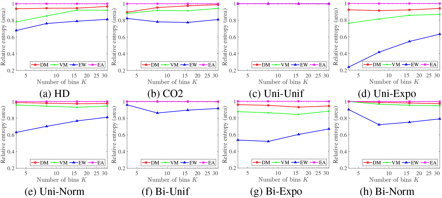
We show to what extent our histograms have the equal width and the equal area properties for various data distributions. We compute the entropy for the width of each bin for the constructed histogram
where
The result of quantitative evaluation based on the relative entropy of Eq. (19) is shown in Fig. 2, where the horizontal and the vertical axes stand for the number of bins and the relative entropy
Constructed histograms are not exactly the same because of the limited sample size (10,000 samples).
Similarly, in order to quantitatively confirm the equal area property, which means that the samples are not assigned to particular bins very unevenly, we compute the relative entropy for the number of samples in each bin defined by the following equation for the constructed histogram
The result of quantitative evaluation based on the relative entropy of Eq. (20) is shown in Fig. 3, where the horizontal and the vertical axes stand for the number of bins and the relative entropy
Each proposed entropy is a good measure to assess the intended property. EW histogram has the lowest entropy for size (Eq. (20)) and EA histogram has the lowest entropy for width (Eq. (19)), while DM and VM histograms are in between with DM higher and closer to EA and VM higher and closer to EW. This holds for both the real and the synthetic data. In summary DM and VM methods have both the equal width property and the equal-area property. DM method is closer to EA method and VM method is closer to EW method.
Evaluation of histogram based on mean absolute error.
Evaluation of histogram based on mean squared error.
We want samples with similar values to be allocated into the same bin and report to what extent this is true. For this purpose we evaluate both the mean absolute error MAE from its median
Clearly, the errors
From these figures, we see that the error decreases as the number of bins increases, which we can expect because a larger number of bins implies more homogeneous samples in each bin for all the methods. Naturally, the best result for MAE is attained by DM method and for MSE by VM method, but the difference between DM and VM is small for both MAE and MSE. Overall, the errors in EW and EA are much larger than the errors in DM and VM for both MAE and MSE. EW is the worst for MAE and EA is the worst for MSE. This supports the observation that DM is closer to EA and VM is closer to EW. We further observe that the errors in EA is less sensitive to the number of bins than the others. Here again, we confirm that all four methods give the same result in the case of Uni-Unif. The most important observation is that very roughly speaking, the number of bins of DM and VM methods that is needed to give the same error of EW and EA methods is about half in the range of
From this experiment, we confirm that the proposed method can construct variable bin-width histograms that represent the sample distribution much better than the standard equal width histogram and equal sample size histogram with the same number of bins when the sample distribution is not uniform. Said differently, the proposed method needs about the half number of bins of the conventional EW and EA methods to obtain histograms of the same performance. We will see this in the visualization results.
In the above discussion the error we considered is the total error summed over all bins. We did not assume a target homogeneity. If we do, we can evaluate binwise error and if there are bins that do not satisfy the target, we can increase the number of bins and reconstruct a histogram until all bins satisfy the requirement.
Here we report how the histograms constructed by the four methods look like, how the results in Sections 5.3 and 5.4 are realized in histograms and how the embedded outlier detection works. To save space and sharpen our discussion, we selectively choose and focus only on the informative results from among all the combination of all the variables (real, synthetic unimodal, synthetic bimodal), all the different numbers of bins, and cases with and without outlier detection. We choose the results of
Histograms without outlier detection for HD.
Histograms with outlier detection for HD.
Histograms without outlier detection for CO2.
Histograms with outlier detection for CO2.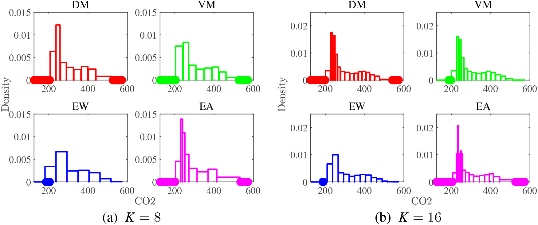
We show the visualization results of histograms for the real datasets in Fig. 6 to Fig. 9. Each variable comes with two sets of the results, one without outlier detection and the other with outlier detection, and they are arranged in pair. HD has a dense region around HD
In summary, the results obtained by the real data confirm that the proposed DM and VM methods work as intended. The drawback of EW method is clear. Using fixed-size bins, i.e., same resolution throughout the whole bins, has problems. Increasing
Histograms with outlier detection for Bi-Unif.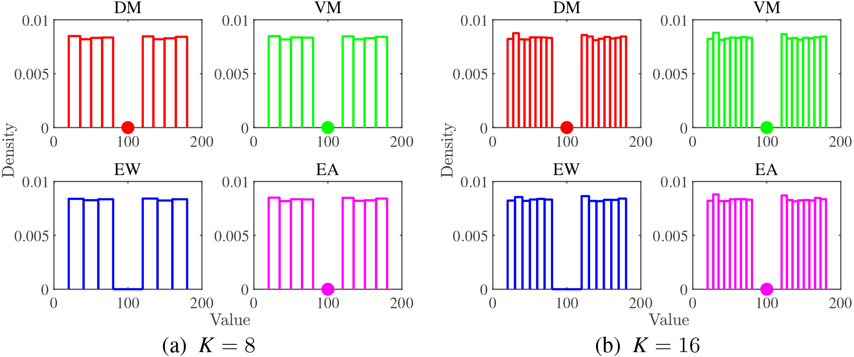
Histograms with outlier detection for Bi-Expo.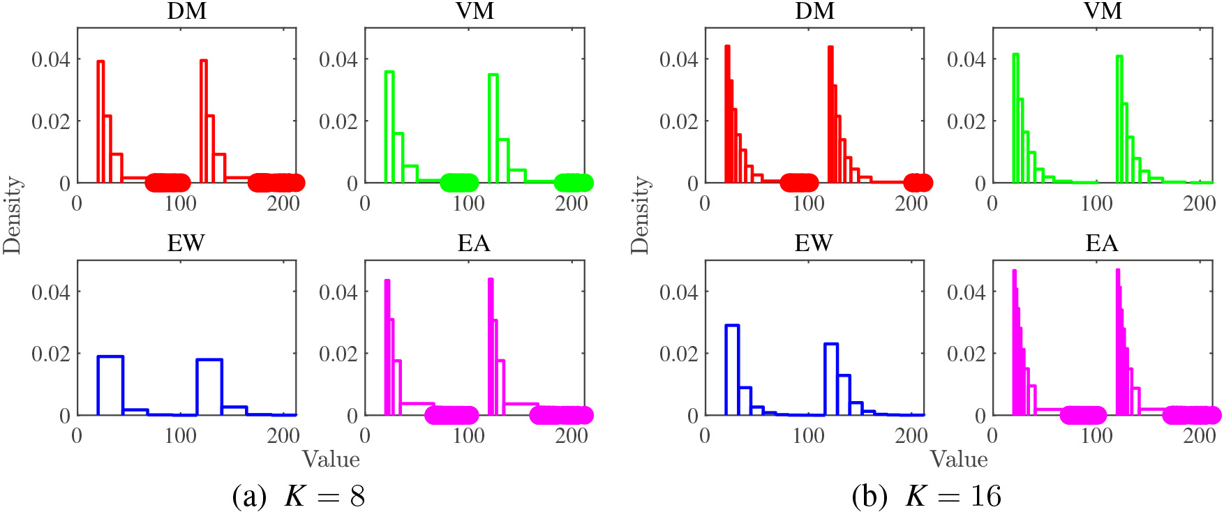
Histograms with outlier detection for Bi-Norm.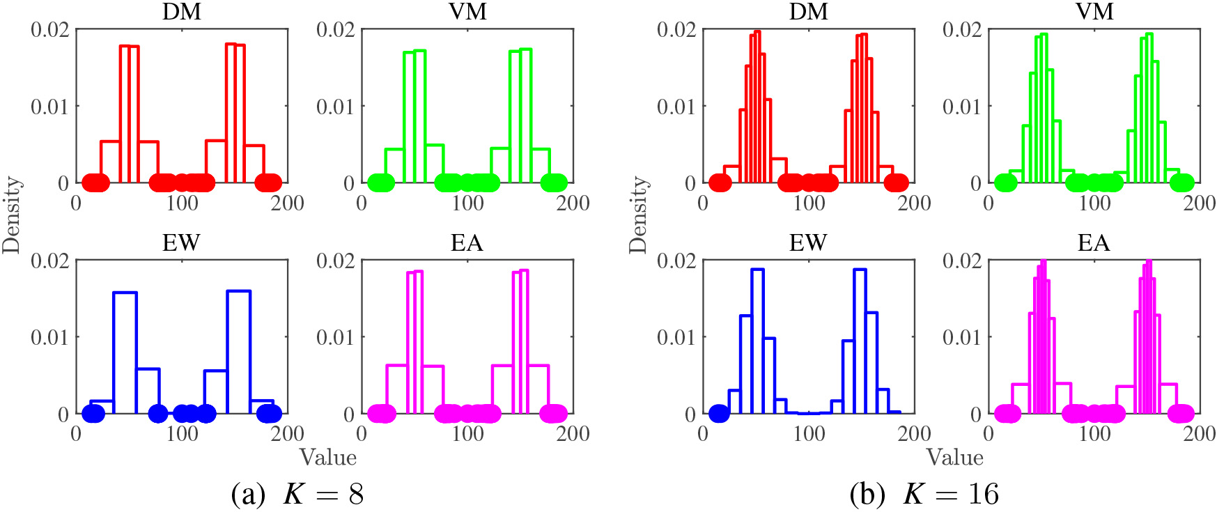
Next, we move to report the results of the synthetic datasets. Unimodal datasets are easy to analyze and interpret. What we observed in the histograms of the real dataset appears in a more understandable way, and the histograms of the bimodal dataset also have similar features of the histograms of the unimodal dataset. Thus, we focus on the bimodal dataset. The results are shown in Fig. 10 to Fig. 12. The bimodal datasets have anomalous data sample in the middle. We expect that DM and VM methods can successfully detect this anomaly in the middle as well as the outliers in the tails.
Annotation terms of each bin (
Figure 10 shows the histograms for the Bi-Unif data. As predicted, all the methods construct histograms that contains almost the same number of samples in each bin for the two regions where we have data, regardless of the number of bins
In summary, the results obtained by the synthetic datasets reconfirm the results obtained by the real datasets. We can conclude that both DM and VM methods encompass good properties of the existing EW and EA methods and accommodate to visualize the data distribution by a histogram with variable bin width using less number of bins. DM method is slightly better suited for outlier detection than VM method due to the difference in sensitivity of the mean and the median to the outliers.
In the final experiment, we report the results of characterizing the constituent samples for each bin in the histogram and evaluate whether the terms selected are appropriate for this purpose. We show this for only the HD dataset for which we know the respective categorical data. Each sample comes with
The
We note that from the definition of HD of Eq. (17), HD is negatively correlated to Humi, more sensitive than Temp, and independent of Hour. It is thus natural to observe that the majority of terms is Humi. If we pick Humi and see how it is distributed with respect to the bin ordering, i.e. the 1st bin to the 8th bin, we notice that it is arranged in descending order almost perfectly for all the methods. Exceptions are the 8-th bin in EW method where no Humi is annotated and the 1st bin in VM and EW method where no Humi90-100 (highest humidity) is annotated. The reason why EW method missed annotation in the 8th bin is that no meaningful statistical test is made because the number of samples in this bin is very small as is evident in Fig. 6(a). Similarly, the reason why EW method missed Humi90-100 in the 1st bin is that the number of samples in this bin is many and buried in many samples, and the statistical test did not pick it in the top 20 list. All the terms from Humi20-30 to Humi90-100 are annotated appropriately for bins in DM and EA methods. As we mentioned before, EA has its inherent problem of possible undrawn bins. Considering all these, we would say that the terms selected for annotation by both DM and VM methods are interpretable and reasonable. VM is slightly worse than DM. This can be explained by the observation in Section 5.3, i.e.,VM is closer to EW.
Conclusion
We addressed the problem of constructing histograms with variable bin widths by viewing the task of histogram construction as a kind of one-dimensional clustering problem and solved this as an error minimization problem. The total error is defined as the double sums of the difference of each individual sample value from the centroid value over all the samples in each bin and over all the bins. We used two error criteria: the absolute error and the squared error. The absolute error criterion enforces the centroid to be the sample median and the squared error criterion to be the sample mean. Optimal bin boundaries are obtained by an efficient greedy local improvement search which was developed to solve the change point detection problem. This naturally results in a set of bins, each containing as many homogeneous samples as possible. This formulation ensures that the optimal solution converges to equal width bins and equal sample size bins when the sample distribution is completely uniform and homogeneous. Thus, the constructed variable bin-width histogram has good properties of the standard equal width and equal area histograms when the data distribution is smooth, and constructs bins with small width for the dense region and bins with large width for the sparse region. We attempted to use the constructed histogram to detect and visualize anomalies and outliers that are hidden in the dataset. For this, we used the interquartile range method that does not assume the type of data distribution and applied it to data points within each bin of the histogram. In this paper, we dealt with univariate data. When the data are multivariate, we first compute a measure (score) of anomality and outlierness for each data point and construct a histogram for this measure, to which the same method can be applied. We further proposed a method to annotate the constructed bins for samples which comes with data for annotation as a set of nominal variables. For this, we used
We applied our method to the real datasets of humidity deficit and carbon dioxide concentration which are collected from a vinyl greenhouse in operation as well as to two different sets of three synthetic datasets, with each dataset generated from one of the three distributions (uniform, exponential and normal). Each dataset in the first set uses a single distribution without anomalous data and the one in the second set uses well separated two distributions of the same kind with an anomalous data point in the middle, and experimentally confirmed that 1) both DM and VM methods can construct histograms efficiently with the computational complexity of O(NKT) where
As a future task, we plan to conduct more experiments to see that the proposed DM method can perform well for various types of datasets in other domains, e.g., the educational field, including those with multivariate data, compare the performance with EW, EA and VM methods, and investigate in which situations DM method works better or worse than VM method. There are many factors we have to consider. These include whether domain knowledge help improve the outlier/anomaly detection capability and how noise and missing values of data samples affect the final histogram. We also plan to extend the method to be able to apply to continuously coming streaming data. Further theoretical study to find the optimal number of bins for the variable bin-width histogram is yet another important future work.
Footnotes
Acknowledgments
This work was partly supported by JSPS Grant-in-Aid for Scientific Research (C) (No. 18K11441). We thank Mr. Kiyoto Iwasaki of the Industrial Research Institute of Shizuoka Prefecture, and Prof. Seiya Okubo of the University of Shizuoka for providing and consolidating the agricultural environmental datasets.