SARW: Similarity-Aware Random Walk for GCN

Abstract

Graph Convolutional Network (GCN) is an important method for learning graph representations of nodes. For large-scale graphs, the GCN could meet with the neighborhood expansion phenomenon, which makes the model complexity high and the training time long. An efficient solution is to adopt graph sampling techniques, such as node sampling and random walk sampling. However, the existing sampling methods still suffer from aggregating too many neighbor nodes and ignoring node feature information. Therefore, in this paper, we propose a new subgraph sampling method, namely, Similarity-Aware Random Walk (SARW), for GCN with large-scale graphs. A novel similarity index between two adjacent nodes is proposed, describing the relationship of nodes with their neighbors. Then, we design a sampling probability expression between adjacent nodes using node feature information, degree information, neighbor set information, etc. Moreover, we prove the unbiasedness of the SARW-based GCN model for node representations. The simplified version of SARW (SSARW) has a much smaller variance, which indicates the effectiveness of our subgraph sampling method in large-scale graphs for GCN learning. Experiments on six datasets show our method achieves superior performance over the state-of-the-art graph sampling approaches for the large-scale graph node classification task.

Keywords

1. Introduction

In recent years, graph representation learning [1, 2, 3] has received growing attention in machine learning. Graph Neural Network (GNN) [4, 5, 6] has achieved great success in various classification tasks on graph data. Graph Convolutional Network (GCN) [7, 8] extends the classic Convolutional Neural Network (CNN) to graph-structured data. Note that CNN can deal with regular data, such as images and text, but fails to handle graph-structured data, e.g., social networks. Recently, many works [9, 10, 11] have studied the GCN for graph-structured data. Graph convolution is essentially different from conventional convolution. To be specific, the GCN updates the representation of the current node by aggregating the information of its neighbor. For example, Kipf et al. [12] used a convolution-like operation to aggregate features of all adjacent nodes of each node and performed linear transformations to generate a new feature representation of each node. However, most existing methods have focused on shallow-layer GCN and small-scale datasets. Scaling GCN to deeper layers of GCN is very challenging in large-scale graph data learning. The main problem is the neighbor explosion phenomenon when aggregating the node information, which makes the algorithm complexity high and the GCN training time too long.

Many graph sampling algorithms [13, 14, 15] have been proposed to reduce the training cost of GCN, such as node sampling, layer sampling, subgraph sampling, etc. Specifically, Hamilton et al. [16] proposed a node-wise sampling method, and Zou et al. [17] proposed a layer-wise sampling approach. However, the neighborhood expansion problem still exists. The neighbor explosion problem means that when considering higher-order neighbors or the graph scale growth, the recursive neighbor aggregation will lead to a sharp increase in the number of neighbors. It makes an exponential relationship between time complexity and graph size or GNN depth [18, 19]. More recent subgraph sampling methods have been proposed to avoid the neighbor explosion [20, 19, 21]. Zeng et al. [20] adopted a graph-wise sampling scheme to sample subgraphs for mini-batch training. They proposed four sampling algorithms, i.e., random node-based sampler, random edge-based sampler, simple random walk-based sampler (SRW), and multi-dimensional random walk-based sampler, among which the SRW performs best in their experiments. However, the above-mentioned sampling methods did not consider the features of nodes in the design of sampling probabilities. To bridge this gap, we propose a new subgraph sampling method, namely, Similarity-Aware Random Walk (SARW)-based sampling for training GCN with large-scale graphs.

The proposed SARW sampling strategy considers the similarity between the current node and the next node using both features and degree information. In addition, the SARW merges both the similarity and dissimilarity between nodes, which can adjust the impact of similarity by a parameter $\alpha$ . When $\alpha$ is larger, the feature similarity will be considered more in the selection of the next node; when $\alpha$ is smaller, feature dissimilarity will be considered more. The parameter is determined via a data-adaptive method in practice. In the training step, subgraphs are sampled from the entire graph with SARW, and a normalization technique is used to eliminate bias. At each iteration, a completed GCN is constructed from subgraphs rather than edges or nodes across GCN layers. Compared with SRW in GraphSAINT [20], the proposed SARW can obtain reliable subgraphs and has a much faster training speed. The subgraphs from the SARW sampling method can reasonably describe the full graph, which leads to better performance in GCN learning. Additionally, we proposed the simplified SARW (SSARW), which does not consider node features in sampling, and the parameter $\alpha$ is zero. The next node with fewer identical neighbors to the current node has a higher probability of being sampled by SSARW.

We evaluate our proposed approach on six large-scale graph datasets and explore the influence of the number of sampling nodes for model training. We also study the training time of our method and the training efficiency for different depths of GCN in our method. Experiments present that our method achieves superior performance over the state-of-the-art sampling methods. The node number change in the sampled subgraph has a smaller impact on our model than SRW within GraphSAINT, which indicates that our method is stable and effective. Our source code is available on the GitHub website.1

¹
https://github.com/houlinlinvictoria/SARW.

GCN faces many challenges when applied to the real world, such as node neighbor explosion, memory limitations, hardware limitations, and reliability issues. To address these challenges, subgraph sampling can be used in various fields, including social networks, recommendation systems, industrial applications, and biomedical research. For instance, subgraph sampling can aid in predicting and recommending commodities on e-commerce platforms like Amazon and Taobao, as well as identifying user patterns on social networking sites such as Reddit, Yelp, and Weibo.

The main contributions of our work are as follows:

•

A new subgraph sampling method, namely, similarity-aware random walk (SARW), is proposed for GCN learning on large-scale graphs. In the GCN training stage, we use the mini-batch training strategy and the normalization technique to reduce the sampling bias.

•

Under some mild conditions, our proposed sampling method, the simplified SARW (SSARW), is unbiased towards node representations for GCN training. The corresponding variance is much smaller than that of SRW in GraphSAINT. The effectiveness of our subgraph sampling algorithm for GCN learning is demonstrated from the theoretical aspect.

•

Experiments are conducted on six large graph datasets for node classification tasks. Results show that our SARW outperforms the state-of-the-art sampling methods in F1 scores. In addition, we study the effects of both the number of nodes in a sampled subgraph and the weight $\alpha$ in SARW. We also study the training time of our method compared with GraphSAINT-SRW and the training efficiency for different depths of GCN in our method.

2. Related work

GNN has been successfully applied to various real-world domains, such as social media [22, 23], recommender systems [24, 25], text classification [26, 27], graph classification [28], node classification [29], link prediction [30], community detection [31, 32], computer vision [33], etc. GCN [29, 34] is powerful and effective in dealing with graph data, and can learn representations of nodes with desirable performance. Bruna et al. [35] first proposed the application of an improved convolutional neural network to graph data. In recent years, researchers [36, 37] have proposed some convolutional neural networks for graphs. For example, Kipf et al. [12] proposed accelerating graph convolution calculations based on Chebyshev expansion. However, these methods can only deal with relatively small datasets, which are difficult to analyze large-scale graphs. The graph sampling technique [15, 38, 39] has been designed to learn large-scale graphs with GCN. There are mainly three kinds of graph sampling methods, i.e., node-wise sampling [40, 16], layer-wise sampling [41, 17] and graph-wise sampling [18, 20].

Hamilton et al. [42] conducted graph convolutions on a part of nodes in the neighborhoods to reduce the computational burden. Node-wise sampling is conducted only on a batch of nodes instead of the entire graph. Chen et al. [43] proposed layer-wise sampling to tackle the over-expansion of neighborhoods, where the nodes in each layer are only directly connected to the nodes in the next layer. But, the neighborhood expansion problem still exists using node-wise sampling and layer-wise sampling. Therefore, Zeng et al. [44] and Chiang et al. [18] performed mini-batches from subgraphs, which were obtained by graph-wise sampling. Zeng et al. [21] designed a graph sampling method to maintain the connectivity between the mini-batch of nodes. Chiang et al. [18] performed a preprocessing step, which calculated non-overlapping clusters of a graph.

More recently, Zeng et al. [20] studied different sampling schemes for subgraphs that perform well. Moreover, Cong et al. [39] proposed a variance reduction strategy with a fast convergence speed. Hasanzadeh et al. [38] proposed a unified graph neural network architecture similar to the Bayesian GNNs. More recent subgraph sampling methods have been designed [19, 21]. Bai et al. [19] proposed a subgraph-based ripple walk training framework for the deep and large graph neural network. Zeng et al. [21] use a deep GNN to pass messages within a localized shallow sampled subgraph to improve both the GNN efficiency and accuracy. However, many works ignored the important information when designing sampling probabilities, that is, the features of nodes and common neighbor nodes. Our sampling method is more effective and stable than Zeng et al. [20]. Generally, there are two ways to learn GCN, namely, transductive learning [45, 46] and inductive learning [42, 20]. Note that our proposed SARW is suitable for both of them and uses inductive learning in this paper.

3. Methodology

In this section, we will introduce the proposed method in detail. We propose a novel and general random walk method SARW for GCN with large-scale graphs, and SARW has several variants according to the different parameter $\alpha$ and similarity function. Advantages of our method contain that the proposed method captures node similarity using both feature and common neighbor information, which addresses the problem of aggregating too many neighbors and ignoring node features present in existing sampling methods. We consider additional factors, and our algorithm takes into account that similar nodes may have the same label, resulting in higher accuracy compared to other sampling methods. Furthermore, our method allows for theoretical derivation of the sampling probability, which is a significant advantage. The weaknesses of our method contain that the proposed sampling method can be performed relatively quickly, but it only considers the first-order neighbors of each node during the sampling process. Therefore, it does not take into account the potential influence of distant nodes, which may also have the same label and similar attributes. Therefore, in the future, we will study these issues.

The SRW method is simplistic and does not take full advantage of the node attribute information. In contrast, our proposed sampling method incorporates feature information, degree information, and common neighbor set information to design the sampling probability node expression between adjacent nodes. We also introduce a cosine function to calculate the similarity index between two adjacent nodes, which captures the similarity between nodes and describes the relationship between a node and its neighbors. During the GCN training stage, we use the mini-batch training strategy and normalization techniques to reduce the sampling bias and improve the accuracy of the training.

3.1 SARW

Figure 1.

An example of neighborhoods of nodes 1 and 2.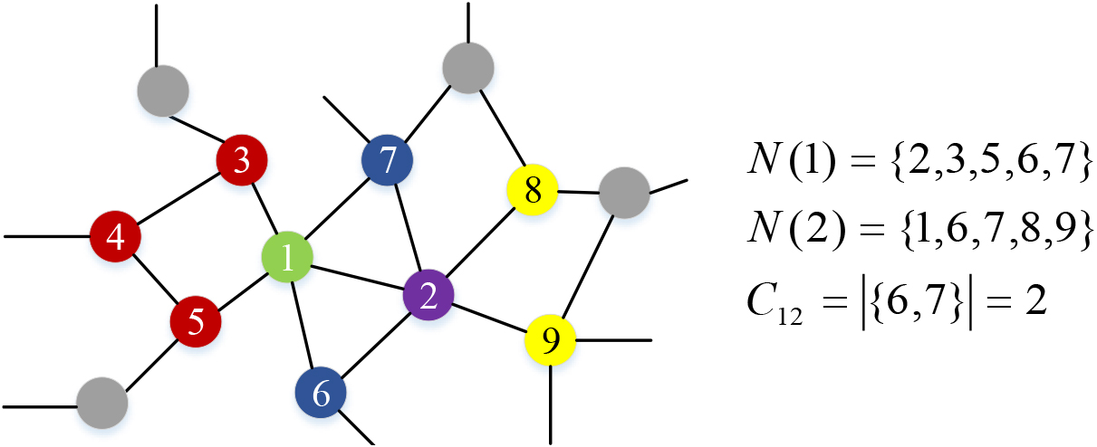

For GraphSAINT, the simple random walk (SRW) is the most effective sampling method. However, the SRW ignores the features. To alleviate the drawback of SRW, we propose a new sampling method SARW, which captures the nodes, edges, and features simultaneously. Suppose that $G(V,E)$ is an un-directed and attributed graph, where each node $v\in V$ has a $m$ -dimensional feature $x_{v}\in\mathbb{R}^{m}$ . Let $A$ and $D$ denote the adjacency matrix and the diagonal degree matrix of $G$ , respectively. This paper considers undirected and isomorphic graphs, so the neighbors of vertices in the graph have no order or direction. During GCN training, the aggregation function constructed on purpose is permutation invariance (also known as symmetry property). Permutation-invariant aggregations aim to permutate the input of an aggregate function in various orders while keeping the output of the function remains unchanged. The permutation invariance of aggregation functions ensures that GCN can be trained and applied to feature sets of vertex neighbors in any order. So in our method, we also follow the permutation invariance.

For SRW, nodes are uniformly sampled from the current node’s neighbors. Intuitively, similar samples with different labels are highly informative for training, while dissimilar samples with the same labels are also highly informative for training. To motivate the SARW, we describe the similarity between two adjacent nodes $u$ and $v$ by

$\displaystyle\textit{Sim}_{G}(u,v)=\frac{1}{f(\textit{deg}(u),\textit{deg}(v))% }\sum_{i=1}^{\lvert N(u)\rvert}\sum_{j=1}^{\lvert N(v)\rvert}{\textit{sim}(x_{% N_{i}(u)},x_{N_{j}(v)})},$ (1)

where $f(\textit{deg}(u),\textit{deg}(v))$ is a symmetric function about the degrees of $u$ and $v$ , such as $\min\{\textit{deg}(u),\linebreak\textit{deg}(v)\}$ , $\textit{deg}(u)+\textit{deg}(v)$ , $\max\{\textit{deg}(u),\textit{deg}(v)\}$ , and $\textit{deg}(u)\times\textit{deg}(v)$ , and $\textit{deg}(u)$ represents the degree of node $u$ ; $N(u)$ denotes the neighbor of node $u$ ; $\lvert N(u)\rvert$ is the size of neighbor of node $u$ ; $x_{N_{i}(u)}$ represents the input feature vector of the $i$ -th node in $N(u)$ . Note that node $u$ is in the neighborhood of $v$ and vice vase. An example of neighborhoods of two nodes is shown in Fig. 1. The neighbor of node 1 is $N(1)={2,3,5,6,7}$ and the neighbor of node 2 is $N(2)={1,6,7,8,9}$ . The $\textit{sim}(\cdot,\cdot)$ is a similarity function of two feature vectors. In this paper, $\textit{sim}(\cdot,\cdot)\in[0,1]$ is based on the following cosine function,

$\displaystyle\textit{sim}(x_{N_{i}(u)},x_{N_{j}(v)})=\frac{1}{2}\{1+\cos(x_{N_% {i}(u)},x_{N_{j}(v)})\}=\frac{1}{2}\left\{1+\frac{<x_{N_{i}(u)},x_{N_{j}(v)}>}% {\parallel x_{N_{i}(u)}\parallel\parallel x_{N_{j}(v)}\parallel}\right\},$ (2)

where $<\cdot,\cdot>$ denotes the inner product of two vectors, and $\parallel\cdot\parallel$ denotes the Euclidean norm. To adjust for the similarity between two nodes $u$ and $v$ , we propose a weighted version of $\textit{Sim}_{G}(u,v)$ for deriving probability from $u$ to $v$ ,

$\displaystyle p_{uv}=\alpha\times\textit{similarity}+(1-\alpha)\times\textit{% dissimilarity}=\alpha\textit{Sim}_{G}(u,v)+(1-\alpha)\{1-\textit{Sim}_{G}(u,v)\}$ (3)

where $\alpha\in[0,1]$ is a hyperparameter.

The main advantage of Eq. (3) is that it can describe the relationship between two nodes by feature-related statistics. Furthermore, it is more flexible for considering both the similarity and dissimilarity with the hyperparameter $\alpha$ , which is determined via a data-adaptive method in practice. Note that Eq. (3) includes three special cases:

•

Case 1: For $\alpha=0$ , then $p_{uv}=1-\textit{Sim}_{G}(u,v)$ . In this case, the similarity statistic has a negative effect on the probability from $u$ to $v$ .

•

Case 2: For $\alpha=1$ , then $p_{uv}=\textit{Sim}_{G}(u,v)$ . In this case, the similarity of features has a positive effect on the probability between nodes $u$ and $v$ .

•

Case 3: If the features are missing or not considered,2

When the feature dimension is high for some graphs, the computational complexity for SARW is relatively high.

i.e.,

x_{N_{i}(u)}=\textit{null}

, we define

$\displaystyle\textit{sim}(x_{N_{i}(u)},\ x_{N_{j}(v)})=\left\{\begin{array}[]{% ll}1,&\text{if }N_{i}(u)=N_{j}(v)\\ 0,&\text{if }N_{i}(u)\neq N_{j}(v).\\ \end{array}\right.$ (4)

In this case, the Eq. (1) is reduced to

$\displaystyle\textit{Sim}_{G}(u,v)=\frac{1}{f(\textit{deg}(u),\textit{deg}(v))% }\sum_{i=1}^{\lvert N(u)\rvert}\sum_{j=1}^{\lvert N(v)\rvert}\mathbb{I}(N_{i}(% u)=N_{j}(v))=\frac{1}{f(\textit{deg}(u),\textit{deg}(v))}C_{uv},$ (5)

where $\mathbb{I}$ is an indicator function and $C_{uv}$ represents the number of common neighbors between the node $u$ and node $v$ . As shown in Fig. 1, $C_{12}$ is 2. According to the definition of formula $C_{uv}$ , it can be seen that $C_{13}=0$ , $C_{15}=0$ , $C_{16}=|\{2\}|=1$ , $C_{17}=|\{2\}|=1$ , $C_{12}=|\{6,\ 7\}|=2$ . Assuming that the next step tends to sample node 2, starting with node 1, because the number of common neighbors between nodes 1 and 2 is two, which is greater than the number of common neighbors between node 1 and its other neighbors. Using Eq. (5) as an example, when the similarity function is proportional to $C_{uv}$ , the next step tends to sample node 2. Therefore, the walking route is $1\rightarrow 2$ . It follows that Eq. (3) is

$\displaystyle p_{uv}=\alpha\frac{1}{f(\textit{deg}(u),\textit{deg}(v))}C_{uv}+% (1-\alpha)\left(1-\frac{1}{f(\textit{deg}(u),\textit{deg}(v))}C_{uv}\right).$ (6)

[ht] : Subgraph sampling algorithm with SARWInput: Training graph $G(V,E)$ ; Sampling parameters: number of roots $r$ ; random walk length $h$ ; $\alpha$ Output: Sampled graph $G_{s}$ [1] $V_{\textit{root}}\leftarrow r$ root nodes sampled uniformly at random from $V$ . $V_{s}\leftarrow V_{\textit{root}}$ $u\in V_{\textit{root}}$ $d=1$ to $h$ Select $v$ uniformly at random from $u$ ’s neighbors. Generate a random number $p\in[0,1]$ . Compute $p_{uv}=\alpha\textit{Sim}_{G}(u,v)+(1-\alpha)(1-\textit{Sim}_{G}(u,v))$ . $p\leqslant p_{uv}$ $V_{s}\leftarrow V_{s}\cup v$ $u\leftarrow v$ $G_{s}=(V_{s},E_{s})\leftarrow$ Induce subgraph from $G$ by nodes $V_{s}$ .

In Algorithm 1, we propose a novel SARW-based subgraph sampling method to perform the large-scale graph node classification task. Because the probability distribution $p$ is complicated, we adopt the accept-reject sampling strategy. For $v\in V$ , the GCN propagation rule (the aggregate function) of the ( $l+1$ )-layer in this paper is defined as [12, 20]:

$\displaystyle x_{v}^{l+1}=\sigma\left(\sum_{u\in V}\widetilde{A}_{vu}(W^{l})^{% T}x_{u}^{l}\right),$ (7)

where $\widetilde{A}$ is the normalized adjacency matrix (i.e., $\widetilde{A}=D^{-1}A$ ), $W^{l}$ is the parameter of $l$ -layer, $\sigma$ is the activation function. $x_{v}^{l+1}$ is the representation vector of node $v$ in ( $l+1$ )-layer of GCN. After a subgraph $G_{s}=(V_{s},E_{s})$ is obtained by SARW, we consider a ( $l+1$ )-layer node $v$ and a $l$ -layer node $u$ . If $v$ is sampled (i.e., $v\in V_{s}$ ), we compute the aggregated feature of $v$ as:

$\displaystyle\zeta^{l+1}_{v}=\sum_{u\in V}\frac{\widetilde{A}_{uv}}{\beta_{uv}% }(W^{l})^{T}x_{u}^{l}\mathbb{I}_{u|v}=\sum_{u\in V}\frac{\widetilde{A}_{uv}}{% \beta_{uv}}\widetilde{x}_{u}^{l}\mathbb{I}_{u|v},$ (8)

where $(W^{l})^{T}x_{u}^{l}=\widetilde{x}_{u}^{l}$ , and $\mathbb{I}_{u|v}$ is an indicator function for $v\in E_{s}$ , i.e.,

$\displaystyle\mathbb{I}_{u|v}=\left\{\begin{array}[]{ll}1,&\text{if }e(u,v)\in E% _{s},\\ 0,&\text{if }v\in V_{s}\text{ and }e(u,v)\not\in E_{s},\\ \end{array}\right.$ (9)

where $e(u,v)$ represents the edge between $u$ and $v$ . The constant $\beta_{uv}$ is a normalization factor. Here, we set $\beta_{uv}=\frac{p_{uv}}{p_{v}}$ , where $p_{v}$ represents the probability of node $u$ being visited in the sampling algorithm.

During the training stage, our model adopts the mini-batch training strategy and the normalization technique to reduce the sampling bias [20], as follows:

$\displaystyle L_{\textit{batch}}=\sum_{v\in G_{s}}\frac{L_{v}}{\lambda_{v}},$ (10)

where $\lambda_{v}=|V\rvert\times p_{v}$ is a normalization constant, $L_{v}$ is the cross loss function value of the output layer of node $v$ , i.e.,

$\displaystyle L_{v}=-Y_{v}\ln\hat{Y_{v}},$ (11)

$Y_{v}$ is the real label of node $v$ , $\hat{Y_{i}}=\textit{softmax}(\hat{Z})$ is the prediction label, $Z$ is the output of the last layer of GCN, and the last decoder generally adopts softmax function. Therefore, The overall architecture of the proposed model based on GCN is illustrated in Fig. 2. Note that this paper focuses on the problem of graph sampling suitable for big data GCN training. The data domains used in this paper are isomorphic graphs and undirected graphs. It is well-known that GCNs work on isomorphic graphs, which are graphs with a single type of edge and a single type of node. Non-isomorphic graphs, such as heterogeneous graphs, refer to graphs with multiple types of nodes and edges. For the learning of heterogeneous graphs, heterogeneous graph neural networks are typically used.

Figure 2.

The architecture of the proposed model.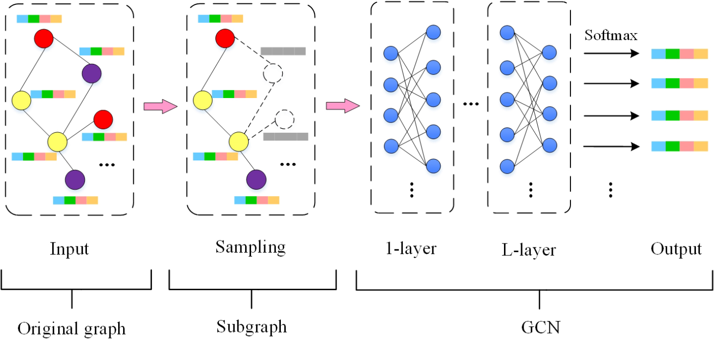

3.2 The simplified SARW

Figure 3.

An example about SRW and SSARW.

As mentioned earlier, when the dimension of node features is high, the similarity calculation for nodes is time-consumption. Therefore, a simplified version of SARW is investigated in this subsection.

In Case 3 of SARW with $\alpha=0$ , the Eq. (3) is simplified to

$\displaystyle p_{uv}=1-\frac{1}{f(\textit{deg}(u),\textit{deg}(v))}\sum_{i=1}^% {\lvert N(u)\rvert}\sum_{j=1}^{\lvert N(v)\rvert}\mathbb{I}(N_{i}(u)=N_{j}(v))% =1-\frac{C_{uv}}{\min\{\textit{deg}(u),\textit{deg}(v)\}},$ (12)

where $C_{uv}$ represents the number of common neighbors between the node $u$ and node $v$ . In this particular case, our simplified SARW is similar to the random Walk by Li et al. [47]. For notational convenience, we denote this particular case as SSARW in the remainder. Note that one particular type of the third case of Eq. (3) (i.e., in Case 3 of SARW with $\alpha=0$ ) equals SSARW.

The SSARW has a higher probability to select the next node, which has less common neighbors with the current node and a larger degree. Figure 3a and b are diagrams for SRW and SSARW, respectively (the dark lines and nodes are sampled subgraphs). Figure 3c gives an illustrative example of a two-layer GCN on the sampled subgraph with SSARW. With the same experimental settings (the same root node size and random walk length), the length of the subgraph coming from SSARW is much longer than that of SRW. Moreover, the SRW is easy to fall into a circle and visits previously sampled nodes.

Below, we conduct mathematical analysis for SSARW based on statistical sampling theory. A random walk on a graph could be viewed as a finite Markov chain in mathematics. First, we introduce some preliminaries. Let $\{X_{t}\}^{k}_{t=1}$ be the Markov chain representing the sequence of visited nodes by the sampling algorithm. Then $X_{t}\in\{u_{1},u_{2},\ldots,u_{k}\}$ , where $\{u_{1},\ldots,u_{k}\}$ is sampled node set. The stationary distribution of SRW is $\pi=\{\pi(u)\}_{u\in V}$ , where $\pi(u)=\textit{deg}(u)(2\lvert E\rvert)^{-1}$ and $\pi(u)$ represents the probability of node $u$ being visited when the random walk converges [48, 49]. The transition matrix of SRW, $[P_{uv}]_{u,v\in V}$ can be written as [50, 47]:

$\displaystyle P_{uv}=\left\{\begin{array}[]{ll}\frac{1}{deg(u)},&\text{if }v% \in N(u),\\ 0,&\text{otherwise}.\\ \end{array}\right.$ (13)

For SSARW, the transition matrix $[P_{uv}]_{u,v\in V}$ can be derived by the acceptance probability (Eq. (12)) as the following formula [47]:

$\displaystyle P_{uv}=\left\{\begin{array}[]{ll}\frac{\widetilde{p}_{uv}}{1-% \widetilde{p}_{uu}},&\text{if }v\in N(u),\\ 0,&\text{otherwise},\\ \end{array}\right.$ (14)

where

$\displaystyle\widetilde{p}_{uv}=\left\{\begin{array}[]{ll}\frac{1}{\textit{deg% }(u)}\left(1-\frac{C_{uv}}{\min\{\textit{deg}(u),\textit{deg}(v)\}}\right),&% \text{if }v\in N(u),\\ 1-\sum_{k\in N(u)}\widetilde{p}_{uk},&\text{if }v=u,\\ 0,&\text{otherwise.}\\ \end{array}\right.$

The stationary probability of node $u$ can be derived as $\pi(u)=Z\times\textit{deg}(u)(1-\widetilde{p}_{uu})$ , where $Z$ is the normalization constant. We will use $p_{u}$ to denote the stationary probability in the following sections. Note that

$\displaystyle\sum_{u\in V}\pi(u)=\sum_{u\in V}Z\times\textit{deg}(u)(1-% \widetilde{p}_{uu})=1,$

$\displaystyle Z=\frac{1}{\sum_{u\in V}\textit{deg}(u)(1-\widetilde{p}_{uu})}.$

In the following theorem, we establish the unbiasedness of node representations of SSARW-based subgraph GCN learning.

.

For SSARW-based subgraph GCN learning, let $\beta=\frac{p_{uv}}{p_{v}}$ , then $\zeta^{l+1}_{v}$ is an unbiased estimator of the aggregation of $v$ in the full ( $l+1$ )-th GCN layer, where $p_{uv}=\left(1-\frac{C_{uv}}{\min\{\textit{deg}(u),\textit{deg}(v)\}}\right)% \frac{1}{\textit{deg}(u)(1-\widetilde{p}_{uu})}$ and $p_{v}=Z\times\textit{deg}(v)(1-\widetilde{p}_{vv})$ is the probability of node $u$ being visited when the SSARW sampling algorithm converges, $Z$ is a normalization constant with $Z=\frac{1}{\sum_{u\in V}\textit{deg}(u)(1-{\widetilde{p}}_{uu})}$ , i.e., $E(\zeta^{l+1}_{v})=\sum_{u\in V}\widetilde{A}_{uv}\widetilde{x}_{u}^{l}$ .

Proof..

Under the condition that $v$ is sampled, we get the expectation of the representation of node $v$ in the ( $l+1$ )-th GCN layer as follows:

where $\textit{sample}(u,v)$ indicates nodes $u$ and $v$ are sampled, and

$\displaystyle E(\mathbb{I}_{u|v})=1\times P((u,v)\textit{ is sampled }|v% \textit{ is sampled})+0)=\frac{P((u,v)\textit{ is sampled})}{P(v\textit{ is % sampled})}.$

Then, it can be derived that

$\displaystyle E(\zeta^{l+1}_{v})=\sum_{u\in V}\frac{\widetilde{A}_{uv}}{\frac{% p_{uv}}{p_{v}}}\widetilde{x}_{u}^{l}\frac{P((u,v)\textit{ is sampled})}{P(v% \textit{ is sampled})}=\sum_{u\in V}\widetilde{A}_{uv}\widetilde{x}_{u}^{l}.$

Hence, $E(\zeta^{l+1}_{v})=\sum_{u\in V}\widetilde{A}_{uv}\widetilde{x}_{u}^{l}$ . This ends the proof. ∎

The following Theorem 2 shows that the variance of SSARW-based subgraph GCN learning is much smaller than that of SRW in GraphSAINT.

.

For SRW and SSARW on GCN learning, if $\max\left\{\frac{C_{uv}}{\textit{deg}(u),}\frac{C_{uv}}{\textit{deg}(v)}\right% \}\leqslant{\widetilde{p}}_{uu}$ , then we have a comparison about the variance of node representations, i.e., $\textit{Var}(\zeta|\textit{SSARW})\leqslant\textit{Var}(\zeta|\textit{SRW})$ .

Proof..

Let $\{X_{t}\}_{t=1}^{k}$ be the chain representing a sequence of nodes visited by the SSARW. Then $X_{t}\in S$ , where $S=\{v_{1},v_{2},\ldots,v_{n}\}$ , $E$ is the set of edges, $\lvert E\rvert$ is the size of set. So $X_{t}=\{v_{1},v_{2},\ldots,v_{n}\}$ . The transition matrix and stationary distribution of SSARW are shown above. The corresponding mini-batch loss is calculated as $L_{\textit{batch}}=\sum_{v\in G_{s}}\frac{L_{v}}{\lambda_{v}}$ in Section 3.1. Therefore, from Theorem 1, we have

$\displaystyle E(L_{\textit{batch}})=\frac{1}{\lvert\mathbb{G}\rvert}\sum_{G_{s% }\in\mathbb{G}}L_{\textit{batch}}=\frac{1}{\lvert\mathbb{G}\rvert}\sum_{G_{s}% \in\mathbb{G}}\sum_{v\in V_{s}}\frac{L_{v}}{\lambda_{v}}=\frac{1}{\lvert V% \rvert}\sum_{v\in V}L_{v},$

where $\mathbb{G}$ is the sampled subgraphs. Define $\zeta$ to be the representation of all nodes in subgraph $G_{s}$ , as follows:

$\displaystyle\zeta=\sum_{l}\sum_{v\in G_{s}}\frac{\zeta_{v}^{l}}{p_{v}}.$

So, the expectation of $\zeta$ is as follows,

$\displaystyle E(\zeta)=E\left(\sum_{l}\sum_{v\in G_{s}}\frac{\zeta_{v}^{l}}{p_% {v}}\right)=E\left(\sum_{l}\sum_{v,u\in G_{s}}\frac{\widetilde{A}_{vu}}{p_{v}% \beta_{uv}}\widetilde{x}_{u}^{l}\mathbb{I}_{v}\mathbb{I}_{u|v}\right)=\sum_{l}% E\left(\sum_{v,u\in G_{s}}\frac{\widetilde{A}_{vu}}{p_{v}\beta_{uv}}\widetilde% {x}_{u}^{l}\mathbb{I}_{v}\mathbb{I}_{u|v}\right)=\sum_{l}\sum_{v,u\in G}% \widetilde{A}_{vu}\widetilde{x}_{u}^{l}.$

Hence, $E(\zeta)=\sum_{l}\Gamma_{l}$ , we set $\Gamma_{l}$ to represent

$\displaystyle\sum_{v,u\in G}\widetilde{A}_{vu}\widetilde{x}_{u}^{l}=E\left(% \sum_{v\in G_{s}}\frac{\zeta_{v}^{l}}{p_{v}}\right).$

Thus, in the SSARW algorithm, the sampling variance of the representation vector $\zeta$ is:

$\displaystyle\textit{Var}(\zeta|\textit{SSARW})=\textit{Var}\left(\sum_{l}\sum% _{v\in G_{s}}\frac{\zeta_{v}^{l}}{p_{v}}\right),$

where $p_{v}=Z\times\textit{deg}(v)(1-\widetilde{p}_{uu})$ . In a similar way, we have the sampling variance of the representation vector $\zeta$ in the SRW algorithm as follows:

$\displaystyle\textit{Var}(\zeta|\textit{SRW})=\textit{Var}\left(\sum_{l}\sum_{% v\in G_{s}}\frac{\zeta_{v}^{l}}{p^{\prime}_{v}}\right),$

where $p^{\prime}_{v}=\frac{\textit{deg}(v)}{2\lvert E\rvert}$ is the stationary probability of SRW.

Then, we can deduce that

$\displaystyle\textit{Var}(\zeta)=E\{[\zeta-E(\zeta)]^{2}\}=E\left\{\left[\sum_% {l}\sum_{v\in G_{s}}\frac{\zeta_{v}^{l}}{p_{v}}-\sum_{l}\Gamma_{l}\right]^{2}% \right\}=E\left\{\left[\sum_{l}(\sum_{v\in G_{s}}\frac{\zeta_{v}^{l}}{p_{v}}-% \Gamma_{l})\right]^{2}\right\}=E\left[\sum_{l}\left(\sum_{v\in G_{s}}\frac{% \zeta_{v}^{l}}{p_{v}}-\Gamma_{l}\right)^{2}\right]+E\left[\sum_{l_{1}\neq l_{2% }}\left(\sum_{v\in G_{s}}\frac{\zeta_{v}^{l_{1}}}{p_{v}}-\Gamma_{l_{1}}\right)% \left(\sum_{v\in G_{s}}\frac{\zeta_{v}^{l_{2}}}{p_{v}}-\Gamma_{l_{2}}\right)% \right]=E\left[\sum_{l}\left(\sum_{v\in G_{s}}\frac{\zeta_{v}^{l}}{p_{v}}-% \Gamma_{l}\right)^{2}\right]+0=\sum_{l}E\left[\left(\sum_{u,v}\frac{\zeta_{v}^% {l}}{p_{v}}\right)^{2}-2\left(\sum_{v}\frac{\zeta_{v}^{l}}{p_{v}}\right)\Gamma% _{l}+(\Gamma_{l})^{2}\right]=\sum_{l}\left\{E\left[(\sum_{v}\frac{\zeta_{v}^{l% }}{p_{v}})^{2}\right]-2E\left(\sum_{v}\frac{\zeta_{v}^{l}}{p_{v}}\right)\Gamma% _{l}+(\Gamma_{l})^{2}\right\}=\sum_{l}\left\{E\left[\left(\sum_{v}\frac{\zeta_% {v}^{l}}{p_{v}}\right)^{2}\right]-\Gamma_{l}^{2}\right\}=\sum_{l}\left\{E\left% [\sum_{v}\left(\frac{\zeta_{v}^{l}}{p_{v}}\right)^{2}+\sum_{v_{1}\neq v_{2}}% \frac{\zeta_{v_{1}}^{l}}{p_{v_{1}}}\frac{\zeta_{v_{2}}^{l}}{p_{v_{2}}}\right]-% \Gamma_{l}^{2}\right\}=\sum_{l}\left\{E\left[\sum_{v}\frac{1}{p_{v}^{2}}\frac{% p_{v}^{2}}{p_{vu}^{2}}(\widetilde{A}_{vu}\widetilde{x}_{u}^{l})^{2}\mathbb{I}_% {v}\mathbb{I}_{u|v}\right)+E\left(\sum_{v_{1}\neq v_{2}}\frac{\zeta_{v_{1}}^{l% }}{p_{v_{1}}}\frac{\zeta_{v_{2}}^{l}}{p_{v_{2}}}\right)-\Gamma_{l}^{2}\right\}% =\sum_{l}\left[\sum_{u,v}\frac{(\widetilde{A}_{vu}\widetilde{x}_{u}^{l})^{2}}{% p_{vu}}+\sum_{v_{1}\neq v_{2}}(\widetilde{A}_{v_{1}u_{1}}\widetilde{x}_{u_{1}}% ^{l}\widetilde{A}_{v_{2}u_{2}}\widetilde{x}_{u_{2}}^{l})-(\Gamma_{l})^{2}\right]$

Hence, a larger $p_{uv}$ will lead to a small $\textit{Var}(\zeta)$ .

For SRW, the transition probability from node $u$ to $v$ is $p^{\prime}_{uv}=\frac{1}{\textit{deg}(u)}$ , where $v\in N(u)$ . For SSARW, the corresponding transition probability is

$\displaystyle p_{uv}=\left(1-\frac{C_{uv}}{\min\{\textit{deg}(u),\textit{deg}(% v)\}}\right)\frac{1}{\textit{deg}(u)(1-\widetilde{p}_{uu})}.$

It is easy to know that $0\leqslant C_{uv}<\textit{deg}(u)$ , $0\leqslant C_{uv}<\textit{deg}(v)$ , and $\textit{deg}(v)=\{1,2,3\ldots\}$ , where $\textit{deg}(u)=\{1,2,3\ldots\}$ , and $C_{uv}=\{0,1,2,\ldots\}$ .

(1) Case 1:

Suppose that $\textit{deg}(u)\leqslant\textit{deg}(v)$ , then we have

$\displaystyle p_{uv}=\left(1-\frac{C_{uv}}{\textit{deg}(u)}\right)\frac{1}{% \textit{deg}(u)(1-\widetilde{p}_{uu})}=\frac{1}{\textit{deg}(u)}\left[\left(1-% \frac{C_{uv}}{\textit{deg}(u)}\right)\frac{1}{1-\widetilde{p}_{uu}}\right].$

From assumption, we have

$\displaystyle\max\left\{\frac{C_{uv}}{\textit{deg}{(u)},}\frac{C_{uv}}{\textit% {deg}{(v)}}\right\}=\frac{C_{uv}}{\textit{deg}{(u)}}\leqslant{\widetilde{p}}_{% uu}.$

So, we have

$\displaystyle\left(1-\frac{C_{uv}}{\textit{deg}(u)}\right)\frac{1}{1-% \widetilde{p}_{uu}}\geqslant 1.$

Therefore, $p_{uv}\geqslant\frac{1}{\textit{deg}(u)}=p^{\prime}_{uv}$ . Hence, we get

$\displaystyle\textit{Var}(\zeta|\textit{SSARW})\leqslant\textit{Var}(\zeta|% \textit{SRW}).$

(2) Case 2:

If $\textit{deg}(v)<\textit{deg}(u)$ , we can derive that

$\displaystyle p_{uv}=\left(1-\frac{C_{uv}}{\textit{deg}(v)}\right)\frac{1}{% \textit{deg}(u)(1-\widetilde{p}_{uu})}=\frac{1}{\textit{deg}(u)}\left[\left(1-% \frac{C_{uv}}{\textit{deg}(v)}\right)\frac{1}{1-\widetilde{p}_{uu}}\right].$

Similar, from assumption, we have

$\displaystyle\max\left\{\frac{C_{uv}}{\textit{deg}{(u)},}\frac{C_{uv}}{\textit% {deg}{(v)}}\right\}=\frac{C_{uv}}{\textit{deg}{(v)}}\leqslant{\widetilde{p}}_{% uu}.$

So, we get,

$\displaystyle\left(1-\frac{C_{uv}}{\textit{deg}(v)}\right)\frac{1}{1-% \widetilde{p}_{uu}}\geqslant 1.$

Therefore, $p_{uv}\geqslant\frac{1}{\textit{deg}(u)}=p^{\prime}_{uv}$ . Hence, we get

$\displaystyle\textit{Var}(\zeta|\textit{SSARW})\leqslant\textit{Var}(\zeta|% \textit{SRW}).$

In summary, for both different cases, Theorem 2 holds. This ends the proof. ∎

In addition, we supplement the proof of the unbiasedness of GraphSAINT-SRW using the knowledge of Markov chain in statistics. By the relevant derivation of the transition matrix and stationary distribution of SRW, we obtain the Theorem 3.

.

For the GraphSAINT-SRW, the $\zeta^{l+1}_{v}$ is an unbiased estimator of the aggregation of $v$ in the full ( $l+1$ )-th GCN layer, if $\beta=\frac{p_{uv}}{p_{v}}$ , where $p_{uv}=\frac{1}{\textit{deg}(u)}$ and $p_{v}=\frac{\textit{deg}(v)}{2\lvert E\rvert}$ is the stationary probability, i.e., $E(\zeta^{l+1}_{v})=\sum_{u\in V}\widetilde{A}_{uv}\widetilde{x}_{u}^{l}$ .

Proof..

Let ${X_{t}}_{t=1}^{k}$ be the Markov chain representing the sequence of visited nodes by the SRW, where $X_{t}\in\{v_{1},v_{2},\ldots,v_{k}\}$ , $\{v_{1},v_{2},\ldots,v_{k}\}$ is the sampled node set, $E$ is the edges set, $\lvert E\rvert$ is the size of set. The transition matrix and stationary distribution of SRW are shown above. So, after sampling, the expectation of the node representation in the GCN is as follows:

$\displaystyle E(\zeta^{l+1}_{v})=E\left(\sum_{u\in V,\textit{sample}(u,v)}% \frac{\widetilde{A}_{uv}}{\beta_{uv}}\widetilde{x}_{u}^{l}\right)=E\left(\sum_% {u\in V}\frac{\widetilde{A}_{uv}}{\beta_{uv}}\widetilde{x}_{u}^{l}\mathbb{I}_{% u|v}\right)=\sum_{u\in V}\frac{\widetilde{A}_{uv}}{\beta_{uv}}\widetilde{x}_{u% }^{l}E(\mathbb{I}_{u|v})=\sum_{u\in V}\frac{\widetilde{A}_{uv}}{\beta_{uv}}% \widetilde{x}_{u}^{l}P((u,v)\textit{ is sampled}|v\textit{ is sampled})=\sum_{% u\in V}\frac{\widetilde{A}_{uv}}{\frac{p_{uv}}{p_{v}}}\widetilde{x}_{u}^{l}% \frac{P((u,v)\textit{ is sampled})}{P(v\textit{ is sampled})}=\sum_{u\in V}% \frac{\widetilde{A}_{uv}\widetilde{x}_{u}^{l}}{\frac{2\lvert E\rvert}{\textit{% deg}(u)\textit{deg}(v)}}\frac{2\lvert E\rvert}{\textit{deg}(u)\textit{deg}(v)}% =\sum_{u\in V}\widetilde{A}_{uv}\widetilde{x}_{u}^{l}.$

Hence, we can conclude that $E(\zeta^{l+1}_{v})=\sum_{u\in V}\widetilde{A}_{uv}\widetilde{x}_{u}^{l}$ . This completes the proof. ∎

4. Experiments

4.1 Data and settings

In this section, we evaluate both SARW and its simplified case SSARW with node classification tasks on six datasets, namely, Flickr, PPI, PPI-large version, Reddit, Yelp, and Amazon [20]. The details of the six datasets are shown in Table 1. For our multi-classification task, “s” represents that each node has a single label and “m” means multi-label. Our experiments are conducted under inductive and supervised learning. Inductive learning refers to the training set without using the information of the test set or verification set samples. Its advantage is that the information of known nodes can be used to generate embedding for unknown nodes. To evaluate the performance of SARW, we report the F1-micro score and standard deviation (std). F1-micro calculates metrics globally by calculating the total number of true positives, false negatives, and false positives, which is suitable for measuring multi-class imbalanced data. The larger the F1-micro, the smaller the standard deviation, indicating the better the model performance. Our model is implemented using Tensorflow3

³
https://www.tensorflow.org/.

with Python 3.4

⁴

https://www.python.org/.

The experimental settings and results of baselines are retrieved from published papers [20]. In this section, we call our sampling methods on GCN learning by GraphSAINT-SARW and GraphSAINT-SSARW.

Table 1

The details of the experimental datasets

Dataset	#Edges	#Nodes	Feature	#Classes	label	Train:Val:Test
			dimensions
Flickr	899,756	89,250	500	7	s	5.0: 2.5: 2.5
PPI	225,270	14,755	50	121	m	6.6: 1.2: 2.2
PPI-large	818,716	56,944	50	121	m	7.9: 1.1: 1.0
Reddit	11,606,919	232,965	602	41	s	6.6: 1.0: 2.4
Yelp	6,977,410	716,847	300	100	m	7.5: 1.0: 1.5
Amazon	132,169,734	1,598,960	200	107	m	8.5: 0.5: 1.0

Similar to GraphSAINT-SRW [20], the fixed partitions of the training set, the verification set and the test set are presented in the last column of Table 1. For example, the Amazon dataset is used to classify products on the Amazon website. One node in the Amazon graph represents a product, and one edge represents that the products of two nodes are purchased by the same user. Node features include the information of all comments on the product, using word to vector technology. The label of each node represents 107 categories of products, such as books, movies, shoes, etc. In the process of training, we minimize the loss function using the Adam Optimizer with a learning rate being 0.01. We set the dropout rate as 0.1 or 0.2 (0.2 for Flickr, 0.1 for other datasets). The activation function is ReLu. The dimensions of hidden vectors for those six datasets are 256, 512, 512, 128, 256, and 512, respectively. The depth of GCN is set to 3 on Flickr, PPI-large, Yelp, and Amazon datasets. On PPI and Reddit datasets, the depth of GCN is set to 4. Each experimental result in this section is an average of five runs. For the parameters, we test multiple options and finally choose the best set of parameters. For the sampling process, the hyperparameters will be introduced in the concrete experiments. Other datasets, configurations, system specifications, and parameters are introduced in detail in the code.

4.2 Comparison with state-of-the-art methods

To evaluate the performance of our GraphSAINT-SARW, we compare it with the following seven baselines, including

•
vanilla GCN [12] (2016) is a standard graph convolution neural network.
•
GraphSAGE [42] (2017) randomly selects a fixed number of neighbor nodes for each node in a graph to aggregate information.
•
FastGCN [43] (2018) samples a fixed number of nodes in each layer and reconstructs the graph convolution as an integral transform of the embedding function, which is faster than GraphSAGE.
•
S-GCN [16] (2018) designs a sampling algorithm based on control variables, which allows the GCN to sample any small neighbor scale during training.
•
AS-GCN [41] (2018) designs an adaptive layer by sampling, which can effectively accelerate the training of GCN.
•
ClusterGCN [18] (2019) uses a graph cluster algorithm to cut the whole graph into several small clusters. During training, multiple clusters are randomly selected to form subgraphs as a batch, and then GCN is calculated on the sample graph.
•
GraphSAINT-SRW [20] (2020) uses a simple random walk method to collect the graph from the original graph. Multiple subgraphs are sampled in advance in the preprocessing stage, and mini-batch acceleration can be carried out to improve efficiency.

Table 2
The F1-micro scores of the competing methods

Methods Flickr Reddit PPI PPI-large

Baselines Vanilla GCN 0.4920 0.9330 0.5150 –

GraphSAGE 0.5010 0.9530 0.6370 –

FastGCN 0.5040 0.9240 0.5130 –

S-GCN 0.4820 0.9640 0.9630 –

AS-GCN 0.5040 0.9580 0.6870 –

ClusterGCN 0.4810 0.9540 0.8750 0.9030

GraphSAINT-SRW 0.5089 0.9592 0.9764 0.9326

GraphSAINT-SARW (our) $\alpha=1$ , $h=5$ 0.5135 0.9650 0.9849 0.9458

$\alpha=1$ , $h=5$ 0.5135 0.9650 0.9849 0.9458

$\alpha=1$ , $h=10$ 0.5147 0.9679 0.9868 0.9504

$\alpha=0.75$ , $h=5$ 0.5138 0.9649 0.9826 0.9471

$\alpha=0.75$ , $h=10$ 0.5153 0.9671 0.9837 0.9513

$\alpha=0.5$ , $h=5$ 0.5141 0.9645 0.9833 0.9379

$\alpha=0.5$ , $h=10$ 0.5159 0.9657 0.9836 0.9395

$\alpha=0.25$ , $h=5$ 0.5157 0.9646 0.9845 0.9462

$\alpha=0.25$ , $h=10$ 0.5178 0.9663 0.9853 0.9480

$\alpha=0$ , $h=5$ 0.5159 0.9691 0.9841 0.9488

$\alpha=0$ , $h=10$ 0.5192 0.9705 0.9848 0.9496

In Table 2, we report the F1-micro scores for all competing methods on Flickr, Reddit, PPI, and PPI-large datasets. The results of the top six methods are retrieved from published papers and we reproduce the GraphSAINT-SRW method according to their released codes. In the experiments, the similarities among nodes are calculated in advance, which does not increase the training time. The complexity of similarity pre-calculation between the current node and the next node is $\textit{deg}(u)\times d\times d$ , which is related to the degree of the current node $u$ and the feature dimension $d$ of nodes in a dataset. The space complexity of the model is $r\times h+l\times n_{s}\times n_{s}\times d$ , where $n_{s}$ and $l$ represent the number of nodes in the subgraph and the number of layers of GCN, respectively. Due to the complexity of similarity computation, experiments in this part are conducted only on Flickr, Reddit, PPI and PPI-large datasets. For GraphSAINT-SARW, we set the number of root nodes $r$ of Flickr, Reddit, PPI, and PPI-large datasets as 6000, 2000, 1000, and 3000, respectively, which is the same as GraphSAINT-SRW. The length of walker $h$ is set as 5 and 10.

Compared with the GraphSAINT-SRW, our GraphSAINT-SARW achieves high accuracy of improvement on these three datasets. Specifically, on Reddit dataset, the F1-micro score of GraphSAINT-SARW (with $\alpha=1$ and $h=10$ ) is 1.13% higher than that of GraphSAINT-SRW. For PPI-large dataset, the F1-micro score of GraphSAINT-SARW (with $\alpha=0.75$ and $h=10$ ) is 1.87% higher than GraphSAINT-SRW. The experimental results indicate that our method based on SARW sampling scheme is effective for GCN training task on large-scale graph datasets. The F1-micro scores of GraphSAINT-SARW are 1.03%, 1.04% higher than those of GraphSAINT-SRW on Flickr, PPI datasets, respectively. In our experiments, the maximum length of random walk is set as 10 with the following considerations: (a) in the compared method GraphSANIT-SRW, the length of random walk is very short and only 2; and (b) in our algorithm, root node $r$ is set as 6000 on Flickr, Reddit, PPI, and PPI-large datasets. When the length of random walk $h$ is 10, enough nodes have been sampled to construct the subgraph. Moreover, we began to discard some sampled nodes and then started to collect nodes as constructing subgraphs to ensure that the mixing time was reached.

Table 3
The F1-micro scores of GraphSAINT-SARW without feature and GraphSAINT-SRW

Flickr Reddit PPI PPI-large Yelp Amazon

GraphSAINT-SRW 0.5089 0.9592 0.9764 0.9326 0.6500 0.8129

GraphSAINT-SARW (our)

$\alpha=1$ , $h=10$ 0.5127 0.9695 0.9877 0.9498 0.6584 0.8194

$\alpha=0.75$ , $h=10$ 0.5145 0.9672 0.9816 0.9453 0.6546 0.8219

$\alpha=0.5$ , $h=10$ 0.5097 0.9615 0.9793 0.9395 0.6571 0.8178

$\alpha=0.25$ , $h=10$ 0.5153 0.9689 0.9829 0.9402 0.6614 0.8211

$\alpha=0$ , $h=10$ 0.5163 0.9698 0.9868 0.9431 0.6605 0.8215

Table 3 shows the experimental results of the comparison between GraphSAINT-SARW without features and GraphSAINT-SRW on six datasets. When features are not considered (Case 3), we set $\alpha$ as 0, 0.25, 0.5, 0.75, and 1, respectively. For GraphSAINT-SARW and GraphSAINT-SRW, we set the number of root nodes $r$ of Yelp and Amazon datasets as 1250 and 1500, respectively. The length of the walker $h$ is set as 10 on each dataset. Other settings are similar to those in Table 2. For all cases of $\alpha$ in this experiment, our GraphSAINT-SARW outperforms the GraphSAINT-SRW. These results show that our sampling strategy is effective. Especially, for Flickr, Reddit and Yelp datasets, the performance becomes better as the descending of $\alpha$ , which indicates sampling dissimilar nodes is effective for training. However, for PPI, PPI-large and Amazon datasets, the performance becomes better as the increasing of $\alpha$ , which shows that sampling similar nodes is more desirable for graph learning.
4.3 The performance of SSARW

Methods	Flickr	Reddit	PPI	PPI-large
Baselines	Vanilla GCN	0.4920	0.9330	0.5150	–
	GraphSAGE	0.5010	0.9530	0.6370	–
	FastGCN	0.5040	0.9240	0.5130	–
	S-GCN	0.4820	0.9640	0.9630	–
	AS-GCN	0.5040	0.9580	0.6870	–
	ClusterGCN	0.4810	0.9540	0.8750	0.9030
	GraphSAINT-SRW	0.5089	0.9592	0.9764	0.9326
GraphSAINT-SARW (our)	$\alpha=1$ , $h=5$	0.5135	0.9650	0.9849	0.9458
	$\alpha=1$ , $h=5$	0.5135	0.9650	0.9849	0.9458
	$\alpha=1$ , $h=10$	0.5147	0.9679	0.9868	0.9504
	$\alpha=0.75$ , $h=5$	0.5138	0.9649	0.9826	0.9471
	$\alpha=0.75$ , $h=10$	0.5153	0.9671	0.9837	0.9513
	$\alpha=0.5$ , $h=5$	0.5141	0.9645	0.9833	0.9379
	$\alpha=0.5$ , $h=10$	0.5159	0.9657	0.9836	0.9395
	$\alpha=0.25$ , $h=5$	0.5157	0.9646	0.9845	0.9462
	$\alpha=0.25$ , $h=10$	0.5178	0.9663	0.9853	0.9480
	$\alpha=0$ , $h=5$	0.5159	0.9691	0.9841	0.9488
	$\alpha=0$ , $h=10$	0.5192	0.9705	0.9848	0.9496

	Flickr	Reddit	PPI	PPI-large	Yelp	Amazon
GraphSAINT-SRW	0.5089	0.9592	0.9764	0.9326	0.6500	0.8129
GraphSAINT-SARW (our)
$\alpha=1$ , $h=10$	0.5127	0.9695	0.9877	0.9498	0.6584	0.8194
$\alpha=0.75$ , $h=10$	0.5145	0.9672	0.9816	0.9453	0.6546	0.8219
$\alpha=0.5$ , $h=10$	0.5097	0.9615	0.9793	0.9395	0.6571	0.8178
$\alpha=0.25$ , $h=10$	0.5153	0.9689	0.9829	0.9402	0.6614	0.8211
$\alpha=0$ , $h=10$	0.5163	0.9698	0.9868	0.9431	0.6605	0.8215

In Table 4, we report the performance of SSARW and SRW with different settings on Flickr, PPI, PPI-large version, Reddit, Yelp, and Amazon datasets in Table 1. The first column of Table 4 represents the settings of the number of root nodes and the walker length. For the convenience of observation, we draw Figs 4–6, which show the trend of SSARW and SRW about F1 and std on Reddit, PPI, and PPI-large datasets. The horizontal axis of Fig. 4 is walker length when the number of root nodes is 2000. In Fig. 5, the number of root nodes is 3000, and the number of root nodes is 1000 in Fig. 6. Under some mild conditions, we can prove that the variance of SSARW can be smaller than the variance of SRW in Section 3.2. However, it is very difficult to accurately give the measure of variance reduction, and we provide some numerical results to verify the conclusion as shown in Table 4, Figs 4–6. Based on the survey results in our sample works, an increase of around 1–2% of F1-score is considered significant. As shown in the Table 4, our model outperforms the baseline models in terms of F1-score, lower standard deviation values, and shorter training time.

Table 4
The comparison between our SSARW and SRW on six datasets

Metrics		SSARW		SRW		Metrics		SSARW		SRW
		F1-micro	std	F1-micro	std			F1-micro	std	F1-micro	std
Flickr	6000 $\times$ 2	0.5121	0.0030	0.5044	0.0078	Reddit	2000 $\times$ 2	0.9623	0.0027	0.9590	0.0046
	6000 $\times$ 4	0.5159	0.0022	0.5099	0.0048		2000 $\times$ 4	0.9645	0.0023	0.9591	0.0059
	6000 $\times$ 6	0.5158	0.0016	0.5093	0.0051		2000 $\times$ 6	0.9679	0.0023	0.9582	0.0061
	6000 $\times$ 8	0.5163	0.0014	0.5089	0.0073		2000 $\times$ 8	0.9680	0.0009	0.9593	0.0058
	6000 $\times$ 10	0.5174	0.0010	0.5094	0.0097		2000 $\times$ 10	0.9695	0.0008	0.9592	0.0063
Yelp	1250 $\times$ 2	0.6558	0.0039	0.6494	0.0024	PPI	1000 $\times$ 2	0.9793	0.0035	0.9748	0.0062
	1250 $\times$ 4	0.6575	0.0032	0.6511	0.0030		1000 $\times$ 4	0.98004	0.0019	0.976180	0.0052
	1250 $\times$ 6	0.6588	0.0030	0.6516	0.0021		1000 $\times$ 6	0.9824	0.0014	0 0.9772	0.0048
	1250 $\times$ 8	0.6595	0.0017	0.6500	0.0029		1000 $\times$ 8	0.9868	0.0006	0.9760	0.0047
	1250 $\times$ 10	0.6605	0.0015	0.6497	0.0027		1000 $\times$ 10	0.9868	0.0034	0.9764	0.0051
PPI-large	3000 $\times$ 2	0.9443	0.0015	0.9322	0.0086	Amazon	1500 $\times$ 2	0.8142	0.0030	0.8087	0.0047
	3000 $\times$ 4	0.9479	0.0013	0.9392	0.0047		1500 $\times$ 4	0.8170	0.0019	0.8112	0.0053
	3000 $\times$ 6	0.9490	0.0012	0.9378	0.0055		1500 $\times$ 6	0.8196	0.0015	0.8127	0.0039
	3000 $\times$ 8	0.9497	0.0011	0.9415	0.0026		1500 $\times$ 8	0.8209	0.0014	0.8132	0.0031
	3000 $\times$ 10	0.9504	0.0011	0.9406	0.0015		1500 $\times$ 10	0.8215	0.0013	0.8129	0.0037

Figure 4.

The comparison between SSARW and SRW on Reddit dataset.

From the results, we have the following conclusions:

For the same parameters, the SSARW has a higher F1-micro than SRW. Moreover, both the standard derivation and training time of SSARW are much smaller than those of SRW.

For the fixed number of root nodes, the SSARW and SRW have better performances as the walker length becomes longer. As the total number of sampling nodes increases, the training subgraph is more close to the original graph.

For the fixed number of root nodes, the SSARW is much better than SRW for a long walker length. This suggests that a long walker length has a high classification accuracy.

As the number of total sampled nodes increases, the standard deviation of SSARW decreases. The standard deviation of SSARW is much smaller than SRW, and the accuracy of SSARW is higher than SRW. However, the standard deviation of SRW is unstable. This demonstrates that our SSARW sampling strategy is more reliable than SRW for the GCN training task on large-scale graph datasets.

The comparison between GraphSAINT-SARW and GraphSAINT-SSARW is presented in Sections 4.2 and 4.3. The comparison results are shown in Tables 2–4. When $h=10$ , the F1-micro scores of GraphSAINT-SARW are higher than those of GraphSAINT-SSARW on Flickr, Reddit, and PPI-large datasets. This may be because the two methods both introduce degree information and neighbor information, but SARW also introduces features and cosine similarity. Specially, when the number of root nodes is set as 6000 and the length of the walker is set as 10, the F1-micro of GraphSAINT-SARW is 0.5192 which is higher than that of GraphSAINT-SSARW 0.5174.

Table 5

The comparison between SARW, SSARW and SRW on sampling times and total training time for GCN

Time (s)	Sampling	Training	Sampling	Training	Sampling	Training
	SARW		SSARW		SRW
Flickr	42.4280	6.0500	18.2786	7.2420	3.7210	10.3540
PPI	48.3760	351.8400	20.3636	508.4000	2.6052	550.6360
PPI-large	51.8480	473.9900	29.6550	544.8100	5.0976	617.9620
Reddit	44.2850	53.0600	20.2808	61.6840	8.4624	84.8680
Yelp	40.1790	216.1400	15.1790	258.9400	10.2380	314.1400
Amazon	64.7930	246.66	35.6620	337.1840	15.0460	451.6250

Figure 5.

The comparison between SSARW and SRW on PPI-large dataset.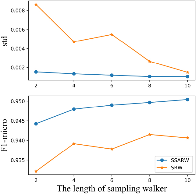

Figure 6.

The comparison between SSARW and SRW on PPI dataset.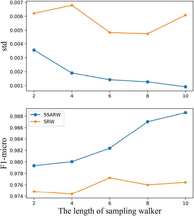

Figure 7.

The relationship between GCN depths and training time.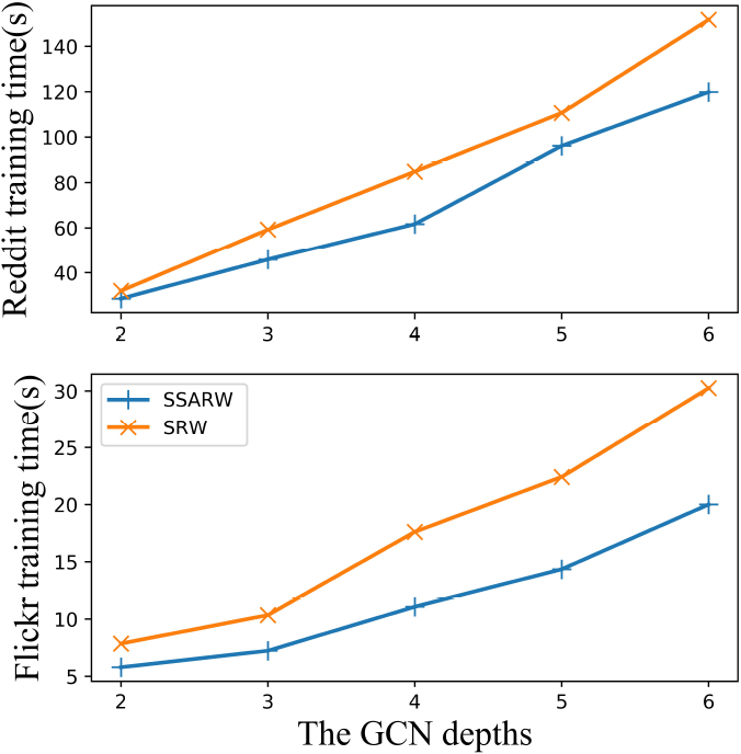

4.4 Addition discussion

In addition, we discuss some additional experiments. The training time of the SARW and SSARW methods are shorter. In Table 5, we compare the total training time and sampling time of our methods and the GraphSAINT-SARW approach. The GCN depth and the number of root nodes are the same in Table 2. The length of the walker is set as 10. We find the sampling time of the SARW and SSARW methods are both slightly higher than SRW, which may be because our sample method requires some judgment statements and calculations. However, the sampling time of our method is still a small order of magnitude, and the sampled subgraphs can be sampled in advance without taking up training time. From Table 5, the training time of the SARW and SSARW methods are less than that of the GraphSAINT-SRW method, which shows the superiority of our method. Moreover, the training time of the SARW is shorter than the SSARW, indicating that it is useful for SARW to consider the additional information of similar nodes. The sampling time of the SARW is longer than the SSARW, which shows the computation of the SARW is more complex.

In Fig. 7, we evaluate the training efficiency for different depths of GCN. We compare SSARW with GraphSAINT-SRW training on the two large graphs (Reddit and Flickr). We increase the number of layers and measure the average time per training execution. The GCN depth is set to 2, 3, 4, 5 and 6. Other settings are the same in Table 5. From Fig. 7, the total training time of GraphSAINT-SSARW and GraphSAINT-SRW are both roughly linear relationships with the GCN depth. This alleviates the “neighbor explosion” phenomenon (i.e., when increasing the depth, the training cost of GCN increases exponentially). Moreover, the training time of our method is less than that of the GraphSAINT-SRW method on both two datasets.

5. Conclusion

In this paper, we propose a new subgraph sampling method, SARW, which uses the edges, features and degree information to determine sampling probabilities. Our similarity-aware random walk subgraph sampling method achieves competitive performance for GCN training on large-scale graph data. Furthermore, we implement a simplified version of SARW called SSARW, which does not consider node features. We conduct a detailed theoretical analysis of SSARW, including unbiased learning of SSARW-based subgraph GCNs and a variance analysis. Extensive experiments on public datasets demonstrate the effectiveness of our proposed approach. Additionally, we study the influence of the sampling walker length, the relationship between GCN depths and training time. We also compare the sampling time between our method and the GraphSAINT-SRW method.

Our method addresses the problem of subgraph sampling on large-scale isomorphic and static graph data, but it is not suitable for non-isomorphic and dynamic graphs. In the future, we plan to extend our method to non-isomorphic and streaming graph data. Additionally, we aim to improve the manual sampling parameters to automatic parameters.

Footnotes

Acknowledgments

This work is supported by the National Natural Science Foundation of China under Grant (No. 62172372), the Natural Science Foundation of Zhejiang Province, China (No. LQ22F020033, No. LZ21F030001), and the Exploratory Research Project of Zhejiang Lab (No. 2022KG0AN01).

References

Zhou

Zheng

Huang

Hao

and Zhao

, Graph neural networks: Taxonomy, advances, and trends, ACM Trans. Intell. Syst. Technol. 13(1) (2022).

Kim

and Alice Oh KAIST

R.o.K.

, How to Find Your Friendly Neighborhood: Graph Attention Design with Self-supervision, in: ICLR, 2021.

Jiao

Chen

Liu

Yang

You

Liu

and Hou

, Graph Representation Learning Meets Computer Vision: A Survey, IEEE Transactions on Artificial Intelligence, 2022, 1–22.

Zhou

Cui

Zhang

Yang

Liu

Wang

and Sun

, Graph neural networks: A review of methods and applications, AI Open, 2020, 57–81.

Pan

Chen

Long

Zhang

and Yu

, A Comprehensive Survey on Graph Neural Networks, IEEE Transactions on Neural Networks and Learning Systems, 2020, 1–21.

Zhang

Cui

and Zhu

, Deep Learning on Graphs: A Survey, IEEE Transactions on Knowledge and Data Engineering, 2020.

Liang

Gui

Cambria

and Xu

, Aspect-based sentiment analysis via affective knowledge enhanced graph convolutional networks, Knowledge-Based Systems 235 (2022), 107643.

Gan

Kang

Peng

Zhu

and Zhu

, Multigraph Fusion for Dynamic Graph Convolutional Network, IEEE Transactions on Neural Networks and Learning Systems, 2022, 1–12.

Wang

Wei

Kuang

and Ding

, Graph Neural Networks with Node-Wise Architecture, in: KDD, Association for Computing Machinery, 2022, pp. 1949–1958.

10.

Souza

Zhang

Fifty

and Weinberger

, Simplifying Graph Convolutional Networks, in: ICML, 2019, pp. 6861–6871.

11.

Park

and Neville

, Exploiting Interaction Links for Node Classification with Deep Graph Neural Networks, in: IJCAI, 2019, pp. 3223–3230.

12.

Kipf

T.N.

and Welling

, Semi-Supervised Classification with Graph Convolutional Networks, in: ICLR, 2017.

13.

Bai

Lin

Miao

Liu

and Xu

, Efficient Data Loader for Fast Sampling-Based GNN Training on Large Graphs, IEEE Transactions on Parallel and Distributed Systems 32(10) (2021), 2541–2556.

14.

Zhao

Jiang

Chen

Qin

Xie

Liu

Zhou

Xia

and Zhou

, Preserving minority structures in graph sampling, IEEE Trans. Vis. Comput. Graph. 27(2) (2021), 1698–1708.

15.

Zhong

and Ye

, Efficient complementary graph convolutional network without negative sampling for item recommendation, Knowledge-Based Systems, 2022, 109758.

16.

Chen

Zhu

and Song

, Stochastic Training of Graph Convolutional Networks with Variance Reduction, in: ICML, Vol. 80, 2018, pp. 942–950.

17.

Zou

Wang

Jiang

Sun

and Gu

, Layer-Dependent Importance Sampling for Training Deep and Large Graph Convolutional Networks, in: NIPS, 2019.

18.

Chiang

Liu

Bengio

and Hsieh

, Cluster-GCN: An Efficient Algorithm for Training Deep and Large Graph Convolutional Networks, in: KDD, 2019.

19.

Bai

Ren

and Zhang

, Ripple Walk Training: A Subgraph-based Training Framework for Large and Deep Graph Neural Network, 2021, 1–8.

20.

Zeng

Zhou

Srivastava

Kannan

and Prasanna

, GraphSAINT: Graph sampling based inductive learning method, in: ICLR, 2020.

21.

Zeng

Zhang

Xia

Srivastava

Malevich

Kannan

Prasanna

Jin

and Chen

, Deep graph neural networks with shallow subgraph samplers, arXiv preprint arXiv:2012.01380, 2020.

22.

Yang

Liu

Dou

and Yu

P.S.

, ConsisRec: Enhancing GNN for Social Recommendation via Consistent Neighbor Aggregation, in: SIGIR, Association for Computing Machinery, 2021, pp. 2141–2145.

23.

Monti

Frasca

Eynard

Mannion

and Bronstein

M.M.

, Fake News Detection on Social Media using Geometric Deep Learning, arXiv preprint arXiv:1902.06673, 2019.

24.

Pal

Eksombatchai

Zhou

Zhao

Rosenberg

and Leskovec

, PinnerSage: Multi-Modal User Embedding Framework for Recommendations at Pinterest, in: KDD, 2020, pp. 2311–2320.

25.

Gao

Wang

and Li

, Graph Neural Networks for Recommender System, in: WSDM, 2022, pp. 1623–1625.

26.

Liu

You

Zhang

and Lv

, Tensor Graph Convolutional Networks for Text Classification, in: AAAI, 2020, pp. 8409–8416.

27.

Zhao

Hou

and Wu

, Modeling sentiment dependencies with graph convolutional networks for aspect-level sentiment classification, Knowledge-Based Systems 193 (2020), 105443.

28.

Nikolentzos

and Vazirgiannis

, Random Walk Graph Neural Networks, in: NeurIPS, 2020, pp. 16211–16222.

29.

Pei

Wei

Chang

K.C.-C.

Lei

and Yang

, Geom-GCN: Geometric Graph Convolutional Networks, in: ICLR, 2020.

30.

Zhang

Niu

Cui

Zhang

Cui

and Zhu

, A Simple and General Graph Neural Network with Stochastic Message Passing, arXiv preprint arXiv:2009.02562, 2020.

31.

Jiang

, Graph-based deep learning for communication networks: A survey, Computer Communications 185 (2022), 40–54.

32.

Chen

and Bruna

, Supervised Community Detection with Line Graph Neural Networks, in: ICLR, 2020.

33.

Abadal

Jain

Guirado

López-Alonso

and Alarcón

, Computing graph neural networks: A survey from algorithms to accelerators, ACM Computing Surveys (CSUR) 54(9) (2021), 1–38.

34.

Leskovec

and Jegelka

, How Powerful are Graph Neural Networks, in: ICLR, 2019.

35.

Bruna

Zaremba

Szlam

and LeCun

, Spectral networks and deep locally connected networks on graphs, in: ICLR, 2014.

36.

Hou

Huang

Wang

and Zhou

, Selective Attention Based Graph Convolutional Networks for Aspect-Level Sentiment Classification, in: Proceedings of the Fifteenth Workshop on Graph-Based Methods for Natural Language Processing (TextGraphs-15), 2021, pp. 83–93.

37.

Wang

Cao

Liu

and Chua

T.-S.

, KGAT: Knowledge Graph Attention Network for Recommendation, in: KDD, 2019, pp. 950–958.

38.

Hasanzadeh

Hajiramezanali

Boluki

Zhou

Duffield

Narayanan

and Qian

, Bayesian graph neural networks with adaptive connection sampling, in: International Conference on Machine Learning, PMLR, 2020, pp. 4094–4104.

39.

Cong

Forsati

Kandemir

and Mahdavi

, Minimal Variance Sampling with Provable Guarantees for Fast Training of Graph Neural Networks, in: KDD, 2020, pp. 1393–1403.

40.

Ying

Chen

Eksombatchai

Hamilton

W.L.

and Leskovec

, Graph Convolutional Neural Networks for Web-Scale Recommender Systems, in: KDD, 2018, pp. 974–983.

41.

Huang

Zhang

Rong

and Huang

, Adaptive Sampling towards Fast Graph Representation Learning, in: NIPS, 2018, pp. 4563–4572.

42.

Hamilton

W.L.

Ying

and Leskovec

, Inductive Representation Learning on Large Graphs, in: NIPS, 2017, pp. 1025–1035.

43.

Chen

and Xiao

, FastGCN: Fast Learning with Graph Convolutional Networks via Importance Sampling, in: ICLR, 2018.

44.

Zeng

Zhou

Srivastava

Kannan

and Prasanna

, Accurate, efficient and scalable graph embedding, in: 2019 IEEE International Parallel and Distributed Processing Symposium (IPDPS), IEEE, 2019, pp. 462–471.

45.

Wang

Cui

Wang

Pei

Zhu

and Yang

, Community Preserving Network Embedding, in: AAAI, 2017, pp. 203–209.

46.

Wei

Cao

and Yu

P.S.

, Embedding Identity and Interest for Social Networks, in: WWW, 2017, pp. 859–860.

47.

Lin

Xie

and Lui

J.C.s.

, Walking with Perception: Efficient Random Walk Sampling via Common Neighbor Awareness, in: ICDE, 2019, pp. 962–973.

48.

Lee

C.-H.

and Eun

D.Y.

, Beyond Random Walk and Metropolis-Hastings Samplers: Why You Should Not Backtrack for Unbiased Graph Sampling, in: SIGMETRICS, 2012, pp. 319–330.

49.

R.-H.

J.X.

Qin

Mao

and Jin

, On random walk based graph sampling, in: ICDE, 2015, pp. 927–938.

50.

Lovász

and Erdos

, Random walks on graphs: A survey, Combinatorics 2 (1993).

SARW: Similarity-Aware Random Walk for GCN

Abstract

Keywords

1. Introduction

1 https://github.com/houlinlinvictoria/SARW.

3. Methodology

3.1 SARW

.

Proof..

.

Proof..

.

Proof..

4.1 Data and settings

3 https://www.tensorflow.org/.

Table 4 The comparison between our SSARW and SRW on six datasets

5. Conclusion

Footnotes

Acknowledgments

References

¹
https://github.com/houlinlinvictoria/SARW.

³
https://www.tensorflow.org/.

Table 4
The comparison between our SSARW and SRW on six datasets