HSNF: Hybrid sampling with two-step noise filtering for imbalanced data classification

Abstract

Imbalanced data classification has received much attention in machine learning, and many oversampling methods exist to solve this problem. However, these methods may suffer from insufficient noise filtering, overlap between synthetic and original samples, etc., resulting in degradation of classification performance. To this end, we propose a hybrid sampling with two-step noise filtering (HSNF) method in this paper, which consists of three modules. In the first module, HSNF denoises twice according to different noise discrimination mechanisms. Note that denoising mechanism is essentially based on the Euclidean distance between samples. Then in the second module, the minority class samples are divided into two categories, boundary samples and safe samples, respectively, and a portion of the boundary majority class samples are removed. In the third module, different oversampling methods are used to synthesize instances for boundary minority class samples and safe minority class samples. Experimental results on synthetic data and benchmark datasets demonstrate the effectiveness of HSNF in comparison with several popular methods. The code of HSNF will be released.

Keywords

Imbalanced data classification oversampling noise fliter instance synthesis hybrid sampling

1. Introduction

Imbalanced data classification problem arises frequently in supervised learning and has received considerable attention from researchers in recent years. In other words, imbalanced data is also class imbalance. Generally, class imbalance can be divided into binary and multi-class imbalance, in terms of binary class imbalance that the most of the sample size belongs to the majority category, only a small portion belongs to the minority category [1]. The imbalance ratio (IR) can be used to express the degree of imbalance in datasets, which is defined as the ratio of the majority class to the minority class, a larger (smaller) IR indicates a higher (lower) degree of sample imbalance. At present, the class imbalance problem often occurs in many practical applications, such as fraud detection [2], disease diagnosis [3, 4], network intrusion detection [5, 6], detection of oil spills in radar images [7], environment resource management [8], and security management [9], etc. The final goal of classifiers is to achieve higher classification accuracy. However, traditional classification algorithms may not be used in class imbalance scenarios [10]. They may be affected by skewed distribution of data and cannot effectively identify minority class samples [11], even in cases of extreme imbalance, where minority samples cannot be identified. Therefore, the traditional classifier has a disadvantage in dealing with the class imbalance problem, that is, if all samples are identified as the majority class samples, the classification accuracy obtained may be very high, but this classification accuracy is worthless, because it is almost impossible to correctly identify the minority samples, and often important information is stored in the minority samples. For example, in the case of tumor cell detection, there is a class imbalance in this data. The number of majority class (representing normal, 90% of the dataset) in the dataset will be much more than the number of minority class (representing sick, 10% of the dataset), and if these data are directly taken to the traditional classifier for training, the classification accuracy will be as high as 90% if the classifier classifies all samples as normal, which means that the diseased samples will be misclassified as normal, and the cost of this misclassification is very huge. Class imbalance not only diminishes the performance of traditional classifiers, but also has an impact on deep learning. Ghosh et al. detailed the impact of class imbalance on deep learning architecture, such as the gradient of majority class is much larger than minority class, thus the majority class dominates the weight update of the model, and introduced the solution and future research direction [12].

Many methods have been proposed to deal with class imbalance. These methods can be classified into three categories: data-level methods [13, 14], cost-sensitive learning [15, 16], and ensemble learning [17, 18, 19]. Data-level methods use oversampling or undersampling to rebalance the data distribution. Cost-sensitive learning invokes the concept of cost matrix and assigns a larger cost to misclassified samples. Ensemble learning trains multiple subclassifiers and the final result is obtained from the voting results of each subclassifier.

Data-level methods mainly include oversampling and undersampling. Random oversampling [20, 21] and random undersampling [22] are the simplest oversampling and undersampling algorithms. The former is random replication of minority class instances from the dataset, while the latter is a random removal of majority class instances from the dataset, both to achieve a balanced distribution of data. For random oversampling, the model may be overfitted due to the random addition of minority class instances in the dataset, while random undersampling randomly removes most class samples from the dataset, which may contain important information and thus limit the performance of the classifier. Although both oversampling and undersampling exhibit their respective advantages and disadvantages, it has been demonstrated that the oversampling method is superior to the undersampling method in practical applications [23, 24]. Therefore, in this paper, we mainly discuss the oversampling method.

At present, many oversampling algorithms have been published in in the literature, including synthetic minority oversampling technique (SMOTE) [25], which is one of the most popular ones. Although SMOTE has shown excellent performance in dealing with class imbalance, it often ignores the distribution characteristics of minority and majority data and has a high probability of generating noisy samples, weakening the performance of the classifier. In order to solve the shortcomings of SMOTE, many SMOTE-based variant algorithms have been proposed, such as Borderline1-SMOTE [26], Borderline2-SMOTE [26], Safe-Level-SMOTE [27], ADASYN [28], ASN-SMOTE [29], etc. These SMOTE-based variant algorithms largely overcome the drawbacks of SMOTE, but introduce some new problems, such as small disjuncts problems [30], decision boundary overlap [31], and incomplete noise removal. In this paper, we propose a method hybrid sampling with two-step noise filtering for handling class imbalance in classification scenarios, this method can adequately filter noisy samples, reduce the overlap between synthetic samples and original samples, and improve the classification accuracy in the presence of class imbalance.

The main contributions of the paper are as follows:

•
We use different noise filtering mechanisms to conduct noise filtering twice to make the noise samples in the dataset more sufficiently filtered.
•
We divide the minority samples into safe minority samples and boundary minority samples and remove few boundary majority samples. The boundary minority samples are extremely imbalanced with respect to the majority samples, so we use the swim-rbf method to generate samples for them; the safe minority samples use adaptive qualified neighbor selection method to synthesize samples for them. The purpose is to reduce the overlap between the synthesized samples and the original samples.
•
We conduct extensive experiments show that the effectiveness of the proposed method compare to several popular methods by qualitative analysis and quantitative analysis.

The remainder of this article is organized as follows. We review some of the already existing oversampling methods in Section 2. In Section 3, we describe the proposed algorithm in detail. Experimental results and analysis are provided in Section 4. Finally,we we conclude this paper in Section 5.
2. Related work

The main purpose of oversampling is to increase the number of minority classes in an imbalanced dataset to make the dataset as balanced as possible. In this section, we briefly review some of the popular oversampling methods and their limitations.

Figure 1.

Random linear interpolation by using SMOTE (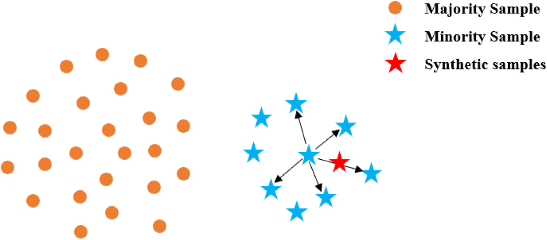 $K=5$ ).

Synthetic Minority Oversampling Technique (SMOTE) [25] is the most classical and widely used oversampling algorithm, which overcomes the problem of random oversampling that tends to produce overfitting. It generates synthetic minority samples by randomly interpolating between a minority class and its nearest minority classes. As shown in Fig. 1, Specifically, for a chosen minority class instance $x$ , first find the nearest $k$ minority class neighbors of $x$ , next choose a random instance $y$ from the $k$ minority class neighbors, and finally a new synthetic instance $z$ is randomly interpolated between the two chosen minority class instances by the Eq. (1):

$\displaystyle z=x+\alpha\times(y-x)$ (1)

where $\alpha$ is a random number ranging between [0, 1]. Although SMOTE has shown outstanding performance, it generates noisy instances that affect recognition accuracy, as shown in Fig. 2, because the algorithm randomly selects the nearest neighbors for sample synthesis, then it is possible to select minority instances located in the majority class region for synthesis, which generates noisy samples [31] and affects Classification performance.

Figure 2.

An example of possible noise generation when using SMOTE.

To overcome the above drawbacks, many improved algorithms of SMOTE have been proposed, such as Borderline-SMOTE [26], which instead of synthesizing all minority class instances, it introduces the number of majority classes $m$ in the $k$ nearest neighbors of a certain minority class and divides the minority class samples into three classes Safe, Danger, Noise respectively. Specifically, for a certain minority class sample, the minority class is classified as a Safe sample when $0\leqslant m<k/2$ , as a Danger sample when $k/2\leqslant m<k$ , and as a Noise sample when $m=k$ . Borderline-SMOTE oversamples only the minority class samples in Danger, and it is divided into Borderline1-SMOTE (B1-SMOTE) and Borderline2-SMOTE (B2-SMOTE) versions. The former only randomly selects instances among the $k$ nearest minority samples for sample synthesis, while the latter adds an option to select a nearest majority class sample for sample synthesis. However, the disadvantage of this method is that it may misclassify the borderline minority class samples as safe. Because of the sample distribution, all $k$ nearest neighbors of some borderline minority class instances are minority class, thus affecting the number of minority class instances on the decision boundary.

Safe-Level-SMOTE (SL-SMOTE) [27] introduces Safe-Level-Ratio, divides minority class samples into five cases according to Safe-Level-Ratio, and adjusts the position of synthetic instances for each case in order to make it closer to minority class sample. However, most of the sample positions generated by SL-SMOTE will be concentrated in the places where the minority class density is relatively concentrated, which avoids the generation of noisy instances but does not improve the recognition rate of minority classes on the decision boundary.

ADASYN [28] generates a different number of synthetic instances based on the size of the weight of each minority class. That is, the algorithm assigns different sampling weights to each minority class sample based on the number of majority class instances in the $k$ nearest neighbors of the minority class instances. During the sample synthesis phase, if the weight of that minority class instance is larger, then more synthetic instances are generated, and vice versa. However, ADASYN ignores the effect of noise, and for a noise instance whose $k$ nearest neighbors are all majority class, then it means assigning a large weight to that noise and finally generating more noise, which affects the classification accuracy.

K-means and SMOTE (KM-SMOTE) [32] is a combination of K-means clustering algorithm and SMOTE, which first clusters the input data samples using K-means algorithm, then calculates the imbalance ratio of each class cluster, filters according to the imbalance ratio, calculates the sampling weights, etc. It focuses on synthesizing instances only in safe regions especially safe sparse regions, so that although it avoids generating noisy instances and solving the within-class imbalance problem, however, finding a suitable number of clusters k is very difficult.

MWMOTE [31] redefines hard-to-learn samples by introducing $k_{1}$ , the number of nearest neighbors for each minority class sample (these nearest neighbors can be majority class, minority class or both) in order to filter noise; $k_{2}$ , the number of nearest neighbors for each minority class sample after removing noise (these nearest neighbors can only be majority class samples) in order to obtain the boundary majority class samples; $k_{3}$ , the number of nearest neighbors for each boundary majority class sample (these nearest neighbors can only be minority class samples) in order to obtain the hard-to-learn minority class samples. MWMOTE oversampling reduces the generation of noisy samples and improves the mechanism to discriminate the boundary samples, however, it ignores the minority clusters far from the majority class, even though these minority samples contain important information.

ASN-SMOTE [29] first filters noisy samples base on the Euclidean distance between samples. Then the minority class samples with the noise removed are combined with the whole data set to select qualified instances for linear interpolation. In particular, unlike the oversampling method mentioned above that brings the number of minority class samples to the same level as the number of majority class samples after processing is completed, this algorithm calculates the number of generated samples based on the number of samples in the dataset. ASN-SMOTE effectively avoids the effect of noisy samples and results in a more uniform distribution of synthetic samples. However, ASN-SMOTE has the problem of inadequate noise filtering. As show in Fig. 3, both minority class A and B should be considered as noise, but only B can be filtered out if noise filtering is performed with this algorithm.

Figure 3.

An example of inadequate noise filtering.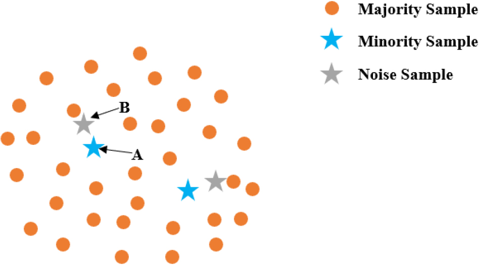

3. Method

In this section, we propose a new method that combines hybrid sampling and two-step noise filtering. The method not only effectively removes the noisy samples, but also greatly reduces the overlap between the synthetic samples and the original boundary samples, which makes the classification decision boundary more reasonable and improves the recognition accuracy of minority samples and the classification performance. The flowchart of the HSNF approach is shown in Fig. 4, which mainly consists of noise filtering and dividing the minority class samples into two categories and then processing them by different methods.

Figure 4.

The flowchart of HSNF method.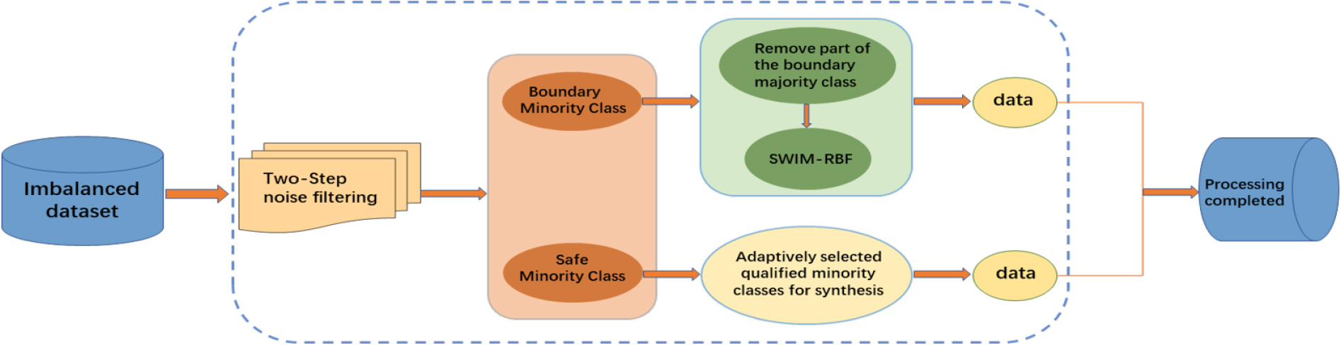

3.1 Preliminary

Before introducing the proposed method in detail, we introduce the SWIM-RBF algorithm. SWIM-RBF is an effective method for dealing with extreme imbalances by using the density distribution of minority class samples relative to majority class samples in a dataset to guide the generation of samples, rather than using Euclidean distances between samples. SWIM-RBF uses a radial basis function with a Gaussian kernel to evaluate the density of the minority class relative to the majority class, and the Gaussian kernel is computed by the Eq. (2):

$\displaystyle H(r)=\exp-(ur)^{2}$ (2)

where $u$ and $r$ are the smoothing and distance parameters, respectively. In general, $u$ is a value close to zero because a smaller value of $u$ makes the function smoother and more generalizable. We divide the dataset into two subsets as the majority class set Maj and the minority class set Min, as show in Fig. 5, We first calculate the score for each minority class sample, and the calculation is based on the density of that minority class relative to the majority class sample, which yields a different score. The density of the areas represented by A, B, and C in the figure increases in order, $n\in\textit{Min}$ , $m\in\textit{Maj}$ , Scores are calculated by the Eq. (3):

$\displaystyle\textit{rbf\_score}(n)=\sum_{i=1}^{|\textit{Maj}|}H(||m_{i}-n||)_% {2}$ (3)

in the instance generation phase, regions with the same or lower density than the current minority class are selected for sample synthesis based on the size of rbf_score.

Figure 5.

Generate instances using the density of the minority class relative to the majority class distribution.

[h] : Two-step noise filtering[1] Input Data(Q), Dividing the dataset into majority(Maj) and minority classes(Min) for $i$ in 1, …, $\textit{len}(\textit{Min})$ do $D(a_{\min}^{i})=\mathop{\arg\min}\limits_{a_{i}\in\textit{Min},q\in Q,q\neq a_% {i}}||a_{i}-q||_{2}$ if $D(a_{\min}^{i})\in\textit{Maj}$ then $\textit{Min\_filter}=\textit{Min\_filter}\cup a_{i}$ else $\textit{Min}_{1}=\textit{Min}_{1}\cup a_{i}$ end if end forAfter the first noise filtering is completed, we get the minority class set $\textit{Min}_{1}$ , the whole data set $\textit{Q\_filter}:\textit{Q-Min\_filter}$ for each $b_{i}\in\textit{Min}_{1},i=1,\ldots,\textit{len}(\textit{Min}_{1})$ do Find the $K$ nearest neighbors of $b_{i}$ in Q_filter, and denote by $m$ the number of nearest neighbors belonging to the majority class if $K/2\leqslant m<K$ then $\textit{Min}_{1}\_\textit{border.append}(b_{i})$ else if $m=k$ then $\textit{Min}_{1}\_\textit{noise.append}(b_{i})$ end else if end if $\textit{Min}_{1}\_\textit{safe}=\textit{Min}_{1}-\textit{Min}_{1}\_\textit{% noise}-\textit{Min}_{1}\_\textit{border}$ end for

3.2 HSNF method

We combine ASN-SMOTE, Borderline-SMOTE, Undersampling and SWIM-RBF methods to divide the minority samples into different categories, and to reduce the chance of overlap between the synthetic samples and the original samples, especially the boundary majority class samples, we remove some of the boundary majority class samples and use different methods to synthesize samples for different categories. specifically, our approach can be divided into three steps.

3.2.1 Step 1: Two-step noise filtering

As show in Algorithm 5, we divide the input data set(denoted by Q) into majority class set (denoted by Maj), and minority class set (denoted by Min). First, for each $a_{i}\in\textit{Min}$ , find the nearest neighbor to itself and stored in $D(a_{\min}^{i})$ . If $D(a_{\min}^{i})\in\textit{Maj}$ , $a_{i}$ is treated as noise. After the first denoising step, we get minority class set (denoted by $\textit{Min}_{1}$ ), the overall dataset (denoted by Q_filter). Then, for each $b_{i}\in\textit{Min}_{1}$ , find the $k$ nearest neighbors of $b_{i}$ in Q_filter, denote by $m$ the number of the $k$ neighbors belonging to the majority class. If $k/2\leqslant m<k$ , then $b_{i}$ is the boundary minority class and stored with $\textit{Min}_{1}\_\textit{border}$ , if $m=k$ , then $b_{i}$ is the minority class noise and stored in $\textit{Min}_{1}\_\textit{noise}$ , Final, the safe minority class sample $\textit{Min}_{1}\_\textit{safe}=\textit{Min}_{1}-\textit{Min}_{1}\_\textit{% border}-\textit{Min}_{1}\_\textit{noise}$ . After the above steps are completed, we are done with noise filtering for two times. This method can filter the noise more fully. As shown in Fig. 5, after the first step of noise filtering, only noise A is filtered out, while noise B remains in the majority class, and after the second step of noise filtering is completed, noise B is also filtered.

[h] : Remove some boundary majority classes and use SWIM-RBF for boundary minority classes[1] Input data set $\textit{Min}_{1}\_\textit{border}$ , Maj, $P_{1}=\textit{Min}_{1}\_\textit{border}+\textit{Maj}$ $i$ in 1, …, $\textit{len}(\textit{Maj})$ $d(g_{\min}^{i})=\mathop{\arg\min}\limits_{{g_{i}\in\textit{Maj},t\in P_{1},t% \neq g_{i}}}||g_{i}-t||_{2}$ $d(g_{\min}^{i})\in\textit{Min}_{1}\_\textit{border}$ $\textit{Maj\_border}=\textit{Maj\_border}\cup g_{i}$ $\textit{Maj}_{1}=\textit{Maj}-\textit{Maj\_border}$ SWIM-RBF algorithm is used: $\delta$ , standard deviation for Gaussian jitter; N_socre, estimated den- sity of the minority class instances; $\textit{Maj}_{1}$ , majority class instances; $\textit{Min}_{1}\_\textit{border}$ , minority class instances; S, a synthetic minority sample. repeat: $S=\textit{Min}_{1}\_\textit{border}+\lambda(0,\delta)$ $\textit{S\_score}=\textit{rbf\_score}_{\textit{Maj}_{1}}(S)$ until $\textit{S\_score}\leqslant\textit{N\_score}$ and $\textit{attempts}\leqslant\textit{maxAttempts}$ $\textit{attempts}\leqslant\textit{maxAttempts}$ $S=\textit{Min}_{1}\_\textit{border}$ return S

[b] : Oversampling of safe minority classes using ASN-SMOTE[1] Input data set $Q$ , $\textit{Min}_{1}\_\textit{safe}$ for each $w_{i}\in\textit{Min}_{1}\_\textit{safe},i=1,\ldots,\textit{len}(\textit{Min}_{% 1}\_\textit{safe})$ do Find the $K$ nearest neighbors in the data set $Q$ in the order of smallest to largest except $w_{i}$ itself for $m=1$ to $k$ do if $w_{i}^{m}\in\textit{Maj}$ then $Q_{1}=Q_{1}\cup w_{i}^{m}$ break else $Q_{1}=Q_{1}\cup w_{i}^{m}$ end if end for for $i=1$ to $n$ do $\textit{synthetic}=w_{i}+\alpha(q_{i}-w_{i})$ , $q_{i}\in Q_{1}$ end for end for

3.2.2 Remove some boundary majority classes and use SWIM-RBF for boundary minority classes

As show Algorithm 3.2.1, following the completion of the first step, we can obtain the boundary minority class $\textit{Min}_{1}\_\textit{border}$ , the majority class Maj, and the union set $P_{1}$ of the above two. For each $g_{i}\in\textit{Maj}$ , find the nearest neighbor to itself and stored in $d(g_{\min}^{i})$ . If $d(g_{\min}^{i})\in\textit{Min}_{1}\_\textit{border}$ , $g_{i}$ is treated as the boundary majority class closest to a certain boundary minority class and deleted. Next, the SWIM-RBF algorithm is used. For any minority class $\textit{Min}_{1}\_\textit{border}$ , first calculate its density fraction with respect to the majority class denoted by N_score. Then a synthetic instance $S$ is synthesized through the equation $S=\textit{Min}_{1}\_\textit{border}+\lambda(0,\delta)$ , where, $\delta$ is standard deviation for Gaussian jitter. Next, calculate the relative density fraction S_score of the synthetic example $S$ , repeat the above procedure until $\textit{S\_score}\leqslant\textit{N\_score}$ . As show Fig. 5, The purpose is to reduce the probability that the synthesized boundary minority class samples overlap with the boundary majority class samples. For a more detailed description, please refer to paper SWIM [33].

3.2.3 Oversampling of safe minority classes using ASN-SMOTE

As show Algorithm 3.2.1, for each $w_{i}\in\textit{Min}_{1}\_\textit{safe}$ , find the $K$ nearest neighbors in the data set $Q$ in the order of smallest to largest except $w_{i}$ itself. Use the set $Q_{1}$ to store the qualified neighbors, and judge the label of these $K$ nearest neighbors in sequence. If the label belongs to the minority class, the nearest neighbor is stored in $Q_{1}$ and continues to judge until the kth neighbor is judged, and if the label belongs to the majority class, the current nearest neighbor is stored in $Q_{1}$ and exits the current loop. Then, a nearest neighbor is randomly selected from $Q_{1}$ . The synthetic instance is performed using the equation in line 12 of Algorithm 3 and the synthesis process is executed $n$ times, where, $n=\frac{\textit{Maj}-\textit{Min}}{\textit{Min}_{1}}$ is the number of samples to be synthesized for each minority class of samples. The above is the process of safe minority class oversampling.

The pseudocode of the proposed method is described in Algorithms 5, 3.2.1, and 3.2.1. For Algorithms 1, 2, and 3, we have two remarks.

.

The two-step noise filtering is based on the Euclidean distance between samples. The first step of noise filtering uses the Euclidean distance between minority class samples and the whole datasets; the second step of noise filtering uses the Euclidean distance between the minority class samples and the whole datasets after removing the noise from the previous step.

.

When the second noise filtering step is finished, the division of minority class samples into safe minority class and boundary minority class is completed simultaneously.

4. Experiments

In this section, we perform experiments to verify the effectiveness of the proposed algorithm HSNF, and report the comparison results on both synthetic data and benchmark datasets.

4.1 Experimental settings

To test the performance of the proposed method, we used 16 benchmark imbalanced datasets and compared the proposed method with Random Oversampling (ROS), SMOTE [25], ADASYN [28], B1-SMOTE [26], B2-SMOTE [26], SL-SMOTE [27], D-SMOTE [34], KM-SMOTE [32], ASN-SMOTE [29], the data for comparison are obtained by running KNN [35], SVM [36], and GaussianNB (NB) classifiers. The oversampling methods and classifiers used in the experiments can be found in smote_variants [37], sklearn [38], and imbalanced-learn [39], respectively. Where, for the parameters of the SVM classifier, we set the penalty term to $L2$ , $C=0.1$ , $\textit{max\_iter}=10000$ , and loss to be the hinge loss, and the parameters of the other classifier and oversampling methods employed use default values. We use fivefold stratified cross validation to divide the training and test sets in order to reduce overfitting. Each experiment was performed three times to take the average in order to decrease the effect of randomness.

4.2 Benchmark dataset description

We conduct comparison experiments with 16 datasets that come from Keel1

¹
https://sci2s.ugr.es/keel/datasets.php##sub1.

and UCI,2

https://archive.ics.uci.edu/ml/index.php.

the characteristics of these datasets are shown in Table 1. As shown in this table, these datasets have different attributes, sample numbers and degrees of imbalance. There are datasets with labels of multiple classes, such as “Iris”, “Ecoli”, etc., which we need to convert to two classes. (Ecoli, Iris, Parkinsons)3

https://raw.githubusercontent.com/M-Hashemzadeh/RCSMOTE/master/ImplementationSourceCodes.zip.

and (Heart2, Liver_disorders2, Vehicle2)4

⁴

https://github.com/felix-last/evaluate-kmeans-smote/releases/download/v0.0.1/uci_extended.tar.gz.

datasets labels are converted into two-class versions can be found in the link annotated at the bottom of this page. Specifically, the experiments in this paper use label 0 to represent the minority class and label 1 to represent the majority class.

Table 1

Description of the datasets

Dataset	Attributes	Majority	Minority	Instances	IR
Yeast-0-5-6-7-9_vs_4	8	477	51	528	9.35
Ecoli	7	301	35	336	8.6
Wine	13	119	59	178	2.02
Haberman	3	225	81	306	2.78
Ecoli3	7	301	35	336	8.6
Ecoli1	7	259	77	336	3.36
Iris	4	100	50	150	2.00
Parkinsons	22	147	48	195	3.06
Yeast5	8	1440	44	1484	32.73
Yeast-0-2-5-6_vs_3-7-8-9	8	905	99	1004	9.14
Heart2	13	150	60	210	2.5
Liver_disorders2	6	200	72	272	2.78
Vehicle2	18	647	99	746	6.54
Glass0	9	144	70	214	2.06
Pima	8	500	268	768	1.87
Ecoli-0-1-4-7_vs_5-6	6	307	25	332	12.28

4.3 Evaluation metrics

We mentioned in introduction that the traditional evaluation metrics are no longer applicable to class imbalance scenarios. Therefore, we use F-measure, G-mean, and AUC as evaluation criteria [40], which are defined by Eqs (4)–(8), respectively. where, TP indicates the number of minority (positive) classes correctly classified, FP indicates the number of majority (negative) classes misclassified as minority (positive) classes, TN indicates the number of majority (negative) classes correctly classified, and FN indicates the number of minority (positive) classes misclassified as majority (negative) classes.

$\displaystyle\textit{F-measure}=\frac{2\times\textit{Sensitivity}\times\textit% {Precision}}{\textit{Sensitivity}+\textit{Precision}}$ (4) $\displaystyle\textit{G-mean}=\sqrt{\textit{Sensitivity}\times\textit{% Specificity}}$ (5) $\displaystyle\textit{AUC}=\frac{1+\textit{TPR}-\textit{FPR}}{2}$ (6)

Sensitivity: The probability of actual positive samples being predicted as positive samples; Precision: The probability of actual positive samples out of all the samples predicted to be positive; Specificity: The probability of actual negative samples being predicted as negative samples. These are defined as follows.

$\displaystyle\textit{Sensitivity}=\frac{TP}{TP+FN},\textit{Precision}=\frac{TP% }{TP+FP},\textit{Specificity}=\frac{TN}{TN+FP}$ (7) $\displaystyle\textit{TPR}=\frac{TP}{\textit{Minority class number}},\textit{% FPR}=\frac{FP}{\textit{Majority class number}}$ (8)

4.4 Result and discussion

4.4.1 Results visualization on two-dimensional synthetic data

The purpose of data visualization is to observe the data distribution after applying the oversampling method to the original data set. We create the circle and moon datasets using the make_circles and make_moons methods in sklearn, then the two datasets are processed by the HSNF method and the comparison method, respectively. As shown in Figs 6 and 7 respectively, we can see that the minority samples generated using HSNF are more uniformly distributed, more adequately filtered for noise, and less overlapping with the boundary samples than the comparison method.

Figure 6.

Distribution of circle data after using different sampling methods.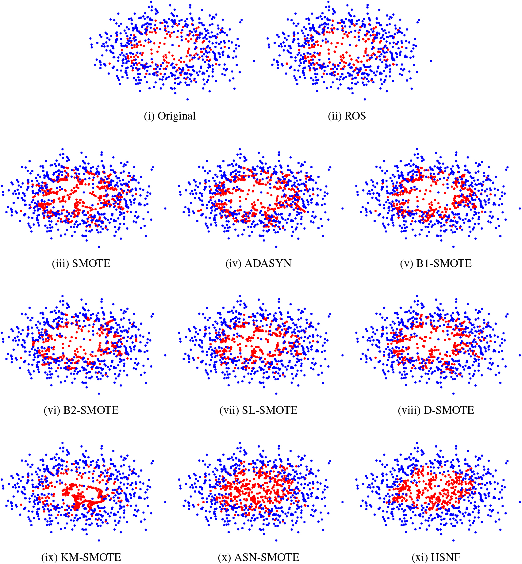

Figure 7.

Distribution of moon data after using different sampling methods.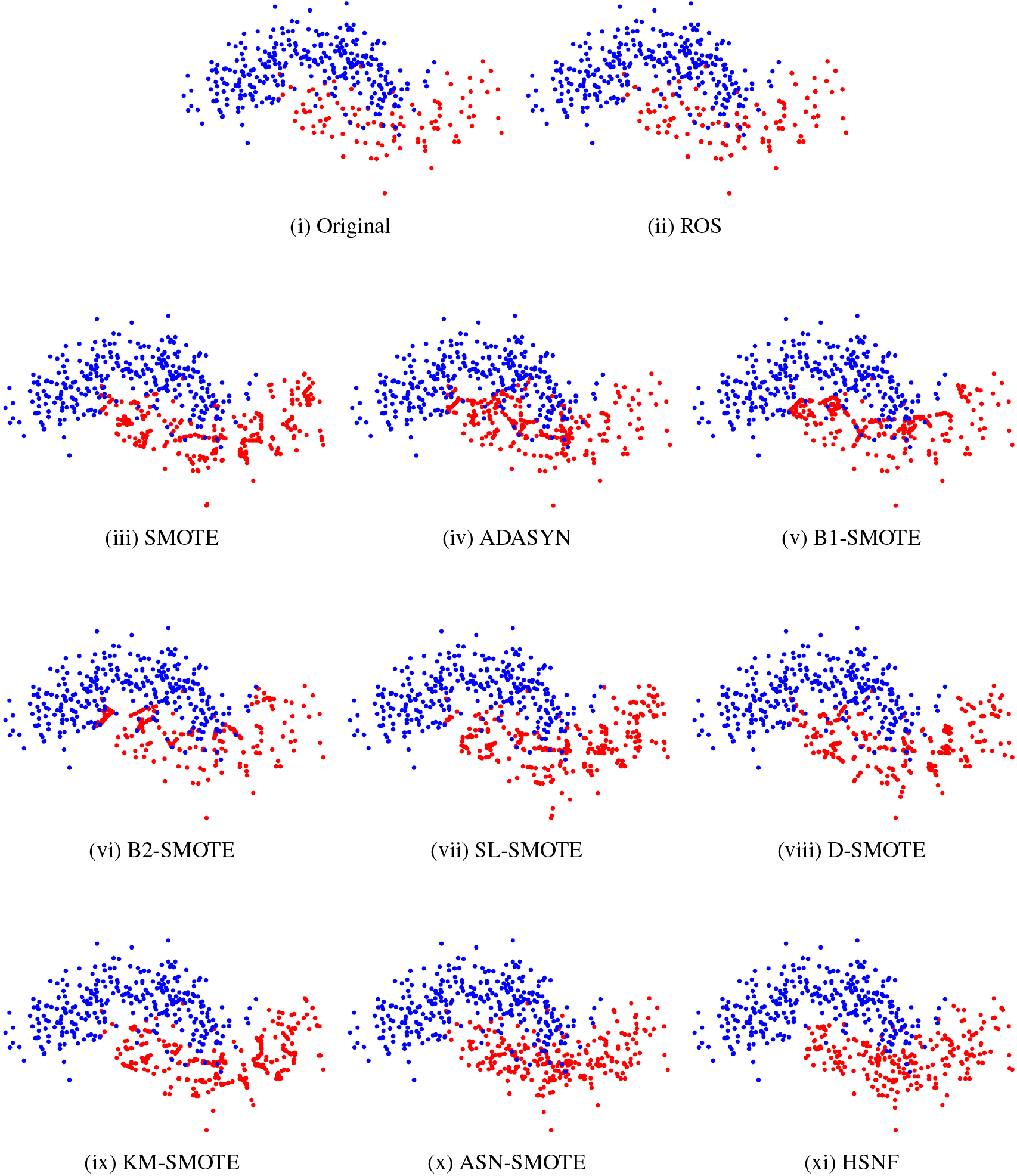

4.4.2 Quantitative comparison on experiment results

In this subsection, we evaluate the performance of the HSNF method on the benchmark dataset. Tables 3 to 10 show the experimental results of our method and the comparison method on KNN, NB, and SVM classifiers, respectively. As shown in tables, the best results are shown in red font and the second best results are shown in blue font. Figure 8 shows the average ranking of each method on the 16 benchmark datasets,specifically, smaller ranking averages represent higher performance. Wilcoxon signed rank test is used to test whether the difference between the proposed method and the comparison method is statistically significant. Results are shown in Table 11, $p$ values with statistically significant differences at the significance level of $\alpha=0.05$ are marked in bold.

Tables 3 to 5 show the results of using F-measure, G-mean, and AUC as evaluation metrics on the KNN classifier. As shown in Tables 3 to 5, the HSNF method obtains the highest number of sums of optimal and suboptimal values on F-measure and G-mean, and the sum of optimal and suboptimal values obtained by HSNF on AUC is comparable to ASN-SMOTE. But, HSNF has the highest ranking on three measures (Fig. 8), which indicates that our method outperforms the comparison method. From Table 11, it can be concluded that the HSNF method significantly outperforms ADASYN, B2-SMOTE, SL-SMOTE and ASN-SMOTE on F-measure, significantly outperforms KM-SMOTE on G-mean and significantly outperforms B1-SMOTE on AUC.

Tables 5 to 7 show the results of using F-measure, G-mean, and AUC as evaluation metrics on the NB classifier. As shown in Tables 5 to 7, the HSNF method obtains the highest number of sum of optimal and suboptimal values on AUC, and the sum of optimal and suboptimal values on F-measure and G-mean is competitive with KM-SMOTE and more than other comparison methods. In addition, the HSNF method obtains the highest ranking in all three measures (Fig. 8), and HSNF significantly outperforms B2-SMOTE and SL-SMOTE in F-measure and KM-SMOTE in G-mean (Table 11).

Tables 9 to 10 show the results of using F-measure, G-mean, and AUC as evaluation metrics on the SVM classifier. As shown in Tables 9 to 10, the HSNF method obtains the highest number of sum of optimal and suboptimal values on F-measure and AUC, and is ranked with ADASYN, B2-SMOTE and

Table 2
F-measure results obtained using KNN classifier on 16 datasets

Data	ROS	SMOTE	ADASYN	B1-SMOTE	B2-SMOTE	SL-SMOTE	D-SMOTE	KM-SMOTE	ASN-SMOTE	HSNF
Yeast-0-5-6-7-9_vs_4	red0.507636	0.48774	0.473483	0.456374	0.439081	0.457943	blue0.490704	0.446416	0.47121	0.451799
Ecoli	0.554689	0.54507	0.562411	0.573083	0.565195	0.562038	0.556216	blue0.594814	0.584649	red0.596853
Wine	0.844447	0.831657	blue0.856296	red0.87849	0.849069	0.831657	0.820418	0.833569	0.834418	0.842234
Haberman	0.420924	0.437401	0.417259	0.423661	0.4314	blue0.4522	0.430904	0.392326	0.422518	red0.457029
Ecoli3	0.590735	0.59593	0.587821	0.638349	0.584919	0.586488	0.582197	blue0.642647	0.605702	red0.671207
Ecoli1	0.767392	0.761983	0.716714	0.747474	0.746468	0.744305	0.757391	blue0.777178	0.735109	red0.789831
Iris	0.922334	0.922334	0.891609	0.915088	0.893696	0.90597	0.915419	blue0.935556	0.921668	red0.938897
Parkinsons	0.401167	blue0.415566	0.401865	nan	nan	nan	nan	nan	nan	red0.496354
Yest5	red0.669183	0.650928	0.645916	0.646617	0.580827	0.61756	blue0.662909	0.650595	0.595948	0.618592
Yeast-0-2-5-6_Vs_3-7-8-9	0.421908	0.405615	0.344864	0.423114	0.438455	0.425842	0.381501	0.500923	blue0.509439	red0.558125
Heart2	0.510725	0.528678	0.536963	0.5366	0.527769	0.533464	blue0.542891	0.498647	red0.551123	0.541522
Liver_disorders2	blue0.500932	0.476836	0.488726	0.498235	0.466282	0.495939	0.478016	0.375091	0.442101	red0.526954
Vehicle2	blue0.736717	0.721916	0.718465	0.735435	0.681988	0.719242	0.722596	red0.753948	0.646743	0.724202
Glass0	0.678641	0.689576	0.701141	0.687937	blue0.703132	0.684184	red0.722105	0.670242	0.666015	0.660743
Pima	0.586211	0.574454	0.5943	0.593503	blue0.594555	0.58939	0.593457	0.574793	red0.602979	0.574064
Ecoli-0-1-4-7_vs_5-6	0.704824	blue0.708915	0.665716	0.693142	0.70101	0.684183	0.688283	0.676487	0.627232	red0.736111

Table 3

G-mean results obtained using KNN classifier on 16 datasets

Data	ROS	SMOTE	ADASYN	B1-SMOTE	B2-SMOTE	SL-SMOTE	D-SMOTE	KM-SMOTE	ASN-SMOTE	HSNF
Yeast-0-5-6-7-9_vs_4	0.787121	red0.7995	blue0.797597	0.745862	0.752181	0.772385	0.796351	0.671145	0.766449	0.675096
Ecoli	0.843168	0.829955	0.844569	0.82358	0.834958	red0.856748	0.832783	0.804154	blue0.853335	0.830077
Wine	0.883716	0.875055	blue0.899608	red0.918304	0.891908	0.875055	0.866084	0.868324	0.875453	0.878567
Haberman	0.580703	0.597194	0.579827	0.581035	0.585995	blue0.605373	0.59007	0.541924	0.585147	red0.608308
Ecoli3	0.865415	0.867081	0.865651	blue0.8788	0.872799	0.874096	0.851844	0.868086	0.869143	red0.885668
Ecoli1	blue0.85573	0.85413	0.827396	0.838873	0.832924	0.841811	0.85192	0.849973	0.838937	red0.866711
Iris	0.942821	0.942821	0.921766	0.936993	0.91979	0.932817	0.938727	blue0.948027	0.943537	red0.953954
Parkinsons	0.548343	blue0.56606	0.554951	0.511668	0.478523	0.525748	0.491209	0.516602	0.552051	red0.62006
Yest5	0.950251	0.960793	blue0.960821	0.949453	0.944795	0.958396	red0.961858	0.88749	0.957029	0.9588
Yeast-0-2-5-6_Vs_3-7-8-9	0.719957	0.722025	0.692177	0.676029	0.684449	blue0.722393	0.697505	0.662605	0.706866	red0.724329
Heart2	0.644163	0.66045	0.665274	0.666903	0.659391	0.665286	blue0.672594	0.628359	red0.679105	0.671554
Liver_disorders2	red0.649873	0.628593	0.640739	0.646445	0.621972	blue0.648952	0.629062	0.522657	0.599808	0.644222
Vehicle2	0.910581	0.905695	0.908295	blue0.916805	0.90103	0.912702	0.905635	0.847707	0.894175	red0.921343
Glass0	0.752106	0.758845	0.765757	0.756775	blue0.768399	0.75076	red0.788997	0.746597	0.740768	0.741406
Pima	0.671145	0.661774	0.670804	0.671861	0.668403	0.673898	blue0.676008	0.664785	red0.688583	0.664945
Ecoli-0-1-4-7_vs_5-6	0.817604	red0.827255	0.808087	0.791268	0.823366	blue0.827059	0.810361	0.788435	0.771136	0.806439

Table 4

AUC results obtained using KNN classifier on 16 datasets

Data	ROS	SMOTE	ADASYN	B1-SMOTE	B2-SMOTE	SL-SMOTE	D-SMOTE	KM-SMOTE	ASN-SMOTE	HSNF
Yeast-0-5-6-7-9_vs_4	0.835261	red0.88543	0.874604	0.832388	0.865248	0.868244	0.869393	0.825066	blue0.874986	0.770476
Ecoli	0.881655	0.888365	0.90573	0.893048	0.908341	red0.917654	0.893977	0.887034	blue0.917631	0.900078
Wine	0.971838	0.967527	0.949793	0.95099	0.960616	0.961657	0.955803	red0.978627	blue0.971886	0.968809
Haberman	0.649289	0.647737	0.630686	0.642304	blue0.649608	0.636912	0.635319	0.640817	0.651528	red0.651528
Ecoli3	0.900835	0.903872	0.902955	0.911019	red0.921998	0.90888	0.902701	blue0.917186	0.904906	0.90929
Ecoli1	0.910476	0.914943	0.910135	0.90377	0.901937	0.91967	0.924185	0.924246	red0.932849	blue0.924841
Iris	0.989	0.9845	0.979237	0.983737	0.982237	blue0.9885	0.989	0.989	0.988	red0.989
Parkinsons	0.594506	0.592307	0.609333	0.574559	0.599414	0.623257	0.586782	0.624559	blue0.631908	red0.675153
Yest5	0.967385	0.966922	0.966035	0.967226	0.965133	0.966797	0.967467	0.969112	blue0.973973	red0.977739
Yeast-0-2-5-6_Vs_3-7-8-9	0.774721	0.765638	0.75694	0.758876	0.771058	blue0.78403	0.76081	red0.802232	0.782329	0.779842
Heart2	0.69	0.675278	0.675	0.700278	0.684722	0.707222	0.688889	0.7025	blue0.718611	red0.729722
Liver_disorders2	0.685048	0.672607	0.664512	0.681655	0.668524	blue0.693393	0.68656	0.667679	0.675036	red0.699357
Vehicle2	0.956635	blue0.969009	0.96892	red0.969756	0.951835	0.961534	0.956007	0.960129	0.954347	0.963344
Glass0	0.855621	0.858612	0.868482	0.870408	red0.88143	0.85811	0.873962	blue0.874411	0.859817	0.852155
Pima	0.72808	0.729726	0.729927	0.727284	0.730853	0.743416	0.74032	0.742657	blue0.751451	red0.757389
Ecoli-0-1-4-7_vs_5-6	0.835447	blue0.847583	red0.857462	0.812179	0.842041	0.832887	0.827277	0.836108	0.826653	0.824601

Table 5

F-measure results obtained using NB classifier on 16 datasets

Data	ROS	SMOTE	ADASYN	B1-SMOTE	B2-SMOTE	SL-SMOTE	D-SMOTE	KM-SMOTE	ASN-SMOTE	HSNF
Yeast-0-5-6-7-9_vs_4	0.172405	0.176587	0.178187	blue0.182163	0.1767	0.176358	0.179868	red0.229859	0.179713	0.177967
Ecoli	0.264977	0.388295	0.30791	blue0.408566	0.341667	0.306479	0.337703	red0.449048	0.398281	0.393403
Wine	0.931377	0.949767	0.959253	blue0.961111	0.953698	red0.966609	0.956456	0.945342	0.9509	0.946733
Haberman	0.43087	0.414133	0.427532	0.410381	red0.44381	0.40177	blue0.43468	0.379275	0.404635	0.425372
Ecoli3	0.441396	0.515326	0.444719	0.529856	0.53546	0.48873	0.5009	blue0.55486	0.518222	red0.576011
Ecoli1	0.545033	0.604756	0.563188	0.613521	0.615116	0.59986	0.611841	0.626435	red0.656575	blue0.634524
Iris	0.835673	0.820016	0.818109	0.80394	0.796342	0.822601	0.828398	blue0.84617	0.822601	red0.848895
Parkinsons	0.537229	0.539129	0.520149	0.535367	0.480186	0.496037	0.537134	blue0.546042	0.514505	red0.54987
Yest5	0.123703	0.189377	0.167939	0.172039	0.097425	0.167512	red0.232481	0.162302	blue0.198306	0.177694
Yeast-0-2-5-6_Vs_3-7-8-9	0.481247	0.493874	0.48683	0.41181	0.429538	0.488686	0.484243	0.191947	blue0.512162	red0.529163
Heart2	red0.774501	0.722442	blue0.764088	0.738971	0.743242	0.70866	0.735378	0.731768	0.758797	0.741485
Liver_disorders2	0.416162	0.406436	0.406677	blue0.419732	0.411296	0.405697	red0.423527	0.27754	0.38411	0.396058
Vehicle2	0.376462	red0.392014	0.361759	0.361712	0.348785	0.372919	blue0.385723	nan	0.371586	0.365414
Glass0	0.641323	blue0.654995	0.625476	0.61319	0.618784	0.644067	0.625476	red0.667063	0.637488	0.625843
Pima	blue0.6504	0.649887	0.643931	0.645465	0.639904	0.64454	0.639651	0.58983	red0.654738	0.647971
Ecoli-0-1-4-7_vs_5-6	0.67671	red0.719206	0.681111	0.650769	nan	blue0.689607	0.6825	nan	0.666405	nan

Table 6

G-mean results obtained using NB classifier on 16 datasets

Data	ROS	SMOTE	ADASYN	B1-SMOTE	B2-SMOTE	SL-SMOTE	D-SMOTE	KM-SMOTE	ASN-SMOTE	HSNF
Yeast-0-5-6-7-9_vs_4	0.131783	0.232432	0.227281	blue0.297051	0.242813	0.187911	0.269779	red0.502284	0.268577	0.152603
Ecoli	0.523265	0.711698	0.606987	0.75151	0.708214	0.575207	0.677221	blue0.751838	0.728722	red0.768794
Wine	0.947933	0.961513	0.970425	blue0.974537	0.970054	red0.974549	0.961513	0.947661	0.961142	0.956269
Haberman	0.560456	0.548795	0.563339	0.547371	red0.576396	0.539833	blue0.570486	0.509134	0.54986	0.55662
Ecoli3	0.800715	0.864046	0.801139	0.852945	0.862196	0.840585	0.839986	blue0.869583	0.842804	red0.872144
Ecoli1	0.667204	0.743565	0.697733	0.747203	0.728831	0.734733	0.752339	blue0.760512	red0.803779	0.758551
Iris	0.869832	0.856841	0.850638	0.836705	0.817571	0.858279	0.863864	blue0.879633	0.858279	red0.879972
Parkinsons	0.694885	0.696051	0.673269	0.691767	0.610298	0.647541	0.694269	blue0.6966	0.663968	red0.700704
Yest5	0.751056	0.849672	0.82194	0.82176	0.629512	0.829522	red0.88126	0.822712	blue0.853152	0.834055
Yeast-0-2-5-6_Vs_3-7-8-9	0.558014	0.565505	0.611612	0.581894	0.612535	0.567679	0.563745	0.339777	blue0.630204	red0.643484
Heart2	red0.852482	0.809922	blue0.843022	0.822766	0.838867	0.810168	0.808865	0.797815	0.839654	0.820228
Liver_disorders2	0.43389	0.445507	0.446631	0.443617	0.45973	0.442986	blue0.488953	0.389816	0.440618	red0.549186
Vehicle2	0.707002	red0.724557	0.68944	0.688531	0.673712	0.702289	blue0.717765	0.28381	0.701211	0.693815
Glass0	0.623064	blue0.653284	0.623179	0.607876	0.602568	0.639171	0.623179	red0.664414	0.636931	0.622256
Pima	blue0.727181	0.727062	0.721934	0.723853	0.718003	0.722589	0.718948	0.673674	red0.73003	0.723792
Ecoli-0-1-4-7_vs_5-6	0.83755	red0.856574	0.829976	0.748843	0.663228	blue0.839953	0.824607	0.578267	0.804748	0.628354

Table 7

AUC results obtained using NB classifier on 16 datasets

Data	ROS	SMOTE	ADASYN	B1-SMOTE	B2-SMOTE	SL-SMOTE	D-SMOTE	KM-SMOTE	ASN-SMOTE	HSNF
Yeast-0-5-6-7-9_vs_4	0.48943	0.503509	0.508289	blue0.518354	0.504374	0.501963	0.512917	red0.616655	0.51295	0.506743
Ecoli	0.623076	0.739606	0.663681	blue0.763653	0.730749	0.6463	0.703415	0.763205	0.749578	red0.779028
Wine	0.95	0.9625	blue0.970833	red0.975	0.970833	0.975	0.9625	0.95	0.9625	0.958333
Haberman	blue0.626446	0.615752	0.621585	0.613529	red0.632279	0.609502	0.625613	0.607042	0.603758	0.624592
Ecoli3	0.814953	0.868286	0.812334	0.856382	0.86564	0.84564	0.844688	blue0.872252	0.847939	red0.875531
Ecoli1	0.727715	0.776297	0.744276	0.779284	0.771629	0.773198	0.781916	0.789721	red0.818529	blue0.791644
Iris	0.873421	0.863947	0.858158	0.843158	0.832895	0.863421	0.868684	blue0.883684	0.863421	red0.884211
Parkinsons	0.722299	0.721533	0.715402	0.726513	0.668774	0.694828	0.719195	blue0.731762	0.709732	red0.73977
Yest5	0.782292	0.858681	0.835417	0.839236	0.702083	0.844444	red0.886458	0.838889	blue0.859028	0.842361
Yeast-0-2-5-6_Vs_3-7-8-9	0.668159	0.668712	0.69153	0.669402	0.686612	0.668712	0.663712	0.534181	blue0.695659	red0.700685
Heart2	red0.853333	0.813333	blue0.845	0.825	0.84	0.811667	0.816667	0.81	0.841667	0.823333
Liver_disorders2	0.527976	0.52	0.519524	0.532976	0.5275	0.517024	blue0.545	0.425119	0.497262	red0.557262
Vehicle2	0.721662	red0.742188	0.699251	0.697352	0.681562	0.714763	blue0.731295	0.548322	0.713201	0.705532
Glass0	0.698153	blue0.715394	0.690517	0.679926	0.680172	0.704803	0.690517	red0.726232	0.701108	0.690517
Pima	0.730431	blue0.730693	0.7251	0.725987	0.720952	0.725693	0.722032	0.694059	red0.735215	0.730113
Ecoli-0-1-4-7_vs_5-6	0.857403	red0.86724	0.845955	0.785272	0.771856	blue0.858741	0.840682	0.706885	0.812512	0.681364

Table 8

F-measure results obtained using SVM classifier on 16 datasets

Data	ROS	SMOTE	ADASYN	B1-SMOTE	B2-SMOTE	SL-SMOTE	D-SMOTE	KM-SMOTE	ASN-SMOTE	HSNF
Yeast-0-5-6-7-9_vs_4	0.468014	0.480775	0.456651	0.479359	0.483168	0.460948	blue0.49275	nan	0.462092	red0.494193
Ecoli	0.507546	0.489046	0.481369	0.541103	0.521103	0.534202	0.509142	0.52044	blue0.54381	red0.59639
Wine	0.975304	0.96792	red0.984	0.967333	0.945778	0.975304	blue0.97592	0.96792	0.96792	0.975333
Haberman	0.433229	blue0.441275	0.433617	0.410173	0.421984	0.439507	0.412266	0.339439	0.435878	red0.448768
Ecoli3	0.544235	0.595066	0.548137	0.605473	0.580606	0.558754	0.569807	0.609265	blue0.619295	red0.627591
Ecoli1	0.727568	red0.766677	blue0.751844	0.732184	0.718781	0.741892	0.748505	0.724871	0.723032	0.74194
Iris	0.588898	0.582574	red0.669642	blue0.640819	0.628221	0.576859	0.567563	0.535922	0.579289	0.585003
Parkinsons	nan	nan	nan	nan	nan	nan	nan	nan	nan	nan
Yest5	0.544176	0.535436	0.547201	blue0.549541	0.47534	0.532854	red0.550226	nan	0.511806	0.512952
Yeast-0-2-5-6_Vs_3-7-8-9	0.497892	0.478632	0.388444	0.39682	0.39396	0.490762	0.493282	nan	blue0.534221	red0.546602
heart2	0.740703	blue0.777633	0.743153	0.751026	0.728227	0.715501	red0.779029	0.739353	0.753	0.749176
Liver_disorders2	blue0.508205	0.486973	0.497246	0.442527	0.433885	0.449242	0.503387	0.274238	0.461915	red0.509745
vehicle2	0.817912	0.821722	0.817086	0.815548	0.748023	0.800076	blue0.827104	red0.846078	0.790952	0.798159
Glass0	0.646386	0.648999	0.630848	red0.660158	0.640299	0.642673	0.643929	0.536405	0.652018	blue0.660113
Pima	0.662385	0.660714	0.65994	red0.670236	blue0.669659	0.66448	0.66338	0.639234	0.654286	0.629177
Ecoli-0-1-4-7_vs_5-6	0.578676	blue0.665346	0.571795	0.594242	0.643794	0.629195	red0.692634	nan	0.627872	0.642547

Table 9

G-mean results obtained using SVM classifier on 16 datasets

Data	ROS	SMOTE	ADASYN	B1-SMOTE	B2-SMOTE	SL-SMOTE	D-SMOTE	KM-SMOTE	ASN-SMOTE	HSNF
Yeast-0-5-6-7-9_vs_4	0.755203	0.747406	0.739699	0.75001	red0.765069	0.746956	blue0.760752	0.584622	0.752826	0.734643
Ecoli	0.829641	0.8008	0.819478	0.831365	0.813393	blue0.838402	0.807112	0.79981	0.831306	red0.841795
Wine	0.983063	0.97876	red0.991578	0.979032	0.969373	0.983063	0.982971	0.97876	0.97876	blue0.983243
Haberman	0.566424	blue0.582039	0.572956	0.559448	0.570732	0.577084	0.552912	0.470775	0.578797	red0.582393
Ecoli3	0.8685	0.861462	0.870305	blue0.889557	red0.8908	0.8737	0.868249	0.879882	0.881518	0.883239
Ecoli1	0.828895	red0.85946	blue0.85595	0.841942	0.834513	0.841028	0.847595	0.807185	0.822148	0.836151
Iris	0.439277	0.434196	0.493954	red0.569592	blue0.559015	0.429796	0.478106	0.469245	0.472222	0.476622
Parkinsons	0.560774	0.561714	blue0.588689	0.503333	0.491194	0.502292	0.554066	red0.622615	0.5097	0.567573
Yest5	0.973232	0.972158	blue0.973589	0.973584	0.962406	0.971433	red0.973947	0.582736	0.969291	0.969285
Yeast-0-2-5-6_Vs_3-7-8-9	0.72566	0.708056	0.669228	0.628843	0.648353	0.728604	0.726211	0.207684	red0.756241	blue0.750668
heart2	0.823145	blue0.849784	0.828036	0.833804	0.818756	0.811414	red0.850317	0.807124	0.839805	0.823179
Liver_disorders2	red0.650838	0.632148	0.642687	0.597605	0.575139	0.590621	blue0.645765	0.434231	0.613643	0.629217
vehicle2	0.949493	0.950251	red0.956865	0.952736	0.942694	blue0.953211	0.947477	0.911472	0.947173	0.945237
Glass0	0.617073	0.629075	0.602499	0.624083	0.597377	0.61795	0.64301	0.603583	blue0.644422	red0.673872
Pima	0.736912	0.736045	0.734445	red0.743139	blue0.74188	0.738798	0.738309	0.712542	0.728965	0.706037
Ecoli-0-1-4-7_vs_5-6	0.825869	0.864161	0.827092	0.838515	red0.886205	0.875212	blue0.87879	0.67822	0.877042	0.862931

Table 10

AUC results obtained using SVM classifier on 16 datasets

Data	ROS	SMOTE	ADASYN	B1-SMOTE	B2-SMOTE	SL-SMOTE	D-SMOTE	KM-SMOTE	ASN-SMOTE	HSNF
Yeast-0-5-6-7-9_vs_4	0.77015	0.764327	0.756981	0.766421	red0.778033	0.762222	blue0.776432	0.70163	0.766992	0.757968
Ecoli	0.830429	0.80347	0.820457	0.832783	0.816831	blue0.840402	0.810109	0.805824	0.832756	red0.847701
Wine	0.983333	0.979167	red0.991667	0.979167	0.97029	0.983333	0.983333	0.979167	0.979167	blue0.983333
Haberman	0.625289	0.627002	0.625196	0.607002	0.608807	blue0.629641	0.613113	0.597132	0.627002	red0.631863
Ecoli3	0.872471	0.866987	0.874083	blue0.892307	red0.893314	0.877361	0.871382	0.882994	0.884606	0.886272
Ecoli1	0.838028	red0.867302	blue0.864278	0.851804	0.843177	0.850918	0.856752	0.824065	0.830918	0.843808
Iris	0.635	0.63	red0.69	blue0.670263	0.665263	0.625	0.625	0.6	0.63	0.635
Parkinsons	0.647011	0.653793	0.669234	0.631571	0.593755	0.621686	0.646782	red0.727625	0.638927	blue0.67682
Yest5	0.973611	0.972569	blue0.973958	0.973958	0.963194	0.971875	red0.974306	0.782986	0.969792	0.969792
Yeast-0-2-5-6_Vs_3-7-8-9	0.758891	0.745023	0.701721	0.666871	0.678004	0.766861	0.761391	0.548004	blue0.790646	red0.791143
heart2	0.825	red0.851667	0.83	0.835	0.82	0.813333	0.851667	0.815	blue0.84	0.826667
Liver_disorders2	0.655119	0.638095	0.649405	0.601667	0.582143	0.5975	blue0.656548	0.487262	0.6175	red0.665952
vehicle2	0.949612	0.950393	red0.957304	0.953073	0.944034	blue0.953685	0.947706	0.914296	0.947653	0.945742
Glass0	0.70234	0.709236	0.69532	blue0.716749	0.699261	0.70234	0.712438	0.648892	0.716133	red0.729433
Pima	0.739769	0.738621	0.73654	red0.744538	blue0.743425	0.741917	0.740655	0.726977	0.734294	0.717646
Ecoli-0-1-4-7_vs_5-6	0.841444	0.876118	0.848382	0.852893	red0.88926	0.886335	0.887594	0.78918	blue0.887975	0.874506

Table 11

Wilcoxon signed rank test

	ROS	SMOTE	ADASYN	B1- SMOTE	B2- SMOTE	SL-SMOTE	D-SMOTE	KM-SMOTE	ASN-SMOTE
KNN classifier
F-measure	9.80E-02	5.57E-02	3.86E-02	1.56E-01	1.06E-02	1.99E-02	1.56E-01	5.35E-01	1.71E-02
G-mean	4.08E-01	2.15E-01	3.26E-01	2.15E-01	1.63E-01	7.96E-01	2.15E-01	7.76E-04	1.34E-01
AUC	6.09E-02	1.21E-01	1.21E-01	4.37E-02	3.26E-01	3.01E-01	7.83E-02	6.09E-01	6.91E-01
NB classifier
F-measure	1.40E-01	2.56E-01	6.91E-02	1.25E-01	1.99E-02	2.31E-02	3.94E-01	1.40E-01	6.50E-01
G-mean	1.09E-01	7.96E-01	2.78E-01	2.15E-01	1.09E-01	1.96E-01	7.56E-01	2.99E-02	8.36E-01
AUC	1.21E-01	4.08E-01	9.95E-02	8.79E-02	5.57E-02	8.79E-02	3.63E-01	7.87E-02	7.17E-01
SVM classifier
F-measure	1.12E-01	8.20E-01	2.81E-01	2.56E-01	2.31E-02	3.09E-02	6.50E-01	3.29E-02	8.99E-03
G-mean	1.63E-01	5.35E-01	9.59E-01	5.35E-01	3.26E-01	1.96E-01	9.59E-01	3.78E-03	6.79E-01
AUC	5.55E-02	3.26E-01	4.69E-01	3.93E-01	1.79E-01	1.40E-01	4.27E-01	4.46E-03	3.63E-01

Figure 8.

Mean rank distribution of different methods.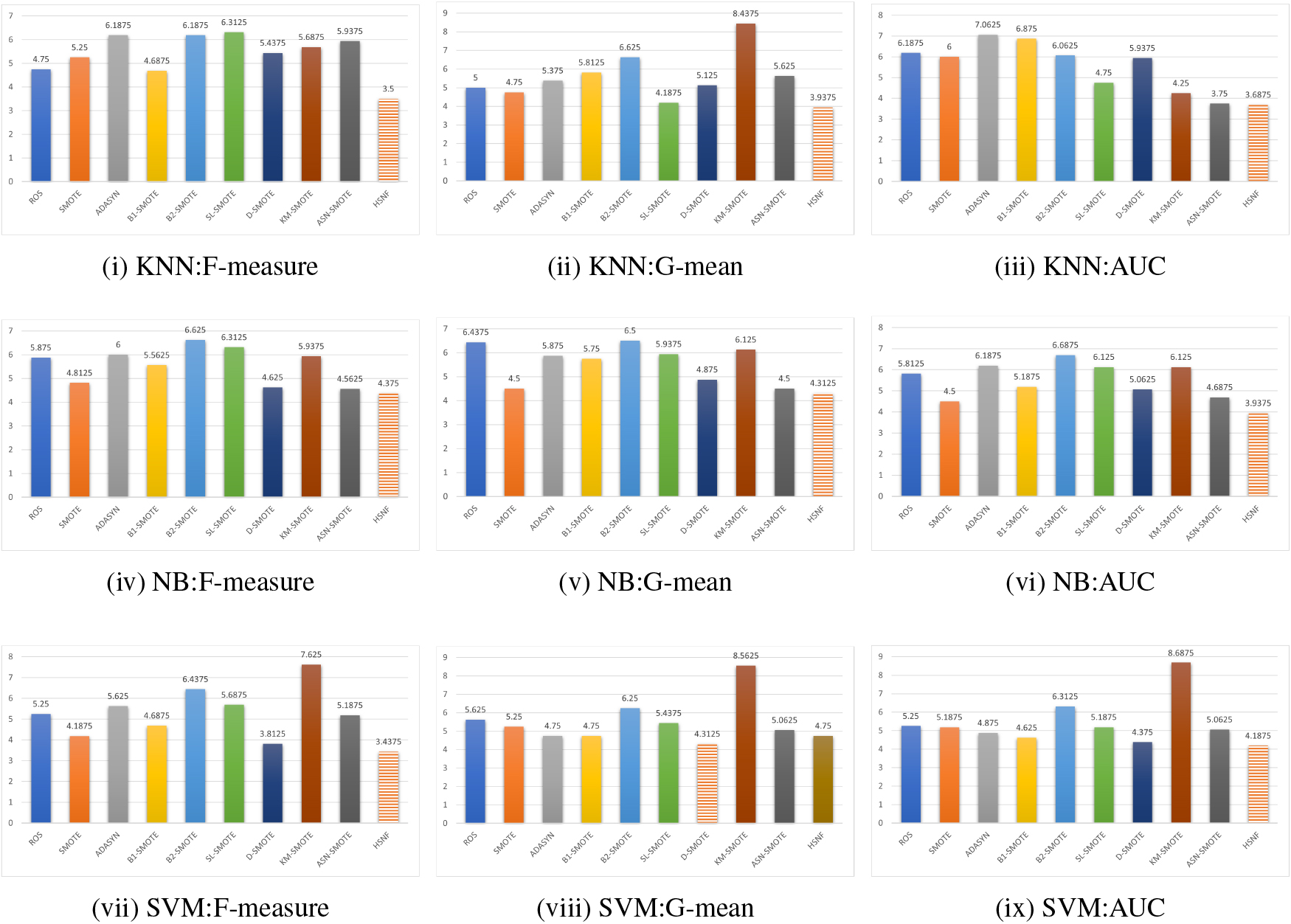

Figure 9.

The trend of classification performance with various 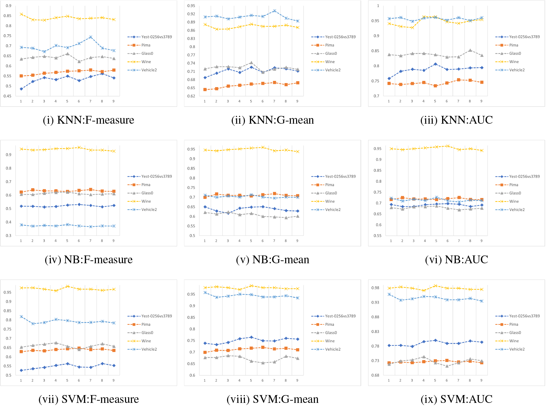$K$ values.

D-SMOTE on G-mean for the highest sum of optimal and suboptimal values. Further, HSNF has the highest ranking on F-measure and AUC, and the second highest ranking on G-mean, but with comparable performance to the highest ranking D-SMOTE (Fig. 8). From Table 11, it can be concluded that the HSNF method significantly outperforms KM-SMOTE on all three measures, and significantly outperforms B2-SMOTE, SLSMOTE and ASN-SMOTE on the F-measure.

In conclusion, HSNF method overall outperforms the comparison method. The reason is that HSNF filters noise more adequately and weakens the influence of noisy samples in the sample synthesis stage; and the HSNF method divides minority samples into categories and uses different oversampling methods to synthesize new samples for them, which reduces the overlap between samples especially between samples of different categories at the boundary and improves the recognition accuracy of minority samples, which in turn improves the overall performance.

4.4.3 Parameter analysis

In our method the parameter $k$ is used, and the parameter $k$ has a significant effect on both the further classification of the minority class samples and the selection of neighbors for the synthetic samples. To investigate the effect of different $k$ values on the performance of our method, we randomly choose five datasets and use KNN, NB and SVM classifier to obtain the values of F-measure, G-mean, and AUC, respectively. As shown Fig. 9, the performance varies with different values of $k$ . In terms of the KNN classifier, taking yest-0-2-5-6_vs_3-7-8-9 dataset as an example, the performance firstly increases with $k$ from 1 to 3, then the performance decrease with $k$ from 3 to 4, and finally, with $k$ from 4 to 9, the performance tends to decrease after reaching a maximum at $k=5$ . In terms of NB classifier, taking wine dataset as an example, the performance firstly decrease with $k$ from 1 to 2, then with $k$ from 2 to 6, the performance increase and reaches a maximum at $k=6$ , and finally, the performance decrease when $k$ increases from 6 to 9. In terms of SVM classifier, taking pima dataset as an example, looking at the overall perspective, the performance increases with $k$ from 1 to 6 and reaches a maximum at $k=6$ , and decreases with $k$ from 6 to 9. Therefore, the optimal $k$ value is different for various classifiers. This shows that we should select a suitable $k$ value when using the HSNF method.

5. Conclusion

In this paper, a hybrid sampling method is proposed for imbalanced data scenarios. Compared with some existing sampling methods, this method not only can filter noise samples sufficiently, it also can synthesize minority class samples with different methods for different minority categories and remove some boundary majority class samples, so as to reduce the overlap between samples. We conducted experiments on 16 datasets with three classifiers and nine sampling methods, and the results indicate that our method outperforms the comparison methods. In the future work, we plan to investigate different noise filtering mechanisms and work on solving multi-class imbalance problems.

Footnotes

Acknowledgments

This work was supported by the Anhui Provincial Natural Science Foundation (Grant No. 2208085 MF168).

References

Lin

W.-C.

Tsai

C.-F.

Y.-H.

and Jhang

J.-S.

, Clustering-based undersampling in class-imbalanced data, Information Sciences 409 (2017), 17–26.

Zakaryazad

and Duman

, A profit-driven artificial neural network (ANN) with applications to fraud detection and direct marketing, Neurocomputing 175 (2016), 121–131.

Zhu

Xia

Jin

Yan

Cai

Yan

and Ning

, Class weights random forest algorithm for processing class imbalanced medical data, IEEE Access 6 (2018), 4641–4652.

Luo

Wang

and Tao

, An improved svm-rfe based on f-statistic and mpdc for gene selection in cancer classification, IEEE Access 7 (2019), 147617–147628.

Engen

Vincent

and Phalp

, Enhancing network based intrusion detection for imbalanced data, International Journal of Knowledge-Based and Intelligent Engineering Systems 12(5–6) (2008), 357–367.

Abdulhammed

Faezipour

Abuzneid

and AbuMallouh

, Deep and machine learning approaches for anomaly-based intrusion detection of imbalanced network traffic, IEEE Sensors Letters 3(1) (2018), 1–4.

Kubat

, Holte

and Matwin

, Machine learning for the detection of oil spills in satellite radar images, Machine Learning 30(2) (1998), 195–215.

Vong

C.-M.

W.-F.

Chiu

C.-C.

and Wong

P.-K.

, Imbalanced learning for air pollution by meta-cognitive online sequential extreme learning machine, Cognitive Computation 7(3) (2015), 381–391.

Azaria

Richardson

Kraus

and Subrahmanian

, Behavioral analysis of insider threat: A survey and bootstrapped prediction in imbalanced data, IEEE Transactions on Computational Social Systems 1(2) (2014), 135–155.

10.

and Garcia

, Learning from imbalanced data, IEEE Transactions on knowledge and Data Engineering 21(9) (2009), 1263–1284.

11.

Weiss

, Mining with rarity: A unifying framework, ACM Sigkdd Explorations Newsletter 6(1) (2004), 7–19.

12.

Ghosh

Bellinger

Corizzo

Branco

Krawczyk

and Japkowicz

, The class imbalance problem in deep learning, Machine Learning, 2022, 1–57.

13.

Fernández

LóPez

Galar

Del Jesus

M.J.

and Herrera

, Analysing the classification of imbalanced data-sets with multiple classes: Binarization techniques and ad-hoc approaches, Knowledge-Based Systems 42 (2013), 97–110.

14.

Batista

G.E.

Prati

R.C.

and Monard

M.C.

, A study of the behavior of several methods for balancing machine learning training data, ACM SIGKDD Explorations Newsletter 6(1) (2004), 20–29.

15.

Sun

Kamel

M.S.

Wong

A.K.

and Wang

, Cost-sensitive boosting for classification of imbalanced data, Pattern Recognition, 40(12) (2007), 3358–3378.

16.

Castro

C.L.

and Braga

A.P.

, Novel cost-sensitive approach to improve the multilayer perceptron performance on imbalanced data, IEEE Transactions on Neural Networks and Learning Systems 24(6) (2013), 888–899.

17.

Lim

Goh

C.K.

and Tan

K.C.

, Evolutionary cluster-based synthetic oversampling ensemble (ECO-ensemble) for imbalance learning, IEEE Transactions on Cybernetics 47(9) (2016), 2850–2861.

18.

Zhao

Jin

Zhang

and Chen

, Multi-class whmboost: An ensemble algorithm for multi-class imbalanced data, Intelligent Data Analysis 26(3) (2022), 599–614.

19.

Hou

and Liu

, An anti-noise ensemble algorithm for imbalance classification, Intelligent Data Analysis 23(6) (2019), 1205–1217.

20.

and Japkowicz

, Class imbalances versus small disjuncts, ACM Sigkdd Explorations Newsletter 6(1) (2004), 40–49.

21.

Mease

Wyner

A.J.

and Buja

, Boosted classification trees and class probability/quantile estimation, Journal of Machine Learning Research 8(3) (2007), 409–439.

22.

Mani

and Zhang

, Knn approach to unbalanced data distributions: A case study involving information extraction, in: Proceedings of Workshop on Learning from Imbalanced Datasets, ICML, vol. 126, 2003, pp. 1–7.

23.

Sun

Yang

Shen

and Qi

, ODOC-ELM: Optimal decision outputs compensation-based extreme learning machine for classifying imbalanced data, Knowledge-Based Systems 92 (2016), 55–70.

24.

Van Hulse

Khoshgoftaar

T.M.

and Napolitano

, Experimental perspectives on learning from imbalanced data, in: Proceedings of the 24th International Conference on Machine learning, 2007, pp. 935–942.

25.

Chawla

N.V.

Bowyer

K.W.

Hall

L.O.

and Kegelmeyer

W.P.

, SMOTE: Synthetic minority over-sampling technique, Journal of Artificial Intelligence Research 16 (2002), 321–357.

26.

Han

Wang

W.-Y.

and Mao

B.-H.

, Borderline-smote: A new over-sampling method in imbalanced data sets learning, in: International Conference on Intelligent Computing, 2005, pp. 878–887.

27.

Bunkhumpornpat

Sinapiromsaran

and Lursinsap

, Safe-level-smote: Safe-level-synthetic minority over-sampling technique for handling the class imbalanced problem, in: Pacific-Asia Conference on Knowledge Discovery and Data Mining, 2009, pp. 475–482.

28.

Bai

Garcia

E.A.

and Li

, ADASYN: Adaptive synthetic sampling approach for imbalanced learning, in: 2008 IEEE International Joint Conference on Neural Networks, IEEE, 2008, pp. 1322–1328.

29.

Krishnamoorthy

and Tang

, ASN-SMOTE: A synthetic minority oversampling method with adaptive qualified synthesizer selection, Complex & Intelligent Systems 8(3) (2022), 2247–2272.

30.

Dudjak

and Martinović

, An empirical study of data intrinsic characteristics that make learning from imbalanced data difficult, Expert Systems with Applications 182 (2021), 115297.

31.

Barua

Islam

M.M.

Yao

and Murase

, MWMOTE-majority weighted minority oversampling technique for imbalanced data set learning, IEEE Transactions on Knowledge and Data Engineering 26(2) (2012), 405–425.

32.

Douzas

Bacao

and Last

, Improving imbalanced learning through a heuristic oversampling method based on k-means and smote, Information Sciences 465 (2018), 1–20.

33.

Bellinger

Sharma

Japkowicz

and Zaïane

O.R.

, Framework for extreme imbalance classification: SWIM – sampling with the majority class, Knowledge and Information Systems 62(3) (2020), 841–866.

34.

De La Calleja

and Fuentes

, A distance-based over-sampling method for learning from imbalanced data sets, in: FLAIRS Conference, 2007, pp. 634–635.

35.

Cover

and Hart

, Nearest neighbor pattern classification, IEEE Transactions on Information Theory 13(1) (1967), 21–27.

36.

Cortes

and Vapnik

, Support-vector networks, Machine Learning 20(3) (1995), 273–297.

37.

Kovács

, Smote-variants: A python implementation of 85 minority oversampling techniques, Neurocomputing 366 (2019), 352–354.

38.

Pedregosa

Varoquaux

Gramfort

Michel

Thirion

Grisel

Blondel

Prettenhofer

Weiss

Dubourg

et al., Scikit-learn: Machine learning in python, Journal of Machine Learning Research 12 (2011), 2825–2830.

39.

Lemaître

Nogueira

and Aridas