Incremental density clustering framework based on dynamic microlocal clusters

Abstract

With the prevailing development of the internet and sensors, various streaming raw data are generated continually. However, traditional clustering algorithms are unfavorable for discovering the underlying patterns of incremental data in time; clustering accuracy cannot be assured if fixed parameters clustering algorithms are used to handle incremental data. In this paper, an Incremental-Density-Micro-Clustering (IDMC) framework is proposed to address this concern. To reduce the succeeding clustering computation, we design the Dynamic-microlocal-clustering method to merge samples from streaming data into dynamic microlocal clusters. Beyond that, the Density-center-based neighborhood search method is proposed for periodically merging microlocal clusters to global clusters automatically; at the same time, these global clusters are updated by the Dynamic-cluster-increasing method with data streaming in each period. In this way, IDMC processes sensor data with less computational time and memory, improves the clustering performance, and simplifies the parameter choosing in conventional and stream data clustering. Finally, experiments are conducted to validate the proposed clustering framework on UCI datasets and streaming data generated by IoT sensors. As a result, this work advances the state-of-the-art of incremental clustering algorithms in the field of sensors’ streaming data analysis.

Keywords

Microlocal cluster incremental clustering micro-cluster big data

1. Introduction

With the rapid development of sensors and network technology, mega data have been collected from social network platforms, intelligent manufacturing, autopilot systems, and e-commercial websites. However, having only large data is not enough, and how to use this crude data effectively is the key to data mining. Therefore, more attention should be given to discovering the valuable information hidden in the data, such as rules, insights, and patterns. Moreover, these pristine data have no labels, which falls under the category of unsupervised learning. Clustering is an effective unsupervised machine-learning algorithm for data mining [1]. It judges the similarity of data according to their predefined attributes and gathers similar samples in the same category. No prior knowledge is required in this process, where only the similarity among the data serves as criteria for clustering. In addition, clustering is a multivariate statistical analysis method [2, 3]. It can show the global distribution of datasets and figure out the relationship among the attributes of data [4].

Information spreading rapidly in the network has become a new form of data flow [5, 6], and this continuous flow of data is on the web all the time. For most enterprises and units, it is impossible to intercept all the network data and save it in the storage medium for unified analysis. On the one hand, hardware resource requirements are very high. On the other hand, network data have a certain timeliness, so the results and knowledge obtained after.

Storing and analyzing the data may be outdated. Discovering the underlying patterns of incremental data in time is an urgent problem to be solved. However, in the face of streaming data, the traditional global clustering algorithm is no longer applicable. An efficient data stream clustering algorithm is needed to analyze the data and feedback on the analysis results in real time [7]. In addition, clustering accuracy cannot be assured if fixed parameter clustering algorithms are used to handle these incremental data [8]. Therefore, clustering methods with fewer or more convenient tuning parameters become more necessary.

Based on this situation, researchers are keen on improving clustering algorithms to cope with the dynamic data environment [9]. For example, the incremental K-means algorithm [10, 11], the incremental clustering algorithm based on Mahalanobis distance [12], and other algorithms have been successively proposed. Guha et al. proposed the stream algorithm [13] to process evolutionary data streams. According to the principle of divide-and-conquer, it uses an iterative process to achieve k-means clustering of data streams in a limited space. Aggarwal et al. proposed a data stream clustering framework Clu-stream [13, 14] based on summarizing the essential defects of the above methods, whose core idea is to divide the clustering process into online and offline stages. Since their core algorithms are still based on K-means, they can only find spherical clusters, and their shortcomings will be exposed when facing nonspherical clusters.

To deal with nonlinear data, especially the arbitrary shape of clusters, a Den-stream clustering algorithm based on density was proposed by Cao et al. [16]. To address this issue, Zhao et al. focused on incremental clustering by extending the clustering by fast search and find of density peaks (DPC) method [17] to incrementally handle large-scale dynamic data [18]. An enhanced version of the incremental Density-Based Spatial Clustering of Applications with Noise (DBSCAN) algorithm was introduced by Bakr et al. [22] for incremental building and updating arbitrary-shaped clusters in large datasets. Bao et al. proposed a boundary-profile-based incremental clustering method to find arbitrarily shaped clusters with dynamically growing datasets [24]. These pure density-based methods have difficulty dealing with inhomogeneous density data, and the adjustment process of multiple parameters is coupled.

In addition, the D-Stream algorithm based on the data flow grid model was proposed by Chen et al. [19]. Chen et al. presented a new type of incremental clustering algorithm [20], which is based on swarm intelligence theory. Suárez et al. introduced a new algorithm for incremental overlapped clustering [21] called Incremental Clustering by Strength Decision. Yu et al. introduced a new incremental soft clustering approach based on three-way decision theory to combat data changes [22]. Nentwig et al. presented new scalable approaches for incremental entity clustering that support the continuous addition of link data [23]. These methods provide a good direction for incremental clustering, but the clustering effect is uneven, and the operation process is complex, which limits their application and promotion.

However, in addition to the computational efficiency that needs to be improved, these algorithms with fixed parameters are unfavorable for discovering patterns from incremental data. To overcome this problem, we propose a two-stage incremental clustering framework Incremental-Density-Micro-Clustering (IDMC), as shown in Fig. 1, which investigates automatic incremental clustering on streaming data from sensors.

Figure 1.

Illustration of our present framework. Dynamic microlocal clustering is the preceding (first) stage of IDMC. With streaming data flowing in, it generates microlocal clusters in real time. Density-center-based neighborhood search and Dynamic-cluster-increasing make up the subsequent (second) stage of IDMC, which integrates all microlocal clusters into final clusters in their ways. In contrast to the other IDMC processes, which run continuously, the density-center-based neighborhood search process runs only after the Dynamic-cluster-increasing given each trigger signal.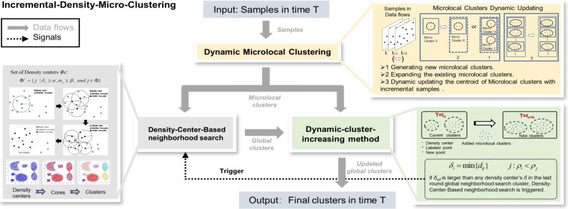

In the first stage, we give a novel definition of density to measure the consistency of each microlocal cluster, and the parameters are adjusted autonomously according to current samples in the streaming dataset. For the incremental clustering setting, we present a dynamic microlocal cluster method in which the centroid is upgraded by the incoming points. Beyond that, an additional parameter is used to enhance the weights and joining degree of the dynamic microlocal cluster. In this way, massive data can be transformed into finite microlocal clusters according to the demands at this step, which can effectively lower the workload in the next stage. At the same time, the new dynamic class cluster data are more accurate than the previous data.

In the second stage, Density-center-based neighborhood searching and Dynamic-cluster-increasing alternate with the incoming microlocal clusters to integrate the final clusters automatically. Density-center based neighborhood searching works as follows. After the density centers of microlocal clusters are selected by their “Megalopolis distance” and density, neighborhood search starts from the highest density one, and all points in its neighbors are classified into the same cluster. This cluster is enlarged by including the neighborhood of merged points until no new neighbor is found. In dynamic clusters increasing, to be specific, the coming microlocal clusters are used for generating new clusters, merging, or dividing existing clusters. After a preset condition is triggered, all microlocal clusters execute another global clustering. These methods make the tuning procedure more convenient and robust, with fewer parameters. Extensive experimental results on eight public datasets and streaming sensor datasets demonstrate the superiority of our framework.

The main contributions of this work are summarized as follows:

As the first step of IDMC, this paper presents a novel Dynamic-microlocal-clustering method in which microlocal clusters are described by dynamic centroids in the data stream, which can effectively lower the workload in the next stage.

The Density-center-based neighborhood search method is utilized as the second stage of IDMC to integrate microlocal clusters to obtain the final clusters automatically. Furthermore, the tuning procedure becomes more convenient and robust with fewer parameters.

We present a Dynamic-cluster-increasing approach that saves time and resources by reclustering fresh samples from the data flow alongside the original data and improving the efficiency of updating real-time global clusters.

The rest of this paper is organized as follows. The preliminary knowledge is introduced in Section 2. We provide the main principles and steps of the IDMC in Section 3. To investigate the performance of the proposed clustering framework, experiments on both UCI real datasets and IoT sensors’ streaming data are presented in Section 4. Finally, conclusions and future studies are discussed in Section 5.

2. Preliminaries

In this section, we introduce some basic principles of related work, including one-pass clustering and DBSCAN clustering. All definitions are based on dataset $D=\{p_{1},p_{2},\ldots,p_{n}\}$ where $p_{i}$ , $i=\{1,2,,n\}$ , is a point in $D$ .

2.1 One-pass clustering

For one-pass clustering, the dataset must be scanned once to accomplish the clustering [24]. It performs well in identifying data with hyper-spherical distributions but poorly in identifying data with convex distributions. Furthermore, it can demonstrate its characteristics of high efficiency and simplicity in large-scale data, secondary clustering, or combination with other algorithms.

The framework is divided into two stages: micro-clustering and ultimate clustering [25]. It constructs an initial local cluster, that is, a micro-cluster reflecting the raw data summary after processing, during the micro-clustering stage. The ultimate clustering is made up of a sequence of interconnected micro-clusters throughout the clustering process.

Micro-clustering is the process of assigning a data point to a micro-cluster. Finding the local cluster all at once creates a micro-cluster with a specific form as the local cluster’s smallest unit. The data points are then assigned successively to micro-clusters to build local clusters.

2.2 Concepts of density clustering

DBSCAN, as a classic density clustering algorithm, gives some essential concepts, especially the definition of density. In it, outlier detection, backbone identification, and density definition depend on the notion of Eps (the cutoff distance) and $\gamma$ (the density threshold) [26].

Neighborhood: If point $i$ is the center and Eps is the radius, all points within the hyper-sphere are the neighborhood of $i$ . $a$ is density-reachable from $b$ , if it is the neighborhood of $b$ .

Density Connected: Two points $a$ and $b$ are density- connected if they are density-reachable from the same point $o$ .

Core point: $\gamma$ is the density threshold, and for point $a$ in $D$ , if $\rho$ ${}_{a}$ > $\gamma$ , then a is a core point.

Border point: Given two points $i$ and $j$ in $D$ , and the density threshold $\gamma$ , $i$ is a border point, if $\rho_{j}>\gamma$ , $\rho_{i}<\gamma$ , and $d_{ij}<\textit{Eps}$ .

Noise point: If point $i$ in $D$ is neither a core nor a border point, it is a noise point.

3. Method

3.1 Dynamic microlocal cluster

Given a sequential dataset $D=\{p_{1},p_{2},\ldots,p_{n}\}$ contains $p_{i}$ , $i=\{1,2,,n\}$ , and $p_{i}^{t}$ is an incoming point with timestamp $t$ . Each of them is allocated to a microlocal cluster as the following definitions.

3.1.1 Microlocal cluster

Let $\varphi$ be the set of points in microlocal cluster, defined as $\varphi_{j}=\{p_{i}|d(p_{i},c_{j})\leq r\}$ , $c_{j}$ is its centroid, and $p_{i}$ is the point that belongs to the microlocal cluster $\varphi_{j}$ . $C$ is the set of all centroids of the $\Phi$ , the set of all $\varphi$ in $D$ . For each microlocal cluster $\varphi_{j}$ , $r$ is the radius of $\varphi_{j}$ and the details about how to select it as shown in Supplementary File 2.1. It represents the granularity of microlocal clusters [27, 28]. $\mu_{\varphi j}(p_{i})$ is the membership value of point $p_{i}$ to microlocal cluster $\varphi_{j}$ ,

$\displaystyle\mu_{\varphi_{j}}(p_{i})=\left\{\begin{array}[]{ll}1,&(p_{i},c_{j% })<d(p_{k},c_{j})<r;\forall k\neq i\\ 0,&\textit{otherwise}\\ \end{array}\right.$ (1)

$\omega_{j}$ is the weight of $\varphi_{j}$ ,

$\displaystyle\omega_{j}=\sum\limits_{i=1}^{n}{\mu_{\varphi_{j}}(p_{i})}$ (2)

$c_{j}$ is the centroid of $\varphi_{j}$ ,

$\displaystyle c_{j}=\frac{\sum\limits_{i=1}^{n}\mu_{\varphi_{j}}(p_{i})\cdot p% _{i}}{\omega_{j}}$ (3)

As the distances between the incoming point and all microlocal clusters are computed for each data point during the microlocal clusters assignment, we can use this information to find adjacent microlocal clusters for final clustering without recomputing the distance between the microlocal clusters. Using the notion of joined microlocal clusters as defined below, the computed distances can continuously track adjacent microlocal clusters.

3.1.2 Dynamic microlocal cluster

For the incremental clustering setting, we present a dynamic microlocal cluster. The centroid $c_{j}$ is upgraded by $m$ incoming points, which add into dynamic microlocal cluster $\varphi_{j}$ at their timestamp. Beyond that, an additional parameter $\lambda$ is used to enhance the weights and joining degree of the dynamic microlocal cluster $\varphi_{j}$ . The value of $\lambda$ is set between 0 and 1, specific certification process is in Supplementary File 2.2. In practical applications, if the data has high timeliness requirements, the value of $\lambda$ is closer to 1; otherwise, it is closer to 0.

$\omega_{j}$ can be written in a recursive form as:

$\displaystyle\omega_{{}_{j}}^{t}=\omega_{{}_{j}}^{t-1}+\sum\limits_{i}^{m}(\mu% _{\varphi_{j}}(p_{i}^{t})+\lambda)$ (4)

The centroid $c_{j}$ will be updated when a new point is added into this $\varphi_{j}$ in the stream data clustering.

$\displaystyle c_{j}^{t}=\frac{c_{j}^{t-1}\cdot\omega_{j}^{t-1}+\sum\limits_{i}% ^{m}{(\mu_{\varphi_{j}}^{t}(p_{i}^{t})+\lambda)\cdot p_{i}^{t}}}{\omega_{j}^{t}}$ (5)

In this way, the late points adding to microlocal clusters can contribute more significantly to their centroids.

3.1.3 Density of microlocal cluster

In order to lay a foundation for final clustering in the following part, we propose a microlocal cluster density calculation. The basic equation is a typical Gaussian kernel and an exponential fading function Date point $p_{i}$ is located in the neighborhood of centroid $c_{j}$ , and $F(p_{i})$ is $p_{i}$ ’s contribution to the density of $c_{j}$ , $e$ is the base of the natural logarithm. The contribution is inversely proportional to the distance between a surrounding point and $j$ . In other words, the density of $\varphi_{i}$ is only sensitive to points near $c_{j}$ .

$\displaystyle F(p)=\frac{1}{e^{p}}$ (6)

Here we give a novel definition of density to measure the consistency of each microlocal cluster, all the parameters are adjusted autonomously according to current microlocal cluster in streaming dataset [29].

Definition 1 (data-bound distance). A data-bound distance of microlocal cluster, $\bar{d}$ is defined as:

$\displaystyle\bar{d}=\frac{1}{n}\sum\limits_{\begin{subarray}{c}p=1\\ q\neq p\end{subarray}}^{n}{\min(d_{pq})}$ (7)

Remark1: $\bar{d}$ is the average distance between all points in $\varphi_{j}$ and their nearest point.

Definition 2 (adaptive density). An adaptive density $\rho_{i}$ is calculated as:

$\displaystyle\rho_{i}=\sum\limits_{j\neq i}^{n}{\frac{1}{e^{\frac{d_{ij}}{% \overline{d}}\cdot r}}}$ (8)

The details of the dynamic microlocal clustering process are shown in Algorithm 3.1.3. First, data points arrive one by one, and the first point $p_{1}$ is treated as $c_{1}$ , the centroid of the first microlocal cluster $\varphi_{j}$ . $\omega_{1}$ , the weight of $\varphi_{j}$ , is 1. The next point calculates the distances between all microlocal cluster centroids in the feature space. For all microlocal clusters whose distance from $p_{i}$ is less than $r$ , if there is no nearby microlocal cluster, $p_{i}$ will be the centroid and generate a new microlocal cluster as line 10. If $\Phi_{p}$ is not empty, the membership value of point $p_{i}$ to its nearest microlocal cluster $\varphi_{j}$ is 1; otherwise, it is 0 using Eq. (1). The $\omega^{t}_{j}$ , $c^{t}_{j}$ , and $\rho^{t}_{j}$ are updated using Eqs (4), (5), and (8).

1em [h] Dynamic microlocal clusteringInputInput InitializationInitialization OutputOutput $p_{i}^{t}$ : incoming data points at timestamp $t$ $r$ : the radius of microlocal cluster. $\Phi_{t}=(\varphi_{1},\ldots,\varphi_{|\Phi|})$ , $\varphi_{j}$ [ $\omega_{j},c_{j},\rho_{j}$ ] $\mu_{1}\leftarrow$ 1, $\varphi_{1}\leftarrow p_{1}$ , $\Phi\leftarrow\varphi_{1}$ Calculate $d(\varphi_{j},p_{i})$ , $\forall\varphi_{j}\in\Phi$ $\Phi_{p}=\{\varphi_{k}|d(p,c_{k})<r\}$ $\Phi_{p}\neq\emptyset$ , for $\varphi_{k}$ in $\Phi_{p}$ : $\mu_{\varphi k}(p_{i})=1,d(p_{i},c_{j})<d(p_{k},c_{j});\forall k\neq i$ $\omega_{j}^{t}=\omega_{j}^{t-1}+\mu_{\varphi_{j}}(p_{i}^{t})+\lambda$ $c_{k}^{t}=\frac{c_{k}^{t-1}\cdot\omega_{k}^{t-1}+(\mu_{\varphi_{k}}^{t}+% \lambda)\cdot p_{i}^{t}}{\omega_{k}^{t}}$ $\rho_{{}_{k}}^{t}=\sum\limits_{j\neq k}^{n}\frac{1}{e^{\frac{d_{kj}}{\overline% {d}}\cdot r}}$ Generate a new microlocal cluster $\varphi_{|\Phi|+1}=\{c_{|\Phi|+1},\omega_{|\Phi|+1}\}$ where $c_{|\Phi|+1}=p,\omega_{|\Phi|}=1$ and $\rho=_{|\Phi|}$

3.2 Density-center-based neighborhood search

3.2.1 Density center selection

In this part, we use a novel method based on density center for executing the clustering process In our work, referred to as “Megalopolis distance” $\delta_{j}$ is calculated by Eq. (9). For point $j$ in dataset $D$ , if $\rho_{j}$ is not the largest then $\delta_{j}$ is the minimum distance between $j$ and other points with a higher density than that of $j$ If $\rho_{j}$ is the largest, $\delta_{j}$ is the maximum distance between $j$ and other points in $D$ .

$\displaystyle\delta_{j}=\min\{d_{ij}\}\quad j:\rho_{j}<\rho_{i}$ (9)

Let us use the megalopolis in Fig. 2 as an analogy to explain the distance $\delta$ . Megalopolis is composed of several large or small cities, and a cluster consists of many samples. The central cities of a megalopolis are like the density centers of clusters, and city size can be likened to $\rho$ , the density of samples.

Figure 2.

Urban distribution in some megalopolises of China and America.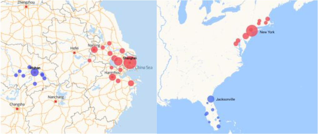

In order to become the central metropolis of a megalopolis, the city must be large enough and far enough away from other larger cities. Shanghai and New York are the central cities of their megalopolis, and there are also many big cities around them, such as Hangzhou and Philadelphia. Because they are adjacent to larger cities, Hangzhou and Philadelphia cannot become the central cities of the megalopolis. However, cities like Wuhan and Jacksonville, comparable in size but far removed from Shanghai and New York, have built megalopoleis around themselves. Therefore, the distance from other larger cities becomes the key to becoming a metropolis. For samples in clustering, megalopolis distance $\delta$ is the key to being a cluster center as well.

$\delta_{j}$ serves as the critical parameter of the microlocal cluster and works in tandem with $\omega_{j}$ , the microlocal cluster’s weight, to select density centers

Definition 3 (density center). Centroids in $C$ satisfy the following conditions and belong to a set of density centers $C^{c}$ :

$\displaystyle C^{c}=\{j|\delta_{j}\geq\alpha,\omega_{j}\geq\beta,\text{and}\ j% \in C\}$ (10)

Where $\alpha$ and $\beta$ are two thresholds that need to be manually set, in our work, the process of density center selection has two steps:

Outlier detection is used on the “Megalopolis distance” of all microlocal clusters. The outlier points can be regarded as preliminary density centers, as shown in Fig. 6c the red points.

When we execute the process of neighborhood searching, the appropriate steps will only run with core points, and the core points refer to centroids whose weight are greater than a certain threshold, i.e., $\varphi_{j}\geq\beta$ , as shown in Fig. 6d, the dark blue triangles. The points that do not meet this condition will be ignored, so preliminary density centers are screened again in this way. So far, the second step of density center selection has been completed.

Identifying density centers is one of the most significant procedures in the neighborhood search of microlocal clusters. If they were not well selected, the final clustering accuracy would be reduced, even leading to a clustering failure. Here, we select the microlocal clusters with large $\delta$ . The larger $\delta$ of a chosen microlocal cluster is the farther it is from other dense ones, and the more likely it is to become a cluster center. $\rho$ of the chosen microlocal cluster also has to be large enough; otherwise, it is likely to be a noisy one. Unlike clustering by fast search and find of density peaks (DPC) [17] what we select are not cluster centers. Because the number of density centers we selected is not equal to the number of final clusters, and we only need to specify the approximate range of their microlocal cluster density centers.

In DPC, cluster centers determine the number of clusters strictly [30]. Hence choosing the parameters of a decision graph is essential. Furthermore, it is extremely difficult to identify cluster centers without previous knowledge of the number of clusters. Because there is no discernible distinction between cluster centers and other nodes on the decision graph, cluster centers should be chosen manually by an expert. These difficulties described above, however, do not bother our algorithm. Furthermore, density centers have the following characteristics:

Density-center-based neighborhood searchInputInput InitializationInitialization OutputOutput $\Phi=(\varphi_{1},\ldots,\varphi_{|\Phi|})$ , $\varphi_{j}[\omega_{j},c_{j},\rho_{j}]$ $\beta$ : The threshold of selecting core microlocal cluster. A microlocal cluster $\varphi_{j}$ whose weight $\omega_{j}$ is larger than $\beta$ is a core cluster.

$\bar{d}(\Phi)$ : The average distance between all points in $\Phi$ with their nearest point. Final clusters Calculate $\delta_{j}$ , $\forall\varphi_{j}\in\Phi$ Outlier detecting in $\delta_{j},\forall\varphi_{j}\in\Phi$ Sorting preliminary density centers by $\rho_{j}$ Selecting core microlocal clusters, for $\varphi_{j}$ in $\Phi$ , if $\omega_{j}>\beta$ Building neighborhoods $i, j$ in $\Phi$ $d_{ij}<\bar{d}(\Phi)$ Set(neighborhood of $i)\leftarrow j$ $i$ in preliminary density centers list $=$ neighborhood of $i$ $j$ in list $j$ in core points $j$ goto cluster $i$ list1 $\leftarrow j$ list $=$ list1 list is disposed all: break Synchronize label of microlocal cluster with its centroid; Output: Clusters

•

Density centers contain cluster centers.

•

The number of density centers is not less than the number of clusters.

•

A density center may be located in the neighborhood of other density centers.

The selection of alpha and beta in Fig. 3 further demonstrates the Density-center-based neighborhood search algorithm’s robustness. It is worth mentioning that the performance of our model is quite stable when alpha and beta is less than 3.5 and 1.5. In practice, selecting parameters should be guided by the simple principleï¼Œi.e., produce as many density centers by keeping alpha and beta values as low as possible. In this case, the clustering accuracies reach a plateau, and the resulting time expenditure is negligible, as shown in Fig. 3(a)–(b). In this way, all these parameter combinations are appropriate.

Figure 3.

The effect of parameters 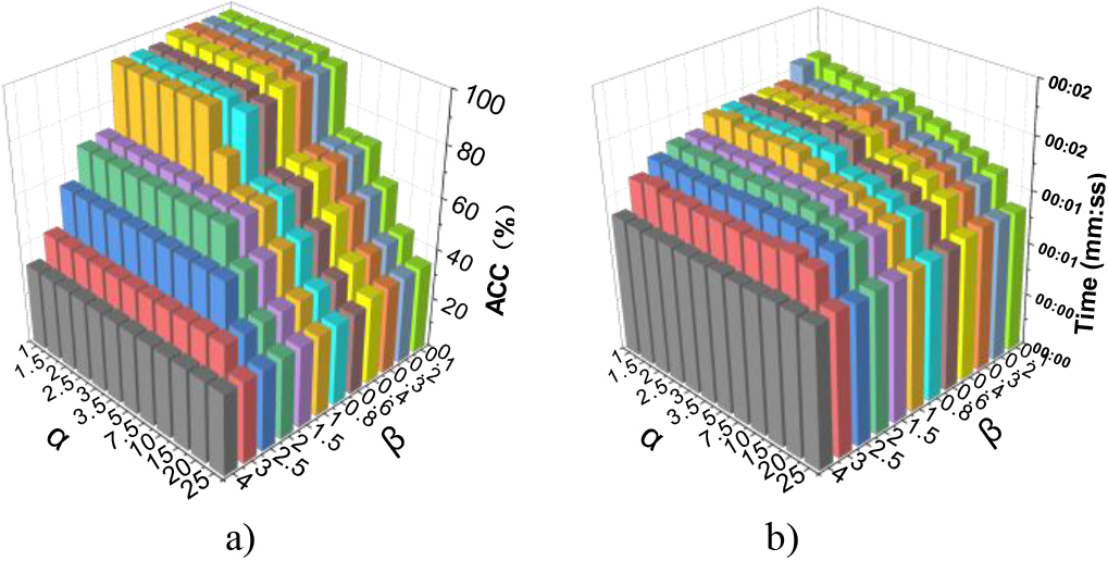$\{\alpha,\beta\}$ on clustering accuracy and execution time on dataset Path-based.

Figure 4.

Processes of neighborhood searching: Starting from the point with the highest density, all the points in the neighborhood are divided into the same cluster. Expand the cluster by merging the neighborhoods of the previously merged points until no new neighbor is found. At this point, we have our first cluster.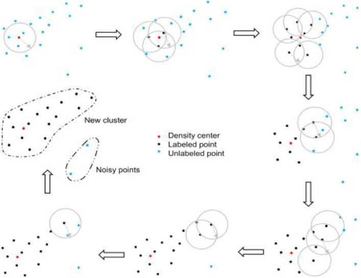

3.2.2 Neighborhood searching

Coalescing by neighborhood search is another crucial step in a clustering process, as shown in Fig. 4. First, the selected density centers are arranged by density. Second, neighborhood search starts from the highest density point, and all points in its neighbors are classified into the same cluster. Third, this cluster is enlarged by including the neighborhood of merged points until no new neighbor is found. Thus, we got the first cluster. In the next round, the following density center will be selected to coalesce the unmerged rest points for seeking another cluster until all density centers are classified. If a point is not merged into any clusters, we regard it as a noise point.

There is a particular situation: a density center $b$ exists in the neighborhood of another density center $a$ . The identity of density center $b$ is ignored and treated as an ordinary point. Specific steps are shown in Algorithm 2.

Finally, the rest points in $\varphi_{j}$ are synchronized with the label of the centroid for each microlocal cluster. So far, all points coming from $D$ are clustered well. All the details are shown in Algorithm 2.

Density-center-based neighborhood search in IDMC shows strong robustness in choosing density centers. In Fig. 5, we use three different schemes (a)-(c) to select density centers. For each operation, such as the scheme of selecting 16 density centers in (a). Ordinary microlocal clusters are dark blue dots and the density centers selected preliminary are shown as red ones in the first graph, wathet dots in the second graph are noisy points, and the clustering result will be shown in the third graph. We can see that the three schemes obtained the same clustering result. Thus, the Density-center-based neighborhood search method has excellent flexibility in selecting density centers. To ensure the accuracy of clustering, it is appropriate to select relatively more density centers at the expense of slightly increased time to execute this approach.

Figure 5.

Three different schemes of density center selection.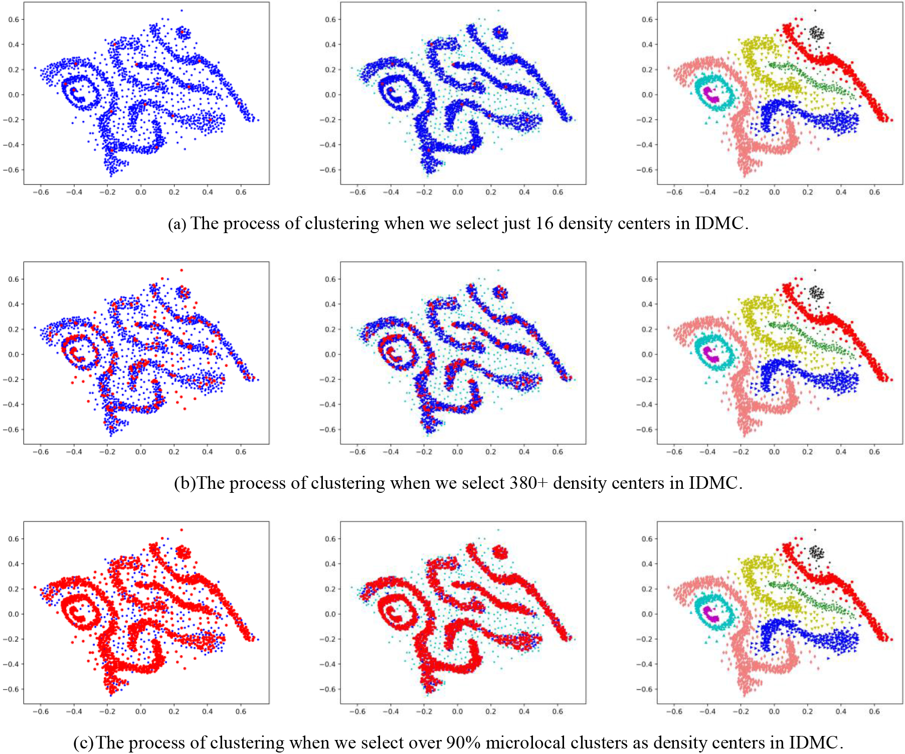

3.3 Dynamic clusters increasing

In this part, each microlocal cluster is coming into global clusters continuously according to their timestamp. To update real-time global clusters and improve our method’s efficiency, we propose a “quantity breeds quality” way to execute the dynamic clusters increase. Specifically, the coming microlocal clusters are usually merged into existing clusters or considered noisy points. After a preset condition is triggered, all microlocal clusters execute Algorithm 2.

At the same time, an exponential fading function $g_{\left(\varphi\right)}$ is used for attenuating the weights of the microlocal clusters $\varphi_{j}$ over time, where $\kappa$ is the decay rate set based on needs, $t$ is the current timestamp, and $T_{\varphi_{j}}$ is the last updated time of microlocal cluster $\varphi_{j}$ .

$\displaystyle g(\varphi_{j})=2^{-\kappa(t-T_{\varphi_{j}})}$ (11)

When a new point does not update a microlocal cluster, its weight will gradually decrease. If the weight of any microlocal cluster is less than a preset threshold, it is removed from the microlocal cluster space $\Phi$ .

[h] Dynamic clusters increasingInputInput InitializationInitialization OutputOutput $\varphi_{t}[\omega_{t},c_{t},\rho_{t}]$ , incoming microlocal cluster at timestamp $t$ ; $\Phi_{t}=(\varphi_{1},\ldots,\varphi_{|\Phi|})$ ; Clusters at timestamp $t$ . $\bar{d}(\Phi_{t})$ : The average distance between all points in $\Phi_{t}$ with their nearest point. Clusters at timestamp $t$ Calculate dist $(\varphi_{j},\varphi_{t}),\forall\varphi_{j}\in\Phi_{t}$ Select list( $\Phi_{t},\varphi_{t}$ ) and Calculate $\delta_{\omega_{t}}$ Applying decay factor to the weight as $\omega_{j}^{t}=g(\varphi_{j})\cdot\omega_{j}^{t}$ $\exists\delta_{j}$ in preliminary density centers $\leq\delta_{\omega_{t}}$ go to Algorithm 2 Min(list( $\Phi_{t},\varphi_{t}))\to\textit{dist}(\varphi_{j},\varphi_{t})$ dist( $\varphi_{j}$ , $\varphi_{t})\leqslant\bar{d}(\Phi_{t})$ $\varphi_{t}\to\textit{cluster of}\varphi_{j}$ $\varphi_{t}\to$ a new cluster Output: Clusters at timestamp $t$

Figure 6.

IDMC’s vital clustering processes of dataset D6.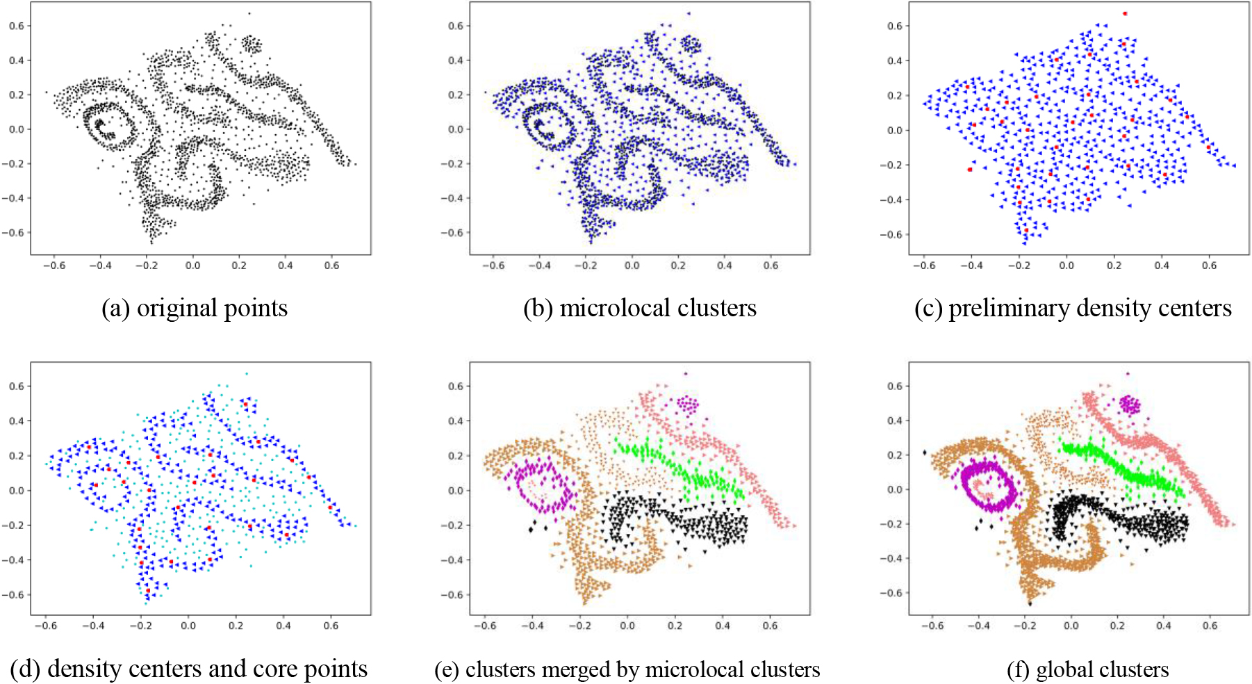

The details of the Dynamic-clusters-increasing process are shown in Algorithm 3.3. First, the distances between incoming microlocal cluster $\varphi_{t}$ and all microlocal clusters are calculated as line 1, then find the distances of $\varphi_{t}$ and each global cluster. $\delta_{\omega_{t}}$ , the “Megalopolis distance” of $\varphi_{t}$ , also needs to be calculated in this step. Second, if $\delta_{\omega_{t}}$ is larger than any density center’s $\delta$ in the last round global neighborhood search cluster, all microlocal clusters will execute Algorithm 2 as line 5. Further, if the situation in line 4 does not appear, incoming microlocal clusters will be merged into a cluster $\varphi_{j}$ when dist( $\varphi_{j}$ , $\varphi_{t})<d(\Phi t)$ as line 9, otherwise, they are classified as noise points as line 11. We revealed the vital processes of IDMC in Fig. 6.

To facilitate the demonstration of the clusters, we adjusted the decay rate $f$ in our experiment to 0 and the radius of the microlocal cluster $r$ to 0.01. It means previously processed microlocal clusters do not lose weight over time, and each microlocal cluster contains just one sample. Figure 7 shows the global clusters in the timestamp of 600, 1000, 1400, and 1800 microlocal clusters. For each batch, microlocal clusters are added into global clusters randomly or sampled by labels. They are merged into original clusters or generated a new one by dynamic clusters increasing method. We find that IDMC can give the global clustering results of the current time automatically. Besides, unabridged artificial experiments supplied in the Supplementary File 4 demonstrate the algorithm’s operation while processing adjacent data.

3.4 Time complexity analysis

For the computational complexity, our framework mainly consists of 3 parts, i.e., Dynamic microlocal clustering, Density-center-based neighborhood search and Dynamic-cluster-increasing. In the first stage, $\tau_{c}=O\left({n\ast\textit{log}_{2}^{n}+n\ast n\left(\Phi\right)}\right)$ , where $n(\Phi)$ denotes the number of microlocal clusters $\Phi$ . In the second stage, $\tau_{s}=O\left({\Phi\ast\textit{log}_{2}^{n\left(\Phi\right)}+n\left(\Phi% \right)}\right)$ . In the last stage, $\tau_{i}=O\left({\left|\textit{Nc}\right|\ast n\left(\Phi\right)}\right)$ , where $N_{C}$ denotes the number of clusters in the end. Thus, the total time complexity is $\tau_{\textit{total}}=\tau_{c}+\tau_{s}+\tau_{i}$ .

Table 1
Synthetic datasets

Dataset	# Samples	# Attributes	# Class
Aggregation	788	2	7
Compound	399	2	6
D8	2,000	2	8
Chameleon T4.8K	8,000	2	6

Figure 7.

Representative dynamic clusters of D6 at different times.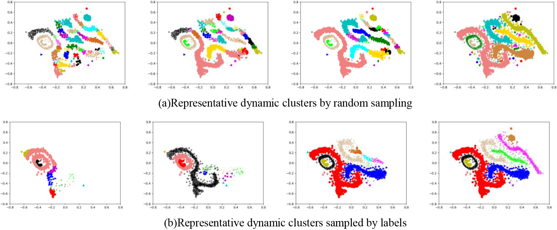

3.4.1 Experiment

In this section, four synthetic and eight UCI real datasets, including mega ones, and streaming data generated by IoT sensors are selected to evaluate the accuracy, efficiency, and adaptability of IDMC with the baselines. Normalized mutual information (NMI) [31], Rand index (RI) [31], and Adjusted Rand index (ARI) [32] were employed as performance indices in all of the studies. The three indices have values ranging from 0 to 1. The higher the values, the greater similarity between the clustering findings and the ground truth. To maintain the values of all characteristics on the same scale across all datasets in the trials, min-max normalization was used to rescale all of the attributes to values between 0 and 1. Besides, all experiments run on Python 3.7 on a laptop with 64-bit Windows, core i5 CPU, and 16 GB of memory.

3.5 Experiment with synthetic datasets

In this part, we show the clustering results of synthetic datasets, IDMC’s outstanding performance in static and incremental data through two-dimensional data with good visibility is highlighted here.

These datasets contain points ranging from 399 to 8000 in two dimensions, representing some intractable clustering instances because they contain clusters with widely different shapes, sizes, and varying densities: 1) Aggregation (Agg) represents a dataset containing arbitrary shaped clusters with uniform density; 2) Compound (Com) represents datasets containing arbitrary shaped clusters with various densities; 3) D8 represents datasets containing concave clusters; 4) Chameleon T4.8K (without labels) represents dataset containing clusters banded non-spherical with shapes. Since T4.8K has no label, the clustering accuracy of this dataset is not presented in Table 2, and only the results of IDMC are given in Fig. 8.

The clustering results of IDMC on the rest synthetic datasets, as shown in Table 2 and Fig. 8 too, show IDMC’s advantages in terms of accuracy and robustness.

Table 2
Final clustering results of IDMC on synthetic datasets

Dataset	NMI	RI	ARI
Aggregation	0.9956	0.9992	0.9978
Compound	0.8974	0.9381	0.8460
D8	0.9255	0.9434	0.9829

Figure 8.

Representative dynamic clusters of aggregation compound and chameleon T4.8K.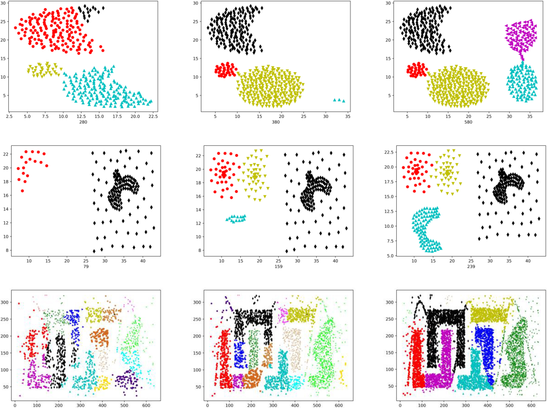

3.6 Experiment with UCI real datasets in traditional data clustering setting

The second section of the experiment is the performance of IDMC on the static dataset of UCI. Because the upper limit of the accuracy of the performance of the incremental clustering algorithm is static clustering, that is, the accuracy of the dataset when it is read into the clustering algorithm all at once is higher than that when the data is read into the clustering algorithm in batches. Therefore, after obtaining its remarkable clustering effect on synthetic datasets, we continue to use IDMC on UCI real datasets and compare it with other state-of-the-art traditional clustering algorithms, including DBSCAN [26], HDBSCAN [33], DPC [17], SNN-DPC [34], FKNN-DPC [35], and EvolveCluster [36]. The experimental data are taken from seven different datasets in the UCI database (http://archive.ics.uci.edu/ml/), a database for machine learning presented by the University of California at Irvine. Each dataset contains a different number of samples, attributes, and classes with strong typicality and universality. Table 3 lists the description of seven multi-dimensional datasets.

Table 3
Real datasets for evaluating clustering performance with traditional clustering algorithms

Dataset	# Samples	# Attributes	# Class
Image segmentation	2,310	19	7
Land sat	4,435	36	7
Pen-based digit	7,494	16	10
Spambase	4,601	57	2
Multiple features	2,000	649	10
Waveform	5,000	21	3
Waveform-noise	5,000	40	3

The cluster accuracy results of IDMC in this set of experiments are shown in Table 4. The clustering accuracy of the comparison algorithm FIDC comes from [37]. One of the input parameters of the DPC family algorithms, including EvolveCluster, DPC, SNN-DPC, and FKNN-DPC was the number of clusters. As a result, the total number of final and ground truth clusters must always be the same. This might give these algorithms a leg up on their competition.

Table 4

Comparison of clustering performances on real datasets

Datasets	Algorithms	NMI	ARI	RI	Parameters
Image segmentation	IDMC	0.7561	0.5921	0.9570	$r=$ 0.15
	FIDC	0.7445	0.5376	0.9459	$r=$ 0.08
	SNN-DPC	0.7013	0.5770	0.9007	$k=$ 7
	FKNN-DPC	0.5629	0.4151	0.8182	$k=$ 21
	DPC	0.7264	0.6004	0.9127	$d_{c}=$ 1.5
	DBSCAN	0.6393	0.4386	0.8730	Eps,MinPts $=$ 0.15,5
	HDBSCAN	0.7365	0.5853	0.9353	MinPts $=$ 5
	EvolveCluster	0.6528	0.4716	0.9010	$k=$ 5
Land sat	IDMC	0.8166	0.6390	0.9349	$r=$ 0.3
	FIDC	0.7971	0.5760	0.9342	$r=$ 0.13
	SNN-DPC	0.6976	0.7023	0.9014	$k=$ 9
	FKNN-DPC	0.5661	0.4203	0.7478	$k=$ 19
	DPC	0.5356	0.4080	0.8243	$d_{c}=$ 1.2
	DBSCAN	0.6157	0.3760	0.6825	Eps,MinPts $=$ 0.34,5
	HDBSCAN	0.6987	0.4765	0.8041	MinPts $=$ 5
	EvolveCluster	0.5477	0.4129	0.8014	$k=$ 8
Pen-based digit	IDMC	0.8768	0.7743	0.9883	$r=$ 0.2
	FIDC	0.8654	0.7744	0.9726	$r=$ 0.17
	SNN-DPC	0.7262	0.5524	0.9041	$k=$ 4
	FKNN-DPC	0.7035	0.5348	0.8969	$k=$ 26
	DPC	0.7256	0.5896	0.9233	$d_{c}=$ 0.4
	DBSCAN	0.7112	0.5408	0.9113	Eps,MinPts $=$ 0.15,5
	HDBSCAN	0.8515	0.7591	0.9672	MinPts $=$ 5
	EvolveCluster	0.8117	0.7414	0.9413	$k=$ 6
Spambase	IDMC	0.7498	0.6629	0.9450	$r=$ 0.01
	FIDC	0.7041	0.6464	0.9337	$r=$ 0.075
	SNN-DPC	0.0113	0.0063	0.5185	$k=$ 10
	FKNN-DPC	–	–	–	–
	DPC	0.0166	0.0327	0.5301	$d_{c}=$ 1.3
	DBSCAN	0.5354	0.6082	0.89221	Eps,MinPts $=$ 0.15,7
	HDBSCAN	0.1494	0.1852	0.5693	MinPts $=$ 20
	EvolveCluster	0.5117	0.4514	0.6522	$k=$ 10
Multiple features	IDMC	0.9080	0.7605	0.9242	$r=$ 3
	FIDC	0.9168	0.7757	0.9784	$r=$ 2.5
	SNN-DPC	0.7548	0.6232	0.9236	$k=$ 7
	FKNN-DPC	0.4917	0.2105	0.6317	$k=$ 19
	DPC	0.8262	0.7193	0.9425	$d_{c}=$ 0.1
	DBSCAN	0.7013	0.4473	0.8739	Eps,MinPts $=$ 5.7,4
	HDBSCAN	0.9067	0.7332	0.9636	MinPts $=$ 7
	EvolveCluster	0.7051	0.7014	0.9324	$k=$ 4
Waveform	IDMC	0.6212	0.4593	0.8792	$r=$ 0.5
	FIDC	0.6014	0.4470	0.8726	$r=$ 0.44
	SNN-DPC	0.3983	0.4176	0.7381	$k=$ 7
	FKNN-DPC	0.0405	0.0086	0.6130	$k=$ 6
	DPC	0.3352	0.2698	0.7012	$d_{c}=$ 0.1
	DBSCAN	0.1350	0.0097	0.5312	Eps,MinPts $=$ 0.38,5
	HDBSCAN	0.5575	0.4282	0.8340	MinPts $=$ 3
	EvolveCluster	0.5641	0.4754	0.6544	$k=$ 6
Waveform-noise	IDMC	0.4125	0.3312	0.7256	$r=$ 0.8
	FIDC	0.4481	0.3708	0.7467	$r=$ 0.82
	SNN-DPC	0.3199	0.3108	0.6512	$k=$ 10
	FKNN-DPC	0.0670	0.0125	0.4287	$k=$ 6
	DPC	0.0981	0.0695	0.5123	$d_{c}=$ 2.1
	DBSCAN	–	–	–	–
	HDBSCAN	–	–	–	–
	EvolveCluster	0.1354	0.1014	0.2314	$k=$ 6

In Table 4, in most datasets, IDMC yields the best performance indices than its peers. It generates the best performance indices for the majority of datasets except for Multiple features and Waveform-noise. These two data sets contain a large number of noise points, so the compactness of various clusters is not enough, and the boundary between classes is not apparent, which leads to the difficulty of IDMC in neighborhood search and reduces the accuracy of clustering. Nevertheless, fuzzy local clustering is employed in FIDC to reduce clustering inconsistencies so that it surpasses the compared algorithms in these two datasets. DBSCAN and HDBSCAN rejected more than half of the Waveform (noise) datasets as outliers. Consequently, these two methods are considered to fail to handle these datasets.

In order to verify the superiority of IDMC, a statistical test for the comparison in Table 4 was performed using nonparametric tests for multiple comparisons. Friedman test [38] is a nonparametric equivalent of the repeated-measures ANOVA, and it is a commonly used test to compare the overall performance of $k$ algorithms on $N$ datasets.

$\displaystyle\chi_{F}^{2}=\frac{12N}{k(k+1)}\left[{\sum\limits_{j}{R_{j}^{2}-% \frac{k(k+1)^{2}}{4}}}\right]$ (12)

$R_{j}$ is the average rank of the algorithm, $R_{j}=\frac{1}{N}\sum_{i}r_{i}^{j}$ . Under the null hypothesis, which states that all the algorithms are equivalent, their ranks $R_{j}$ should be equal. In the Friedman test critical value table, we select $F_{0.05}$ [8,7] $=$ 3.726 for experiments with less methods and data sets, including ours. From the average ranks of three performance indices of each dataset in Table 5, we get $\chi_{F}^{2}=$ 34.6 $>$ 3.726.

Table 5

Ranks and $p$ -values of the compared algorithms for the benchmark datasets

Dataset	IDMC	FIDC	SNN-DPC	FKNN-DPC	DPC	DBSCAN	HDBSCAN	EvolveCluster
Image segmentation	1	4	5	8	3	7	2	6
Land sat	1	2	3	7	5	8	4	6
Pen-based digit	1	2	6	8	5	7	3	4
Spambase	1	2	7	8	6	3	5	4
Multiple features	3	1	6	8	4	7	2	5
Waveform	1	2	5	8	6	7	3	4
Waveform-noise	2	1	3	5	4	7.5	7.5	6
Everge rank	$1.42$	$2.00$	$5.00$	$7.43$	$4.71$	$6.64$	$3.78$	$5$
P-values		0.33	$0.003$	$0.00$	$0.0057$	$0.00$	$0.0084$	$0.003$
Critical values		0.05	$0.01$	$0.0083$	$0.0167$	$0.01$	$0.025$	$0.011$

Iman and Davenport [39] showed that Friedman’s $\chi_{F}^{2}$ is undesirably conservative and derived a better statistic which is distributed according to the F-distribution with 6 and 36 degrees of freedom. We get $F_{F}=$ 14.42 $>$ $F_{0.05[6,36]}=$ 2.364. The null hypothesis is rejected at a high level of significance, so the performances of the compared algorithms have significant statistical differences.

$\displaystyle F_{F}=\frac{(N-1)\chi_{F}^{2}}{N(k-1)-\chi_{F}^{2}}$ (13)

Friedman test can only give the conclusion of whether there is a difference in the performance of $k$ algorithms. So, a “post hoc test” is needed to find out which algorithms have statistical differences in performance. The test statistics for comparing the $i$ -th and $j$ -th classifier using these methods is

$\displaystyle z={(R_{i}-R_{j})}\mathord{\left/{\vphantom{{(R_{i}-R_{j})}{\sqrt% {\frac{k(k+1)}{6N}}}}}\right.\kern-1.2pt}{\sqrt{\frac{k(k+1)}{6N}}}$ (14)

$z$ is used to find the corresponding probability from the $N$ (0,1) typical distribution table. In our experiments, $N=$ 7, $k=$ 8, and get $\alpha=$ 0.05. We use IDMC as the control algorithm. $P$ -values are calculated according to each $z$ value of the comparison algorithm by the Holm procedure. Table 5 shows the $P$ -values and their critical values. All $P$ -values except FIDC are less than their corresponding critical values, which means these hypotheses are rejected, indicating that IDMC outperformed these algorithms with statistical significance. The $P$ -values of FIDC are less than its critical values, which means our method and FIDC are not significantly different, and they outperform other state-of-the-art peers.

3.7 Comparison of computation time and performance indices on large scale sensors dataset

With the development of the Internet of Things, the number of sensors increases, which puts forward higher requirements for the algorithm’s computing power on large-scale data. We validate the efficiency of IDMC by comparing it with the traditional clustering method, by selecting the Phones-accelerometer dataset, a sub dataset of “Heterogeneity Activity Recognition,” to verify the arithmetic speed of IDMC on a mega dataset. It contains the readings of two motion sensors commonly found in smartphones. Readings were recorded while users executed activities scripted in no specific order carrying smartwatches and smartphones. It contains 1,048,576 samples, eight attributes, and seven classes.

Table 6
Comparison of computation time on large scale datasets

IDMC ( $r=$ 1.5)
Size	Time (h:mm:ss)	NMI	RI
10,000	0:00:05	0.34848	0.4446
20,000	0:00:09	0.36291	0.4840
30,000	0:00:13	0.35620	0.4935
40,000	0:00:18	0.36210	0.5321
50,000	0:00:24	0.35807	0.5261
60,000	0:00:26	0.36282	0.5443
70,000	0:00:33	0.35756	0.5342
80,000	0:00:37	0.35991	0.5553
90,000	0:00:45	0.36191	0.5442
100,000	0:00:49	0.36587	0.5379
200,000	0:01:54	0.3417	0.4726
300,000	0:03:11	0.3659	0.5199
400,000	0:04:25	0.3662	0.5148
500,000	0:05:41	0.3655	0.4973
600,000	0:07:23	0.3665	0.5069
700,000	0:08:55	0.3508	0.4437
800,000	0:10:28	0.3574	0.4944
900,000	0:11:59	0.3419	0.4591
1,000,000	0:13:45	0.3541	0.4898
DBSCAN (Eps $=$ 0.1, Minpts $=$ 5)
10,000	0:00:13	0.3650	0.4736
20,000	0:00:32	0.3751	0.4835
30,000	0:01:05	0.3473	0.5000
40,000	0:01:53	0.3208	0.5061
50,000	0:02:50	0.3114	0.5018
60,000	0:04:03	0.3037	0.4932
70,000	0:05:30	0.2977	0.4925
80,000	0:07:21	0.2945	0.4729
90,000	0:10:13	0.2915	0.4827
100,000	0:14:26	0.2945	0.4768

${}^{*}$ Mega data is too tricky for DPC-family and HDBSCAN, relatively efficient DBSCAN is chosen as the benchmark.

Figure 9.

Comparison of execution time on the large-scale dataset.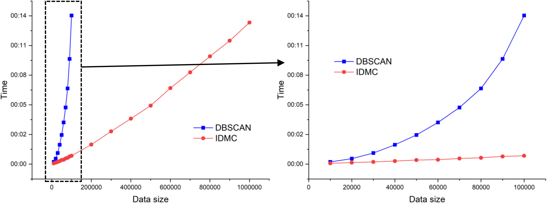

Figure 10.

Photovoltaic generation system and sensors.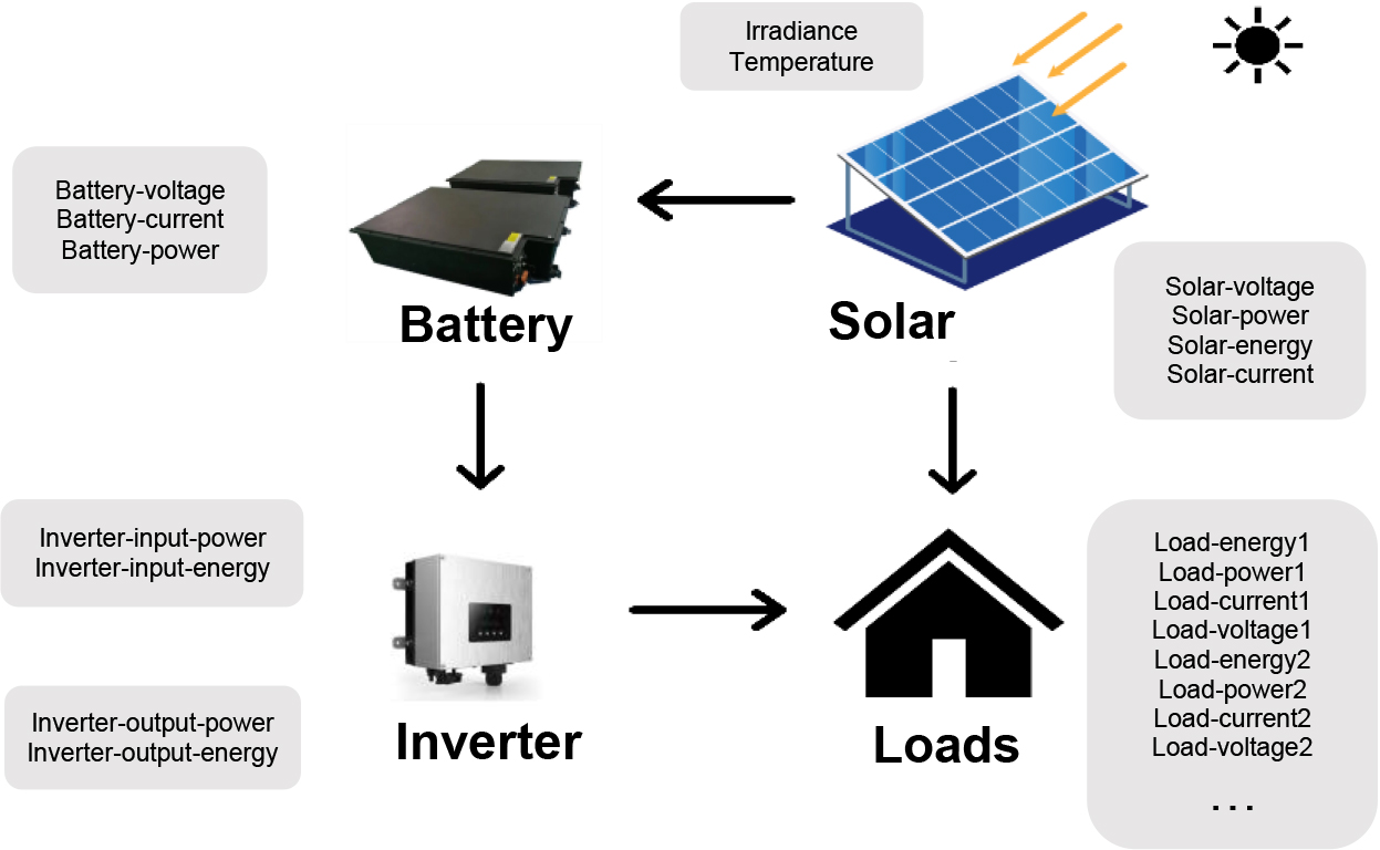

Because DPC-family algorithms are incapable of handling datasets larger than 10,000 samples, we did not use them for experiments. As HDBSCAN is also incapable of dealing with large datasets, DBSCAN is the only method to handle large datasets efficiently. We randomly selected 100,000 to 1,000,000 samples without replacement from the phones-accelerometer dataset. The computation time and performance indices for each algorithm are kept track. For each sample size, Table 6 displays the average findings of 10 repetitions.

During the experiment, we discovered that DBSCAN’s operating speed is one order of magnitude slower than IDMC. So, we chose the data volume of DBSCAN from 10000 to 100000, as in Table 6 and Fig. 9, to better compare the running time of the display method. Moreover, we discovered that the running time of IDMC is basically linearly proportional to the quantity of data, while that of DBSCAN is exponential. Because we used dynamic microlocal clusters to represent the uniformly distributed but numerous samples in the first stage of IDMC; in the second stage, we used a “quantity breeds quality” principle to reduce the number of Epochs on microlocal clusters. As a consequence, our algorithm has a significant advantage when dealing with large-scale data. Furthermore, despite more data to process, IDMC’s clustering accuracy is higher.

3.8 Application in streaming sensors data

In this part, we apply IDMC to data stream from a photovoltaic power system for comparison with Clu-stream [13], DenStream [40], DBSTREAM [41], StreamKM++ [42], and Dstream [19], not only to compare the running speed, but also the real-time clustering accuracy. This data is acquired by sensors as part of each working operation and is timestamped. All dataset in this section is derived from [25]. Photovoltaic power generation is a burgeoning industry that is widely promoted as a sustainable energy alternative. The batteries, inverter, and other equipment are connected to the solar panels as shown in Fig. 10. They charge batteries and power load devices on sunny days. At night and on overcast days, batteries provide electricity to loads.

Sensors are installed above and below solar panels, as well as in the batteries, inverter, and load subsystems. They record the voltage, instantaneous power, and current of the solar panels, batteries, and each load. Sensors placed above the solar panels record the temperature and irradiance of the panels (sun exposure). There are 119266 rows and 23 columns in this dataset. Except for “date-time” and “location,” all variables are numeric. Solar panels, batteries, inverters, and loads are the four components. The samples of this dataset are recorded every one minute.

Table 7
Comparison of results on solar panel sensors

	IDMC				Clu-stream
Size	Time (s)	NMI	ARI	RI	Time (s)	NMI	ARI	RI
10,000	0:02.37	0.8534	0.6564	0.9420	0:03.73	0.8481	0.5963	0.9271
20,000	0:05.03	0.8554	0.6548	0.9421	0:07.12	0.8408	0.5958	0.9192
30,000	0:07.90	0.8557	0.6536	0.9418	0:09.77	0.8315	0.5941	0.9135
40,000	0:10.19	0.8555	0.6533	0.9413	0:13.81	0.8356	0.5948	0.9135
50,000	0:13.79	0.8541	0.6539	0.9414	0:16.10	0.8306	0.5931	0.9161
60,000	0:17.40	0.8556	0.6556	0.9416	0:20.07	0.8374	0.5952	0.9242
70,000	0:19.65	0.8564	0.6557	0.9421	0:22.08	0.8401	0.5962	0.9234
80,000	0:24.22	0.8557	0.6551	0.9416	0:25.56	0.8323	0.5943	0.9218
90,000	0:26.93	0.8572	0.6535	0.9424	0:28.01	0.8341	0.5954	0.9116
100,000	0:31.42	0.8565	0.6541	0.9420	0:33.95	0.8432	0.5968	0.9157
110,000	0:35.31	0.8557	0.6562	0.9416	0:37.28	0.8462	0.597	0.9272
	DenStream				Dstream
Size	Time (s)	NMI	ARI	RI	Time (s)	NMI	ARI	RI
10,000	00:02.21	0.8406	0.6466	0.9260	00:01.68	0.8496	0.6329	0.9373
20,000	00:05.84	0.8380	0.6421	0.9286	00:05.00	0.8373	0.6271	0.9222
30,000	00:11.26	0.8409	0.6433	0.9269	00:11.05	0.8348	0.6293	0.9319
40,000	00:10.44	0.8410	0.6433	0.9285	00:28.02	0.8383	0.6301	0.9312
50,000	00:15.47	0.8390	0.6430	0.9265	00:40.37	0.8332	0.6277	0.9303
60,000	00:19.31	0.8450	0.6481	0.9302	00:58.87	0.8459	0.6353	0.9411
70,000	00:23.72	0.8411	0.6446	0.9272	01:10.38	0.8406	0.6303	0.9305
80,000	00:30.50	0.8404	0.6441	0.9257	01:23.92	0.8347	0.6289	0.9317
90,000	00:37.36	0.8400	0.6416	0.9260	01:47.40	0.8334	0.6277	0.9277
100,000	00:39.62	0.8427	0.6446	0.9320	02:16:33	0.8449	0.6324	0.9235
110,000	00:39.41	0.8455	0.6489	0.9384	02:42.37	0.8524	0.6366	0.9272
DBSTREAM				StreamKM++
Size	Time (s)	NMI	ARI	RI	Time (s)	NMI	ARI	RI
10,000	00:01.02	0.843428	0.651359	0.934605	00:00.71	0.849142	0.626234	0.927563
20,000	00:05.02	0.843799	0.645386	0.938502	00:04.11	0.841462	0.621497	0.928193
30,000	00:12.06	0.842532	0.650719	0.933015	00:12.43	0.837176	0.624114	0.92348
40,000	00:27.76	0.842338	0.649216	0.938955	00:24.66	0.84342	0.624157	0.926627
50,000	00:44.30	0.839938	0.646901	0.93726	00:51.78	0.836941	0.626975	0.92561
60,000	01:10.30	0.851639	0.650424	0.936258	01:15.01	0.851416	0.628003	0.923522
70,000	01:25.59	0.843938	0.647975	0.933861	01:31.03	0.84192	0.623064	0.926249
80,000	01:41.79	0.842596	0.651146	0.933864	01:48.49	0.839827	0.622006	0.928559
90,000	02:02.84	0.841547	0.643349	0.938829	02:13.04	0.838815	0.623745	0.927215
100,000	02:19.98	0.845009	0.650392	0.935826	02:26.02	0.841941	0.626457	0.923594
110,000	02:47.83	0.852254	0.652521	0.937515	02:46.10	0.847809	0.628616	0.923462

Figure 11.

Comparison of clustering results on streaming data of solar panel sensors.

Figure 12.

Comparison of clustering results on streaming data of loads sensors.

Table 8

Comparison of results on loads sensors

	IDMC				Clu-stream
Size	Time (s)	NMI	ARI	RI	Time (s)	NMI	ARI	RI
10,000	00:07.74	0.3432	0.3506	0.6308	00:05.28	0.3200	0.3092	0.5284
20,000	00:16.94	0.4757	0.4233	0.7003	00:10.16	0.4355	0.3813	0.6106
30,000	00:27.05	0.4781	0.4278	0.7105	00:34.57	0.4233	0.3682	0.5870
40,000	00:38.18	0.5691	0.4766	0.7549	00:49.76	0.4915	0.4036	0.6159
50,000	00:52.04	0.4959	0.4356	0.7141	01:52.80	0.3683	0.3337	0.5474
60,000	01:02.81	0.4813	0.4231	0.6942	02:03.04	0.3931	0.3439	0.5506
70,000	01:16.31	0.4327	0.3975	0.6715	02:53.56	0.3580	0.3276	0.5410
80,000	01:30.56	0.5185	0.4461	0.7207	03:55.12	0.4829	0.3984	0.6103
90,000	01:38.72	0.5387	0.4605	0.7405	04:28.65	0.4339	0.3740	0.5923
100,000	01:54.91	0.5498	0.4764	0.7737	05:04.18	0.4484	0.3907	0.6235
110,000	02:11.65	0.5432	0.4586	0.7308	05:30.30	0.3554	0.3285	0.5460
	DenStream				Dstream
Size	Time (s)	NMI	ARI	RI	Time (s)	NMI	ARI	RI
10,000	00:12.1	0.3431	0.3117	0.5582	0:00:12	0.3026	0.3480	0.4823
20,000	00:26.4	0.4201	0.3673	0.6559	0:00:45	0.3621	0.3685	0.5174
30,000	00:42.9	0.4478	0.3090	0.6404	0:01:34	0.4125	0.3743	0.5194
40,000	00:59.0	0.4829	0.3520	0.6949	0:02:06	0.4275	0.4308	0.6108
50,000	01:16.0	0.4542	0.3243	0.6219	0:03:53	0.4241	0.4066	0.6059
60,000	01:32.0	0.4664	0.3396	0.6269	0:04:56	0.4567	0.4298	0.6525
70,000	01:47.0	0.4295	0.3123	0.5864	0:06:22	0.4191	0.3950	0.5988
80,000	02:03.0	0.4506	0.3280	0.6394	0:08:10	0.4053	0.4036	0.5797
90,000	02:24.0	0.4666	0.3299	0.6253	0:10:24	0.4268	0.4121	0.6098
100,000	02:41.0	0.4595	0.3573	0.6674	0:13:17	0.3964	0.4251	0.5663
110,000	02:59.0	0.4441	0.3623	0.6700	0:16:27	0.3715	0.4213	0.5308
	DBSTREAM				StreamKM++
Size	Time (s)	NMI	ARI	RI	Time (s)	NMI	ARI	RI
10,000	00:18.7	0.4278	0.3566	0.6541	00:45.4	0.4005	0.3191	0.6993
20,000	00:25.8	0.351	0.3376	0.6561	00:54.8	0.4373	0.3573	0.6554
30,000	00:53.1	0.441	0.3634	0.6704	01:05.2	0.4111	0.328	0.6836
40,000	01:02.1	0.3568	0.3923	0.6091	01:15.6	0.402	0.3269	0.6501
50,000	01:09.7	0.4336	0.349	0.6177	01:19.6	0.4573	0.3562	0.6392
60,000	01:14.6	0.3623	0.3635	0.6513	01:40.2	0.4058	0.3281	0.6127
70,000	01:28.9	0.3685	0.3191	0.6344	01:53.5	0.4091	0.358	0.6112
80,000	01:51.4	0.379	0.3217	0.637	01:58.6	0.4058	0.3477	0.6502
90,000	02:16.1	0.427	0.3552	0.6011	02:26.1	0.4832	0.3999	0.6475
100,000	02:21.8	0.3798	0.323	0.6675	02:31.7	0.4205	0.331	0.7046
110,000	02:37.0	0.4233	0.314	0.6383	02:44.2	0.4309	0.3595	0.6512

For the photovoltaic power system, we perform a cluster comparison using the sensor data of solar panels. It has five characteristics; all samples are periodically and significantly correlated with solar activity. The evaluation window for the performance indices is set at 10,000 points. The computation time and accuracy are averaged from the results of 10 experiments. From Fig. 12, we find the NMI of four algorithms can reach 80% in the first batch and maintained at that level throughout, which indicates the data from solar panels sensors are in periodic variation and static modes. As a result, all algorithms can detect hidden patterns and distinguish them using distinct clusters. Apart from that, IDMC surpasses the comparison method in every performance metric. The clustering accuracy is more stable and will not vary significantly with the increase of the number of samples.

We implement cluster comparison on additional data collected by load sensors. It contains six characteristics, and the pattern is more intricate and unpredictable, changing with the season, time, weather, and other factors. The evaluation window for performance indices is also set at 10,000 points. In Fig. 12(a), the time spent by IDMC increases in a conventional linear manner as the data volume increases. The computation time of the other three algorithms, on the other hand, is much higher than that of IDMC, Dstream’s execution time, in particular, does not follow a traditional linear relationship with data size. Because the data instances are so distributed, the resulting clusters exhibit a low degree of homogeneity, as seen in Fig. 12(b)–(d). However, IDMC surpasses the other algorithms in all performance indexes. Overall, IDMC outperforms its competitors in robustness, execution speed, and accuracy.

3.9 Experimental analysis and summary

All of the above are the four main parts of the experiment. Part A shows IDMC’ outstanding performance on artificial datasets. IDMC’s outstanding performance in static and incremental data through two-dimensional data with good visibility is highlighted here. The second part of the experiment is the performance of IDMC on the static dataset of UCI. Because the upper limit of the accuracy of the performance of the incremental clustering algorithm is static clustering, that is, the accuracy of the dataset when it is read into the clustering algorithm all at once is higher than that when the data is read into the clustering algorithm in batches. Therefore, in this part, we compare the accuracy of the IDMC algorithm with the classic and efficient clustering baselines, which proves that IDMC has strength over the traditional static clustering algorithm when dealing with static data. The third section of the experiment is to compare the speed of IDMC and traditional clustering algorithms. With the development of the Internet of Things, the number of sensors increases, which puts forward higher requirements for the algorithm’s computing power on large-scale data. DBSCAN is a traditional clustering algorithm and its ability to deal with large-scale data is the best, so in this part, we compare it with IDMC for operation speed, and the results can see the advantages of our algorithm on large-scale datasets. The fourth section is the comparison experiment between IDMC and dynamic clustering algorithms. We compare IDMC with three excellent dynamic clustering algorithms. From the tables and pictures, we can see that our method can not only compare the running speed but also the real-time clustering accuracy. As a result, our IDMC framework advances the state-of-the-art of incremental clustering algorithms in the field of sensors’ streaming data analysis.

4. Conclusion

For streaming sensor data, we suggested an incremental density clustering framework based on dynamic microlocal clusters. As the foundational step of IDMC, we use a novel Dynamic microlocal clustering method in which microlocal clusters are described by dynamic centroids in the data stream. Then, Density-center-based neighborhood searching and Dynamic cluster increasing methods alternate with the incoming microlocal clusters to integrate microlocal clusters to get the final clusters automatically. IDMC processed sensor data with less computational time and memory, improved the clustering performance, and simplified the parameter choosing in conventional and stream data clustering. Furthermore, parameters tuning procedures become more convenient and robust. Extensive experiment results on eight public datasets and streaming sensors dataset demonstrate the superiority of our framework. In future work, we plan to extend IDMC in three respects. Firstly, a built-in feature reduction algorithm will be integrated into the algorithm to perform feature reduction and clustering simultaneously. Secondly, solving other tasks, such as classification, fusion, regression, etc. [43, 44] is an interesting future work. Besides, we will operate IMDC in a distributed clustering environment [45] to accommodate very larger volume datasets.

Footnotes

Acknowledgments

This work was supported by the National Natural Science Foundation of China (61991413) and Science Fund for Creative Research Groups of the National Natural Science Foundation of China (61821005) and Supported by the Joint Funds of the National Natural Science Foundation of China (U22B2041) and National Natural Science Foundation of China (91948303) and the Local science and technology projects guided by the central government of Liaoning Province (2022JH6/100100009).

References

Kaufman

and Rousseeuw

P.J.

, Finding groups in data: an introduction to cluster analysis, vol. 344. John Wiley & Sons, 2009.

Qin

Huang

and Ke

, Damage Localization of Stacker’s Track Based on EEMD-EMD and DBSCAN Cluster Algorithms, IEEE Trans Instrum Meas 69(5) (2020), 1981–1992. doi: 10.1109/TIM.2019.2919375.

Wang

Zhu

Gao

and Sun

, Bearing Fault Diagnosis Based on Clustering and Sparse Representation in Frequency Domain, IEEE Trans Instrum Meas 70 (2021), 1–14. doi: 10.1109/TIM.2021.3067657.

She

Zeng

Wang

and Xu

, Adaptive fuzzy C-means clustering integrated with local outlier factor, Intell Data Anal 26(6) (2022), 1507–1521. doi: 10.3233/IDA-216266.

Jain

A.K.

, Data clustering: 50 years beyond K-means, Pattern Recognit Lett 31(8) (2010), 651–666.

Zhang

Zhu

Yang

L.T.

Chen

Zhao

and Li

, An Incremental CFS Algorithm for Clustering Large Data in Industrial Internet of Things, IEEE Trans Ind Inform 13(3) (2017), 1193–1201. doi: 10.1109/TII.2017.2684807.

Hsu

P.-Y.

and Nguyen

P.-A.-H.

, A fast method for discovering suitable number of clusters for fuzzy clustering, Intell Data Anal 26(6) (2022), 1523–1538. doi: 10.3233/IDA-200511.

Fong

Harmouche

Narasimhan

and Antoni

, Mean Shift Clustering-Based Analysis of Nonstationary Vibration Signals for Machinery Diagnostics, IEEE Trans Instrum Meas 69(7) (2020), 4056–4066. doi: 10.1109/TIM.2019.2944503.

Wang

Chen

and Mei

J.-P.

, Incremental fuzzy clustering with multiple medoids for large data, IEEE Trans Fuzzy Syst 22(6) (2014), 1557–1568.

10.

Chakraborty

and Nagwani

N.K.

, Analysis and Study of Incremental K-Means Clustering Algorithm, in High Performance Architecture and Grid Computing, Berlin, Heidelberg, 2011, pp. 338–341. doi: 10.1007/978-3-642-22577-2_46.

11.

Chakraborty

and Nagwani

N.K.

, Analysis and study of incremental k-means clustering algorithm, in International Conference on High Performance Architecture and Grid Computing, 2011, pp. 338–341.

12.

Aik

L.E.

and Choon

T.W.

, An incremental clustering algorithm based on Mahalanobis distance, AIP Conference Proceedings 1635(1) (2014), 788–793.

13.

Guha

Meyerson

Mishra

Motwani

and O’Callaghan

, Clustering data streams: Theory and practice, IEEE Trans Knowl Data Eng 15(3) (2003), 515–528.

14.

Friedman

Goaz

and Rottenstreich

, Clustreams: Data Plane Clustering, in Proceedings of the ACM SIGCOMM Symposium on SDN Research (SOSR), 2021, pp. 101–107.

15.

Aggarwal

C.C.

Philip

S.Y.

Han

and Wang

, A framework for clustering evolving data streams, in Proceedings 2003 VLDB conference, 2003, pp. 81–92.

16.

Cao

Estert

Qian

and Zhou

, Density-based clustering over an evolving data stream with noise, in Proceedings of the 2006 SIAM international conference on data mining, 2006, pp. 328–339.

17.

Rodriguez

and Laio

, Clustering by fast search and find of density peaks, Science 344(6191) (2014), 1492–1496.

18.

Zhao

Chen

Yang

Zou

and Wang

Z.J.

, ICFS Clustering With Multiple Representatives for Large Data, IEEE Trans Neural Netw Learn Syst 30(3) (2019), 728–738. doi: 10.1109/TNNLS.2018.2851979.

19.

Chen

and Tu

, Density-based clustering for real-time stream data, in Proceedings of the 13th ACM SIGKDD international conference on Knowledge discovery and data mining, 2007, pp. 133–142.

20.

Chen

and Meng

Q.-C.

, An incremental clustering algorithm based on swarm intelligence theory, in Proceedings of 2004 International Conference on Machine Learning and Cybernetics (IEEE Cat. No.04EX826), 2004, vol. 3, pp. 1768–1772. doi: 10.1109/ICMLC.2004.1382062.

21.

Suárez

A.P.

Trinidad

J.F.M.

Ochoa

J.A.C.

and Medina Pagola

J.E.

, A New Incremental Algorithm for Overlapped Clustering, in Progress in Pattern Recognition, Image Analysis, Computer Vision, and Applications, 2009, pp. 497–504. doi: 10.1007/978-3-642-10268-4_58.

22.

Zhang

and Hu

, An Incremental Clustering Approach Based on Three-Way Decisions, in Rough Sets and Current Trends in Computing, 2014, pp. 152–159. doi: 10.1007/978-3-319-08644-6_16.

23.

Nentwig

and Rahm

, Incremental Clustering on Linked Data, in 2018 IEEE International Conference on Data Mining Workshops (ICDMW), 2018, pp. 531–538. doi: 10.1109/ICDMW.2018.00084.

24.

Laohakiat

Phimoltares

and Lursinsap

, A clustering algorithm for stream data with LDA-based unsupervised localized dimension reduction, Inf Sci 381 (2017), 104–123. doi: 10.1016/j.ins.2016.11.018.

25.

Jiang

Pang

and Kuang

, An improved K-nearest-neighbor algorithm for text categorization, Expert Syst Appl 39(1) (2012), 1503–1509. doi: 10.1016/j.eswa.2011.08.040.

26.

Ester

Kriegel

H.-P.

Sander

and Xu

, A density-based algorithm for discovering clusters in large spatial databases with noise, Kdd 96(34) (1996), 226–231.

27.

Laohakiat

Phimoltares

and Lursinsap

, A clustering algorithm for stream data with LDA-based unsupervised localized dimension reduction, Inf Sci 381 (2017), 104–123.

28.

Laohakiat

Phimoltares

and Lursinsap

, Hyper-cylindrical micro-clustering for streaming data with unscheduled data removals, Knowl-Based Syst 99 (2016), 183–200. doi: 10.1016/j.knosys.2016.02.004.

29.

Zhang

Zhou

Guo

and Qi

, A Density-center-based Automatic Clustering Algorithm for IoT Data Analysis, p. 17.

30.

Wang

Tian

and Song

, Belief Density Peak Clustering Algorithm for Uncertain Data, Inf Control Inf Contrl, pp. 1–10.

31.

Manning

C.D.

Raghavan

and Schütze

, Introduction to Information Retrieval, New York: Cambridge University Press Inc, 2008.

32.

Vinh

N.X.

Epps

and Bailey

, Information theoretic measures for clusterings comparison: Variants, properties, normalization and correction for chance, J Mach Learn Res 11 (2010), 2837–2854.

33.

Campello

R.J.

Moulavi

Zimek

and Sander

, Hierarchical density estimates for data clustering, visualization, and outlier detection, ACM Trans Knowl Discov Data TKDD 10(1) (2015), 1–51.

34.

Liu

Wang

and Yu

, Shared-nearest-neighbor-based clustering by fast search and find of density peaks, Inf Sci 450 (2018), 200–226.

35.

Ding

and Jia

, Study on density peaks clustering based on k-nearest neighbors and principal component analysis, Knowl-Based Syst 99 (2016), 135–145.

36.

Nordahl

Boeva

Grahn

and Persson Netz

, EvolveCluster: an evolutionary clustering algorithm for streaming data, Evol Syst 13(4) (2022), 603–623. doi: 10.1007/s12530-021-09408-y.

37.

Laohakiat

and Sa-ing

, An incremental density-based clustering framework using fuzzy local clustering, Inf Sci 547 (2021), 404–426. doi: 10.1016/j.ins.2020.08.052.

38.

Sheldon

M.R.

Fillyaw

M.J.

and Thompson

W.D.

, The use and interpretation of the Friedman test in the analysis of ordinal-scale data in repeated measures designs, Physiother Res Int 1(4) (1996), 221–228. doi: 10.1002/pri.66.

39.

Pereira

D.G.

Afonso

and Medeiros

F.M.

, Overview of Friedman’s Test and Post-hoc Analysis, Commun Stat – Simul Comput (2015), Accessed: Dec. 28, 2021. doi: 10.1080/03610918.2014.931971.

40.

Cao

Estert

Qian

and Zhou

, Density-based clustering over an evolving data stream with noise, in Proceedings of the 2006 SIAM international conference on data mining, 2006, pp. 328–339.

41.

Hahsler

and Bolaños

, Clustering Data Streams Based on Shared Density between Micro-Clusters, IEEE Trans Knowl Data Eng 28(6) (2016), 1449–1461. doi: 10.1109/TKDE.2016.2522412.

42.

Ackermann

M.R.

Märtens

Raupach

Swierkot

Lammersen

and Sohler

, StreamKM++: A clustering algorithm for data streams, ACM J Exp Algorithmics 17 (2012), doi: 10.1145/2133803.2184450.

43.

Zhang

Cong

Sun

Dong

Liu

and Ding

, Generative Partial Visual-Tactile Fused Object Clustering, ArXiv Prepr. ArXiv201214070, 2020.

44.

Zhang

Cong

Sun

and Dong

, Visual-Tactile Fused Graph Learning for Object Clustering, IEEE Trans Cybern, 2021.

45.

Talmale

and Shrawankar

, Cluster Based Real Time Scheduling for Distributed System, ADCAIJ Adv Distrib Comput Artif Intell J 10(2), Art. no. 2, Mar. 2021, doi: 10.14201/ADCAIJ2021102137156.

Incremental density clustering framework based on dynamic microlocal clusters

Abstract

Keywords

1. Introduction

2.1 One-pass clustering

2.2 Concepts of density clustering

3. Method

3.1 Dynamic microlocal cluster

3.1.1 Microlocal cluster

3.2.1 Density center selection

Table 1 Synthetic datasets

3.5 Experiment with synthetic datasets

Table 2 Final clustering results of IDMC on synthetic datasets

Table 3 Real datasets for evaluating clustering performance with traditional clustering algorithms

Table 6 Comparison of computation time on large scale datasets

Table 7 Comparison of results on solar panel sensors

4. Conclusion

Footnotes

Acknowledgments

References

Table 1
Synthetic datasets

Table 2
Final clustering results of IDMC on synthetic datasets

Table 3
Real datasets for evaluating clustering performance with traditional clustering algorithms

Table 6
Comparison of computation time on large scale datasets

Table 7
Comparison of results on solar panel sensors