Using eigenvalues of distance matrices for outlier detection

Abstract

Distance or dissimilarity matrices are widely used in applications. We study the relationships between the eigenvalues of the distance matrices and outliers and show that outliers affect the pairwise distances and inflate the eigenvalues. We obtain the eigenvalues of a distance matrix that is affected by $k$ outliers and compare them to the eigenvalues of a distance matrix with a constant structure. We show a discrepancy in the sizes of the eigenvalues of a distance matrix that is contaminated with outliers, present an algorithm and offer a new outlier detection method based on the eigenvalues of the distance matrix. We compare the new distance-based outlier technique with several existing methods under five distributions. The methods are applied to a study of public utility companies and gene expression data.

Keywords

Distance matrix decomposition eigenvalue outlier detection

1. Introduction

The aim of this article is to study distance matrices, their eigenvalue structures and offer a distance-based outlier detection method. Given $m$ independent vectors ${\bf X}_{1},{\bf X}_{2},\ldots,{\bf X}_{m}$ in $\mathbb{R}^{p}$ from an unknown distribution ${F}$ with mean ${\bm{\mu}}$ and covariance matrix ${\bm{\Sigma}}$ , we would like to find the outliers in the data set and assess their significance. Outliers are those anomalous observations that are inconsistent with or deviate from the rest of the observations. Outliers are often due to measurement and recording errors or formation of new and smaller clusters. Hence, outliers contain valuable information about the target population and the data collection process. However, one also needs to consider that natural variation can also produce outliers. Outliers adversely affect model selection and parameter estimation. Once outliers are identified one can carry the analysis with and without outliers to study their effects. Let $k$ be the number of possible outliers in the data set. To differentiate between the outliers and the non-outliers we must ensure $k<\lfloor\frac{m}{2}\rfloor$ . Outliers can have unfavorable effects on the sample mean and covariance and cause outlier masking (not all outliers are identified) and outlier swamping (non-outlying observations are incorrectly labeled as outliers).

Outlier detection methods find applications in finance, machine learning, clustering, quality control, hot-spot detection, early warning earthquake and tsunami systems, geographic information system, fraud detection, environmental statistics and public health. With a long history in Statistics and applications many researchers have worked on methods of outlier detection [4]. Hadi et al. [11] present an overview of the methods of outlier detection. Leva and Paganoni [8] propose a new method for detecting outliers in multivariate functional data. Cabana Lillo and Laniado [6] present a collection of robust Mahalanobis distances for multivariate outlier detection, based on the notion of shrinkage. While model-based multivariate outlier detection methods exist they are dependent on correct specification of the distribution of the observations. Another approach is proximity-based or distance-based techniques that utilize the spatial proximity of the observations. Modarres [22] uses a high dimensional dissimilarity index to detect outliers as $p\to\infty$ .

Outlier detection is often the goal of the analysis and the focus is on discovering the outlying observations and learning about the unknown aspects of the data. In order to determine which if any of the observations are aberrations one cannot order the observations unambiguously when $p>2$ . Depth functions provide an approach for identifying the usual data points, i.e. observations with small or zero depth values. However, different depth functions produce different probability contours and outliers. To assess the significance of a suspect outlier model-based methods compute the probability of its occurrence under the specified model. Nonparametric bootstrap of the data matrix provides the sampling distribution of a test statistic for outlier detection under the hypothesis of no outliers.

As a measure of similarity, the Euclidean distance is affected by the scales of measurement of the different variables. For example, given $X_{1}=(10000,1)$ and $X_{2}=(10100,5)$ , the Euclidean distance between $X_{1}$ and $X_{2}$ will be dominated by the first component although it only changes 1%. To overcome this difficulty it is common practice in outlier detection to standardize the variables by dividing each by its sample standard deviation or other robust scale measures. When the variables have different units or variances that are of different orders of magnitude it is sensible to standardize the variables. We standardize the variables so as to equalize the effect of variables with differing variances.

A popular outlier detection method uses the Mahalanobis distance [18]. It uses the sample mean vector $\bar{\bf X}$ and the sample covariance matrix $\bf S$ to compute $M({\bf X})=m({\bf X}-{\bar{\bf X}})^{\prime}\bf{S}^{-1}({\bf X}-{\bar{\bf X}})$ , where $\bf X$ is a $p$ -variate vector of the observations. As $m\to\infty$ one can approximate $M$ with a $\chi^{2}(p)$ distribution. The mean vector has a zero breakdown point and is a non-robust measure of multivariate location. Hence, the Mahalanobis distance is non-robust. The method also requires the inverse of the sample covariance matrix, which is undefined when $p>m$ . When $p<m$ minimum covariance determinant and the minimum volume ellipsoid [25] are used to obtain robust estimators of the mean and the covariance. Another approach searches for outliers along data projections that maximize or minimize the kurtosis coefficient [24].

It is much easier to detect outliers by visual inspection. However, this method only works when $1\leqslant p\leqslant 3$ . For higher dimensional data, most outlier detection methods reduce dimensionality by projecting the data into lower dimensions. Detection of multivariate outliers is more challenging when $p>m$ since an observation can be a non-outlier in lower dimensions, but an outlier in $p$ -dimensional space. Hence, marginal, pairwise or three dimensional plots of the observations may fail to reveal outliers in higher dimensions. Working with the norm of all pairwise differences of observations, interpoint distances (IPDs) project the observations to one dimension and provide a versatile tool when $p>m$ . Modarres and Song [21] present a recent survey of IPDs, and Guo and Modarres [10] use IPDs for classification. Modarres [20] proposes methods for visualization and comparison of high dimensional observations.

We propose a nonparametric method that uses the distance matrix instead of the data matrix to detect multivariate outliers. When $p>m$ the distance matrix provides a significant dimension reduction. As a Distance-based outlier detection method, the proposed technique searches for outliers through the $m\times m$ distance matrix instead of the $m\times p$ observation matrix. The matrix of distances has smaller dimensions than the data matrix and does not grow with $p$ . Our approach remains feasible when $p>m$ .

Since outliers inflate the eigenvalues of the distance matrix our approach obtains the eigenvalues of the distance matrix and uses them for outlier detection. Given an $m\times m$ data matrix, our test statistic is the largest eigenvalue of the observed distance matrix. We remove one observation at a time from the data set, extract the reduced data matrix, and compute its largest eigenvalue. This provides us with a list of $m$ largest eigenvalues. The suspect outlier is the observation ${\bf X}_{t}$ , the removal of which provides the greatest reduction in the eigenvalues. We establish that with $k$ outliers in the data set, after the outliers are removed sequentially, the remaining outliers no longer inflate the eigenvalues of the reduced matrix and the algorithm terminate.

The article is organized as follows. In Section 2, we discuss distance matrices, obtain the eigenvalues of a constant distance matrix and a distance matrix is contaminated with $k$ outliers. We show a discrepancy in the sizes of the first $k$ eigenvalues and the remaining eigenvalues. Section 3 describes an algorithm called ODD (Outlier Detection using Distances) and provide several examples. Section 4 compares the performance of ODD against several existing outlier detection methods. The final section is devoted to summary and recommendations .

2. Distance matrix

Let $\|\mathbf{X}\|=(\mathbf{X}^{\prime}\mathbf{X})^{\frac{1}{2}}$ be norm of $\mathbf{X}$ . Consider i.i.d. vectors $\mathbf{X}_{i}$ and $\mathbf{X}_{j}$ from ${\mathbb{F}}$ . The IPD between $\mathbf{X}_{i}$ and $\mathbf{X}_{j}$ is given by $d_{ij}=\|\mathbf{X}_{i}-\mathbf{X}_{j}\|$ . The distance matrix ${\bf D}({\mathbb{X}})$ is an $m\times m$ symmetric matrix with zeros on the main diagonal and $d_{ij}$ on the off-diagonal, $i\neq j=1,\ldots,m$ . In a sample of $m$ independent vectors $\mathbf{X}_{i}$ , there are $m(m-1)/2$ IPDs, of which any two IPDs $d_{ij}$ and $d_{i^{\prime}j^{\prime}}$ are said to be independent if and only if $(i,j)\neq(i^{\prime},j^{\prime})$ . IPDs are asymptotically pairwise independent as $m$ becomes large [27]. Consider the symmetric matrix of distances ${\bf D}(\mathbb{X})$ with elements $d_{ij}$ when $i\neq j$ and zero on the main diagonal,

$\displaystyle{\bf D}(\mathbb{X})=\bordermatrix{&X_{1}&X_{2}&X_{3}&\ldots&X_{m}% \cr X_{1}&0&d_{12}&d_{13}&\dots&d_{1m}\cr X_{2}&d_{21}&0&d_{23}&\ldots&d_{2m}% \cr X_{3}&d_{31}&d_{32}&0&\ldots&d_{3m}\cr&\dots&\dots&\dots&\ldots&\ldots\cr X% _{m}&d_{m1}&d_{m2}&d_{m3}&\ldots&0\cr}.$ (1)

The expected distance matrix ${\mathbb{E}}({\bf D}(\mathbb{X}))$ has zero diagonal entries and off-diagonal elements ${\mathbb{E}}(d_{ij})={\mathbb{E}}\|{\bf X}_{i}-{\bf X}_{j}\|$ . The Euclidean distance geometry problem seeks to construct the configuration of the data matrix given information on pairwise IPDs. Gower [9] introduced the principal coordinate analysis, the aim of which is to retrieve the original observation matrix by performing an eigenvalue decomposition on the distance matrix [19]. This method is invariant with respect to translation and rotation. Denote by $I_{m}$ the identity matrix of order $m$ and by $J_{m}={\bf 1}_{m}{\bf 1}^{\prime}_{m}$ the $m\times m$ matrix of 1’s. To perform a singular value decomposition of distance matrices for construction of the the original observations, the following steps are taken in Algorithm 1.

[h] Decomposition of distance matricesStep 1: Let ${\mathbf{P}}={\bf I}_{m}-{\bf J}_{m}/m$ be an $m\times m$ centering matrix Step 2: Let ${\bf D}=(d_{ij})$ and ${\mathbf{A}}=(a_{ij})$ where $a_{ij}=-\frac{1}{2}d_{ij}^{2}$ for $i\neq j=1,\ldots,m$ Step 3: Let ${\mathbf{B}}={\mathbf{P}}\ {\mathbf{A}}\ {\mathbf{P}}$ , with eigenvalues ${\bm{\Lambda}}={\text{d}iag}(\lambda_{1},\ldots,\lambda_{m})$ , and eigenvectors ${\bm{\Gamma}}=(\mathbf{\gamma}_{1},\ldots,\mathbf{\gamma}_{m})$ . Assuming $\lambda_{1}\geqslant\lambda_{2},\ldots,\lambda_{m-1}\geqslant\lambda_{m}$ , we have ${\mathbf{B}}={\bm{\Gamma}}{\bm{\Lambda}}{\bm{\Gamma}}$ Step 4: Given the $m\times p$ data matrix $\mathbf{X}$ , we have ${\mathbf{X}}{\mathbf{X}}^{\prime}={\mathbf{B}}={\bm{\Gamma}}{\bm{\Lambda}}{\bm% {\Gamma}}$ . Let $\bf X$ denote the $m\times p$ data matrix. It is well known that the non-zero eigenvalues of $m{\bf S}$ and ${\bf B}={\bf PAP}$ are the same. Since $m{\bf S}={\bf X}^{\prime}{\bf PX}=({\bf PX}^{\prime})({\bf PX})$ and ${\bf B}={\bf PX}{\bf X}^{\prime}{\bf P}=({\bf PX})({\bf PX})^{\prime}$ it follows that ${\bf B}={\bf H}{\bm{\Delta}}{\bf H}^{\prime}$ and $n{\bf S}={\bf Q}{\bm{\Delta}}{\bf Q}^{\prime}$ where ${\bf H}$ is a $m\times p$ column orthogonal matrix and $\bf Q$ is a $p\times p$ orthogonal matrix.

Consider the $m\times m$ symmetric distance matrix

$\displaystyle{\bf D}(\mathbb{X})=d\left[\begin{array}[]{ccccc}0&1&1&\ldots&1\\ 1&0&1&\ldots&1\\ \vdots&\vdots&\vdots&\vdots\\ 1&1&1&\dots&0\end{array}\right],$ (2)

It is not difficult to show that its eigenvalues are $\lambda_{i}=\frac{1}{2}d^{2}$ for $i=1,\ldots,m-1$ and $\lambda_{m}=0$ . To study an alternative to the constant distance matrix suppose the distance between the first $k$ and the remaining observations scaled by $c$ with $c>0$ while the the rest of the observations are equidistant. Consider the distance $m\times m$ matrix with $k$ outliers represented as the first $k$ rows of the distance matrix

$\displaystyle{\bf D}(\mathbb{X})=\bordermatrix{&X_{1}&X_{2}&\ldots&X_{k}&X_{k+% 1}&\ldots&X_{m}\cr X_{1}&0&cd&cd&cd&cd&\ldots&cd\cr X_{2}&cd&0&cd&cd&cd&\ldots% &cd\cr{\vdots}&\vdots&\vdots&\vdots&\vdots&\vdots&\vdots&\vdots\cr X_{k}&cd&% \ldots&cd&0&cd&\ldots&cd\cr X_{k+1}&cd&\ldots&cd&cd&0&\ldots&d\cr{\vdots}&% \vdots&\vdots&\vdots&\vdots&\vdots&\vdots\cr X_{m}&cd&\ldots&cd&cd&d&\ldots&0% \cr},$ (3)

where the remaining $m-k$ observations are equidistant. It is not difficult to show that the eigenvalues of ${\bf D}(\mathbb{X})$ are

$\displaystyle\lambda_{1}=\frac{1}{2}d^{2}\left[\frac{(k+1)(m-k)}{m}c^{2}-\frac% {k(m-k-1)}{m}\right],$ $\displaystyle\lambda_{2}=\ldots=\lambda_{k}=\frac{1}{2}d^{2}c^{2},$ (4) $\displaystyle\lambda_{k+1}=\ldots=\lambda_{m-1}=\frac{1}{2}d^{2},$ $\displaystyle\lambda_{m}=0,$

where eigenvalues have multiplicities of $1,(k-1),(m-k-1)$ and $1$ , respectively. To ensure $\lambda_{1}>\lambda_{2}$ we must have $\frac{(k+1)(m-k)}{m}c^{2}-\frac{k(m-k-1)}{m}>c^{2}$ or $c^{2}>\frac{k(m-k-1)}{(k+1)(m-k)+m}$ . To ensure $\lambda_{k}>\lambda_{k+1}$ we must have $c^{2}>1$ ; otherwise, the order of eigenvalues $\lambda_{2}=\ldots=\lambda_{k}$ switches with $\lambda_{k+1}=\ldots=\lambda_{m-1}$ . When there is only $k=1$ outlier in the sample, Eq. (2) reduces to

$\displaystyle\lambda_{1}=\frac{1}{2}d^{2}\left[\frac{2(m-1)}{m}c^{2}-\frac{(m-% 2)}{m}\right],\quad\lambda_{2}=\ldots=\lambda_{m-1}=\frac{1}{2}d^{2},\quad% \lambda_{m}=0.$ (5)

While the above distance matrix is specific to $k$ shift/scale outliers it serves to show that the outliers inflate the eigenvalues of the distance matrix.

The following example describes the effects of shift/scale on one outlier. Consider the distance matrix where the distance between the first and the remaining observations is scaled by $c$ and shifted by $a>0$ with $c\neq 0$ while the rest of the observations are equidistant.

$\displaystyle D(\mathbb{X})=\begin{bmatrix}0&cd+a&cd+a&\ldots&cd+a\\ cd+a&0&d&\ldots&d\\ cd+a&d&0&\ldots&d\\ \vdots&\vdots&\vdots&\vdots&\vdots\\ cd&d&d&\dots&0\end{bmatrix}.$ (6)

One can show that the eigenvalues of $D(\mathbb{X})$ are

$\displaystyle\lambda_{1}=\frac{m-1}{m}(cd+a)^{2}-\frac{m-2}{2m}d^{2},\quad% \lambda_{2}=\ldots=\lambda_{m-1}=\frac{1}{2}d^{2}\text{ and }\lambda_{m}=0.$ (7)

These expressions reduce to Eq. (5) when $k=1$ and $a=0$ . Comparing the first two eigenvalues one obtains $\lambda_{1}/\lambda_{2}=\frac{2(m-1)}{m}\frac{(cd+a)^{2}}{d^{2}}-\frac{m-2}{m}\geqslant 1$ with equality holding when $c=1$ and $a=0$ . Due to the outlier there is a discrepancy in the sizes of eigenvalues and $\lambda_{1}/\lambda_{2}\gg 1$ .

.

Let ${\bf X}_{1},\ldots,{\bf X}_{m}$ be a random sample from $F$ with zero mean and covariance ${\bf I}_{p}$ . Suppose ${\bf X}_{1}$ is multiplied by a constant scalar $\sigma_{1}>0$ and shifted by ${\bm{\mu}}$ so that ${\bf X}_{1}$ has mean ${\bm{\mu}}$ and covariance $\sigma_{1}^{2}{\bf I}_{p}$ . One can easily show that $\mathbb{E}(d^{2}_{ij}({\bf X}))={p(\sigma_{1}^{2}+1)+\|{{\bm{\mu}}}\|^{2}}$ for $i=1$ and $j=2,\ldots,m$ whereas $\mathbb{E}(d^{2}_{ij}({\bf X}))={2p}$ for $i\neq j=2,\ldots,m$ . The ODD algorithm identifies ${\bf X}_{1}$ as an outlier when $\sigma_{1}^{2}\neq 1$ and ${{\bm{\mu}}}\neq\bf{0}$ .

3. ODD method of outlier detection

Our method of Outlier Detection using Distances (ODD) is described in Algorithm 3. The basic idea of ODD is to obtain the distance matrix of $m$ observations and its eigenvalues. We remove the observations, one at a time, and extract the reduced distance matrix, ${\bf D}(\mathbb{X}_{-i})$ . The removal of the outlying observation gives the maximum reduction in the largest eigenvalue of ${\bf D}(\mathbb{X}_{-i})$ . The test statistic is the maximum eigenvalue of the distance matrix that is contaminated with the suspect observation. If the suspect outlier is found to be significant, we remove it from the data set and apply the ODD Algorithm sequentially to the remaining observations. Type I error rate is controlled simultaneously using the Bonferroni bound. To check the top $k$ outliers, one sets $\alpha^{\prime}=\alpha/k$ .

ODD: Outlier detection using distancesStep 1: Let ${\bf D}=(d_{ij})$ and ${\mathbf{A}}=(a_{ij})$ where $a_{ij}=-\frac{1}{2}d_{ij}^{2}$ for $i=j=1,\ldots,m$ Step 2: Use Algorithm 2 to find the test statistic $T=\lambda_{1}$ , where $\lambda_{1}\geqslant\lambda_{2},\ldots,\lambda_{m-1}\geqslant\lambda_{m}$ of ${\mathbf{B}}={\bf P}\ {\bf A}\ {\bf P}$ . Step 3: For each observation ${\bf X}_{i}$ perform the following steps 3a: Remove the observation ${\bf X}_{i}$ and extract ${\bf D}(\mathbb{X}_{-i})$ . 3b: Let $T=\lambda_{1}$ where $\lambda_{1}\geqslant\lambda_{2},\ldots,\ldots,\lambda_{m-1}$ are the eigenvalues of ${\bf D}(\mathbb{X}_{-i})$ found by Algorithm 2 3c: The observation whose removal gives the greatest reduction in the largest eigenvalue is a suspect outlier Step 4: Obtain the significance of $T$ by nonparametric bootstrap of ${\bf D}(\mathbb{X}_{-i})$ Step 5: If $T$ is significant, remove it from the data set and apply the Algorithm sequentially to the remaining observations.; otherwise, stop.

To test whether a suspect outlier is significant, we perform a nonparametric bootstrap on the data matrix before we compute the distance matrix. We obtain the sampling distribution of the largest eigenvalue of the distance matrix by using $B$ repetition of Algorithm 2. Comparing the sampling distribution of $T$ to the observed test statistic provides us with the p-value of the test.

The following example shows that the ODD method uncovers the outliers when there is a discrepancy in the sizes of eigenvalues.

.

To better understand the ODD method consider the eigenvalues of ${\bf D}(\mathbb{X})$ when there are $k=2$ outliers in the data set of size $m=10$ at observations $1$ and $2$ with $c^{2}=10$ and $d^{2}=2$ . In Step 2 of Algorithm 3 with $k=2$ the largest eigenvalue of ${\bf D}(\mathbb{X})$ is given by Eq. (2) as $\lambda^{(10)}_{1}=\frac{(3)(8)}{10}{10}-\frac{(2)(7)}{10}=22.6$ . In Step 3, we remove one observation at a time from the data matrix and recompute its largest eigenvalue. Since the removal of the outlying observation provides the maximum reduction in the largest eigenvalue, ${\bf X}_{1}$ is a suspect outlier. The test statistic is $T=22.6$ whose significance is obtained by nonparametric bootstrap of the reduced data matrix. After removal of the first outlier, the second iteration of Algorithm 3 shows that the largest eigenvalue of ${\bf D}(\mathbb{X}_{-1})$ is $T=\lambda^{(9)}_{1}=\frac{(2)(8)}{9}{10}-\frac{7}{9}=17$ . We use nonparametric bootstrap of the reduced data matrix to compute the significance of the second outlier. After removal of the second outlier, the largest eigenvalue of ${\bf D}(\mathbb{X}_{-2})$ is $c^{2}=10$ , which turns out not to be significant as compared to the sampling distribution of the eigenvalue of a constant distance matrix after the first two suspect outliers are removed.

Let ${\bf X}_{1},\dots,{\bf X}_{m}$ be a random sample from ${\mathbb{N}}_{p}({\bm{\mu}},{\bm{\Sigma}})$ . We decompose the eigenvalues of the centered matrix ${\bf B}={\bf PAP}$ where ${\bf A}=(-\frac{1}{2}d_{ij}^{2})$ for $i\neq j=1,\ldots,m$ . It follows that $d^{2}_{ij}\sim\ \sum_{t=1}^{p}\lambda_{t}\chi^{2}(1)$ , where $\lambda_{1},\ldots,\lambda_{d}$ are eigenvalues of $2{\bm{\Sigma}}$ . Furthermore, $\mathbb{E}(d^{2}_{ij})=2tr({\bm{\Sigma}})$ and $\mathbb{V}\rm{ar}(d^{2}_{ij})=8tr({\bm{\Sigma}}^{2})$ . The covariance between any two dependent IPDs is $\mathbb{C}\rm{ov}(d^{2}_{ij},d^{2}_{ik})=2tr({\bm{\Sigma}}^{2})$ for $j\neq k$ and their correlation is $\frac{1}{4}$ . Let ${\bf 1}_{p}$ be a $p$ -dimensional vector of 1s. When there is a shift outlier at the first observation so that ${\bf X}_{1}$ is shifted to ${\bf X}_{1}+c{\bf 1}_{p}$ , one can show that the distribution of $d^{2}_{1j}$ for $j=2,...,m$ is as a linear combination of independent non-central chi-square variables with 1 degree of freedom, $d^{2}_{1j}\sim\ \sum_{t=1}^{p}\lambda_{t}\chi^{2}(1,\delta^{2})$ , where $\lambda_{t}$ are eigenvalues of $2{\bm{\Sigma}}$ , and $\delta^{2}=\frac{1}{2}c^{2}{\bf 1}_{p}^{\prime}{{\bm{\Sigma}}}^{-\frac{1}{2}}{% \bf 1}_{p}$ . Furthermore, $\mathbb{E}(d^{2}_{1j})=2tr({\bm{\Sigma}})+pc^{2}$ and $\mathbb{V}\rm{ar}(d^{2}_{1j})=8tr({\bm{\Sigma}}^{2})+8c^{2}{\bf 1}_{p}^{\prime% }{{\bm{\Sigma}}}{\bf 1}_{p}$ . The distances among the rest of the observations remain unchanged. Let $\mathbb{E}_{H_{0}}({\bf D}(\mathbb{X}))$ and $\mathbb{E}_{H_{a}}({\bf D}(\mathbb{X}))$ denote the expected distance matrix under $H_{0}$ and under the alternative hypothesis of one outlier $H_{a}$ , respectively. It follows that $\mathbb{E}_{H_{0}}({\bf D}(\mathbb{X}))$ is a constant distance matrix with components $d^{2}_{ij}\sim\ 2tr({\bm{\Sigma}})$ for $i\neq j=1,\ldots,m$ whereas $\mathbb{E}_{H_{a}}({\bf D}(\mathbb{X}))$ is a constant distance matrix with components $d^{2}_{ij}\sim\ 2tr({\bm{\Sigma}})+pc^{2}$ for $i\neq j=1,\ldots,m$ . The largest two eigenvalues of $\mathbb{E}_{H_{0}}({\bf D}(\mathbb{X}))$ are $\lambda_{1}=\frac{1}{2}d^{2}$ and zero while the largest two eigenvalues of $\mathbb{E}_{H_{a}}({\bf D}(\mathbb{X}))$ are given in Eq. (5).

Suppose the eigenvalues are placed in decreasing order and let $\hat{\lambda}_{i}$ be the estimator of $\lambda_{i}$ , for $i=1,\ldots,m$ . The spacings of the sample eigenvalues, $\hat{\lambda}_{i}-\hat{\lambda}_{i-1}$ , determines the detection ability of ODD. The spacing among the eigenvalues of a constant distance matrix is zero as all the non-zero eigenvalues are the same. When there $k>=1$ outliers in the sample Eq. (2) shows that the first sample spacing, $\hat{\lambda}_{1}-\hat{\lambda}_{2}$ , is large compared to $\lambda_{k}-\lambda_{k+1}=\frac{1}{2}d^{2}(c^{2}-1)$ and $\lambda_{m-1}-\lambda_{m}=\frac{1}{2}d^{2}$ while the rest of the spacings are zero. Let $\lambda_{1}^{(m)}$ denote the largest eigenvalue of ${\bf D}(\mathbb{X})$ with $m$ observations. In general with $k$ outlier we have $\lambda^{(m)}_{1}>\lambda^{(m-1)}_{1}>\ldots>\lambda^{(m-k-1)}_{1}\gg\lambda_{% 1}^{(m-k)}.$

Let ${\bf X}_{1},\dots,{\bf X}_{m}$ be a random sample ${\mathbb{N}}_{p}({\bm{\mu}},{\bm{\Sigma}})$ . Let $\lambda_{i}$ , for $i=1,\ldots,p$ , be the eigenvalues of ${\bm{\Sigma}}$ . Mardia, Kent and Bibby [19] show that as $m\to\infty$ , $\hat{\lambda}_{i}\ \sim\ {\mathbb{N}}(\lambda_{i},\frac{2\lambda_{i}^{2}}{m})$ independently for $i=1,\ldots,p$ . With $k=1$ outlier in the sample Eq. (5) yields $\lambda_{1}$ and $\lambda_{2}$ . With $c>1$ as $m\to\infty$ , we obtain

$\displaystyle{\mathbb{P}}({\hat{\lambda}_{1}}>{\hat{\lambda}_{2}})={\mathbb{P}% }\left(Z>\frac{\lambda_{2}-\lambda_{1}}{\sqrt{\frac{2\lambda_{1}^{2}}{m}+\frac% {2\lambda_{2}^{2}}{m-1}}}\right)\to 1$ (8)

Hence the proposed algorithm guarantees to find the outlier.

Suppose the change occurs in the first $q\leqslant p$ components of ${\bf X}_{1}$ while the rest of the components remain unchanged. Hence, ${\bf X}_{1}$ is shifted to ${\bf X}_{1}+c{\bf 1}_{q}$ where ${\bf 1}_{q}$ has 1 in the first $q$ components and 0 for the remaining $p-q$ components. We use this approach to study a $q$ -dimensional outlier in $p>q$ dimensions. To simplify the analysis we compare the means and variances of $d^{2}_{ij}$ when ${\bm{\Sigma}}={\bf I}_{p}$ . When there are no outliers $d^{2}_{ij}\ \sim\ 2\chi^{2}(p,\delta^{2})$ , $\mathbb{E}(d^{2}_{ij})=2p$ and $\mathbb{V}\rm{ar}(d^{2}_{ij})=8p$ . When there is a shift in the first $q$ components of the first observation $d^{2}_{1j}\ \sim\ 2\chi^{2}(q,\delta^{2})$ , where $\delta^{2}=\frac{1}{2}qc^{2}$ . Hence, $\mathbb{E}(d^{2}_{1j})=2p+qc^{2}$ and $\mathbb{V}\rm{ar}(d^{2}_{1j})=8p+8qc^{2}$ . The detection power of ODD is a function of the non-centrality parameter $\delta^{2}=\frac{1}{2}c^{2}>0$ . Hence, the ODD method detects marginal outliers and more generally it can detect outliers in $q<p$ lower dimensions for large $c$ .

.

Suppose ${\bf X}_{i}$ are iid $N_{p}({\bm{\mu}}_{1},\ {\bm{\Sigma}}_{1})$ under the hypothesis of no outlier, for $i=1,\ldots,m$ . It follows that $d^{2}_{ij}\sim\ \sum_{t=1}^{p}\lambda_{i}\chi^{2}(1)$ where $i\neq j=1,\ldots,m$ and $\lambda_{i}$ are the eigenvalues of $2{\bm{\Sigma}}_{1}$ . Suppose there is one outlier in the sample at observation ${\bf X}_{1}$ so that ${\bf X}_{i}$ are iid $N_{p}({\bm{\mu}}_{1},\ {\bm{\Sigma}}_{1})$ , for $i=2,\ldots,m$ and while the outlier arises from a 2-component normal mixture ${\bf X}_{1}\ \sim\ \alpha∼{}N_{p}({\bm{\mu}}_{1},\ {\bm{\Sigma}}_{1})+(1-% \alpha)∼{}N_{p}({\bm{\mu}}_{2},\ {\bm{\Sigma}}_{2})$ . The IPD distribution between ${\bf X}_{2},\ldots,{\bf X}_{m-1}$ and ${\bf X}_{1}$ can be written as,

$\displaystyle d^{2}_{1j}=\alpha\sum_{t=1}^{p}\lambda_{t}\chi^{2}+(1-\alpha)% \sum_{t=1}^{p}\xi_{t}\chi^{2}(1,\delta_{t}),$ (9)

where $\lambda_{t}$ are the eigenvalues of $2{\bm{\Sigma}}_{1}$ and $\xi_{t}^{\prime}s$ are eigenvalues of ${\bm{\Sigma}}_{1}+{\bm{\Sigma}}_{2}$ and the non-centrality parameter is $\delta=\left({\bm{\mu}}_{1}-{\bm{\mu}}_{2}\right)^{\prime}\left({\bm{\Sigma}}_% {1}+{\bm{\Sigma}}_{2}\right)^{-1}\left({\bm{\mu}}_{1}-{\bm{\mu}}_{2}\right)$ . To study a simple case of scale contamination consider ${\bm{\mu}}_{1}={\bm{\mu}}_{2}$ with ${\bm{\Sigma}}_{1}=\textbf{I}_{d}$ and ${\bm{\Sigma}}_{2}=\sigma^{2}_{2}\textbf{I}_{d}$ . The IPD can be simplified as,

$\displaystyle d^{2}_{1j}\sim\ 2\alpha\chi^{2}(p)+(1-\alpha)(1+\sigma^{2}_{2})% \chi^{2}(p),$ (10)

for $j=2,\ldots,m$ with $\mathbb{E}(d^{2}_{1j})=p(2\alpha+(1-\alpha)(1+\sigma^{2}_{2}))$ . It follows that $\mathbb{E}_{H_{0}}({\bf D}(\mathbb{X}))$ is a constant distance matrix with components $d^{2}_{ij}=2p$ for $i\neq j=1,\ldots,m$ whereas $\mathbb{E}_{H_{a}}({\bf D}(\mathbb{X}))$ is a constant distance matrix with components $\mathbb{E}(d^{2}_{1j})=2p(\alpha+(1-\alpha)(1+\sigma^{2}_{2}))$ for $i\neq j=1,\ldots,m$ . The largest two eigenvalues of $\mathbb{E}_{H_{0}}({\bf D}(\mathbb{X}))$ are $\lambda_{1}=\frac{1}{2}d^{2}$ and zero while the largest two eigenvalues of $\mathbb{E}_{H_{a}}({\bf D}(\mathbb{X}))$ are given in Eq. (5).

As noted earlier, Euclidean distances are affected by the scales of the variables. Variables with larger variability can mask changes in variables with smaller variability. To see how different scales affect the ODD algorithm let ${\bf X}_{i}$ be iid $N_{p}(\bf{0},\ {\bm{\Sigma}})$ for $i=1,\ldots,m-1$ where ${\bm{\Sigma}}=\textit{diag}(1,2,\ldots,p)$ . The distribution of the squared IPDS is $d^{2}_{ij}=\sum_{k=1}^{p}k\chi^{2}(1)$ for $i\neq j=1,\ldots m-1$ with the mean $p(p+1)/2$ . Clearly the IPDS are dominated by the variables with the larger scales. Suppose there is one outlier in the sample at observation ${\bf X}_{m}$ so that ${\bf X}_{m}$ is distributed as $N_{p}(\bf{0},\bf{I})$ . The distribution of the squared IPDS with the outlier is $d^{2}_{im}=\sum_{k=1}^{p}(1+k)\chi^{2}(1)$ for $i=1,\ldots m-1$ with the mean $p+p(p+1)/2$ . The first eigenvalue of the distance matrix is therefore much larger for the $m$ observations when compared to that first eigenvalue of the reduced distance matrix of $m-1$ observations. This is enough to make ${\bf X}_{m}$ a candidate outlier whose significance is obtained by nonparametric bootstrap. Let $\lambda_{1}^{(m)}$ denote the largest eigenvalue of ${\bf D}(\mathbb{m}{X})$ with $m$ observations. With $k$ outlier we have $\lambda^{(m)}_{1}>\lambda^{(m-1)}_{1}>\ldots>\lambda^{(m-k-1)}_{1}\gg\lambda_{% 1}^{(m-k)}$ . It is evident the ODD is able to locate the outlying observation while the variables have different scales.

The ODD algorithm uses a sequential method of outlier detection and utilizes nonparametric bootstrap. A discussions on its computational complexity is important. The ODD method depends on computing the distance matrix. The reduced distance matrix is obtained by eliminating the appropriate row and column. Computation of each IPD is $O(p)$ and there are $m(m-1)/2$ IPDS. Hence, computation of the distance matrix is $O(pm^{2})$ . This time complexity is true for any distance-based method that uses the distance matrix.

For each outlier we need to compute the largest eigenvalue of the distance matrix. Finding the largest eigenvalue of a $m\times m$ symmetric matrix using the power iteration method is an $O(m^{2})$ operation. There are $B$ iterations of the bootstrap, each requiring the null distribution of the eigenvalues. Hence, finding $k$ outliers has time complexity $O(k(B+1)m^{2})$ . The value of $k$ need not be known in advance as the algorithm stops when the current candidate outlier is not significant.

4. Competing methods

We will compare the performance of ODD against the following methods of outlier detection. R code is available from the author upon request.

•
The R package “mvoutlier” [7] describes the PCOut routine to find the outliers. This method depends on several parameters. We used the default values suggested by the package. The PCOut method is based on robust principal components that are used for computing the covariance matrix of the Mahalanobis distances. A critical value from the chi-square distribution is then used as outlier cutoff. Separate weights for location and scatter outliers are computed based on these distances. The combined weights are used for outlier identification. We refer to this method as PC.
•
Following the work of Knorr and Ng [15], the R package “DDoutlier” [17] implements several density-based (DB) outlier algorithms. Local outliers are identified by comparing observations to their neighbors. We used the distance-based outlier detection based on user-given neighborhood size (DB). DB determines how many observations are within a certain sized neighborhood ( $d$ ) to construct outlier scores.
•
The R package “performance” [16] is another package for outlier detection. The “check outliers” identifies outliers using several distance and/or clustering methods. If several methods are selected, the returned outlier vector will be a composite outlier score, made of the average of the binary (0 or 1) results of each method. It represents the probability of each observation of being classified as an outlier by at least one method. The decision rule used by default is to classify as outliers observations which composite outlier score is superior or equal to 0.5 (i.e., that were classified as outliers by at least half of the methods). We refer to this method as CHK.

Table 1
Normal data: The proportion of times outliers are detected when there are NOUT outliers in 1000 experiments, $m=25$ and each outlier is shifted by 3 units

Method $P$ NOUT ANO NOF

0 1 2 3 4 5 $\geqslant 6$

ODD 5 0 0.02 0.98 0.02

ODD 5 1 1.10 0.10 0.90 0.10

ODD 5 2 1.91 0.09 0.91

ODD 5 3 2.90 0.02 0.06 0.92

ODD 5 4 3.91 0.09 0.91

DB 5 0 0.00 1.00

DB 5 1 0.84 0.16 0.84

DB 5 2 1.83 0.17 0.83

DB 5 3 2.83 0.17 0.83

DB 5 4 3.84 0.16 0.84

CHK 5 0 1.30 0.42 0.26 0.15 0.04 0.08 0.02 0.03

CHK 5 1 1.95 0.01 0.47 0.25 0.19 0.02 0.04 0.02

CHK 5 2 2.62 0.06 0.53 0.23 0.12 0.04 0.02

CHK 5 3 3.40 0.09 0.58 0.21 0.09 0.03

CHK 5 4 4.05 0.20 0.60 0.16 0.04

MVE 5 0 2.84 0.05 0.16 0.22 0.21 0.22 0.11 0.03

MVE 5 1 3.22 0.10 0.18 0.28 0.30 0.12 0.02

MVE 5 2 3.76 0.01 0.19 0.22 0.28 0.21 0.09

MVE 5 3 4.20 0.26 0.33 0.36 0.05

MVE 5 4 4.64 0.01 0.48 0.38 0.11

PC 5 0 4.00 0.05 0.07 0.12 0.14 0.16 0.22 0.24

PC 5 1 3.94 0.05 0.10 0.28 0.27 0.12 0.18

PC 5 2 4.24 0.14 0.22 0.22 0.20 0.22

PC 5 3 4.90 0.15 0.25 0.30 0.30

PC 5 4 5.34 0.25 0.36 0.39

LOF 5 0 0.08 0.92 0.08

LOF 5 1 1.06 0.01 0.92 0.07

LOF 5 2 2.06 0.02 0.90 0.08

LOF 5 3 3.04 0.02 0.92 0.06

LOF 5 4 4.07 0.01 0.91 0.08

•
While the Mahalanobis distance (MD) [18] is a popular method for multivariate outliers, it is not robust as it depends on the sample mean and covariance matrix, which have zero breakdown points. Instead of MD we have used two of its robust variants, MCD and MVE. Minimum Covariance Determinant (MCD), is based on MD and the mean and covariance matrix estimates are based on the most central subset of the data. We used 75% subset of the data that is highly central. This provides resistant estimators of multivariate location and scatter. To obtain high breakdown estimators, the MCD method minimizes the determinant of the covariance matrix. MCD looks for those $t<m$ observations whose classical covariance matrix has the lowest possible determinant. MCD estimate of scatter is a sample covariance matrix of these $t$ observations. The minimum volume ellipsoid (MVE), introduced by Rousseeuw [25] is a high-breakdown robust estimator of multivariate location and scatter. Rousseeuw and van Driessen [26] present an elegant algorithm to find MVE. For the MVE method one searches for a subset of $t<m$ observations with an enclosing ellipsoid of smallest volume. The mean of the subset gives estimate of the location, and the rescaled covariance matrix gives estimate of scatter. We will use MVE for comparison as it showed better performance than MCD in simulations.
•
The R package “dbscan” is a fast implementation of the local outlier factor (LOF) algorithm [5]. Using kd-tree data structure for faster k-nearest neighbor search, LOF compares the local readability density (lrd) of an point to that of its neighbors. It uses Euclidean distance for neighborhood computations. The main parameter that this method depends on is minPts, which represents the density threshold to identify core points. We used minPts value of 4.0. A LOF score of approximately 1 indicates that the lrd around the point is comparable to the lrd of its neighbors and that the point is not an outlier. Points that have a substantially lower lrd than their neighbors are considered outliers and produce scores significantly larger than 2.

4.1 Comparison of outlier methods

We conducted the following sampling experiments to compare five methods of outlier detection, namely 1) ODD, 2) DB, 3) CHK, 4) MVE, 5) PC and 6) LOF under five distributions, namely, 1) Multivariate normal, 2) multivariate $t_{15}$ , 3) multivariate skew-normal, 4) exponential, and 5) absolute value of multivariate normal. We performed $1000$ simulations where the bootstrap resample size was set at 1000. We used $p=5$ , or 15 variables in the generated data set of $m=25$ observations. To observe the behavior of the methods when there are up to $k=4$ outlier in the data set, we shifted the first four observations by 3 units each. Tables show the estimated probability of rejection by each method when the number of outliers is $\textit{NOUT}=0,1,\ldots,4$ . We also provide the distribution of the number of outliers found (NOF).

4.2 Multivariate normal and $t_{15}$ samples

We first generated a sample of size $m=25$ from ${\mathbb{N}}({\bf 0},{\bm{\Sigma}})$ where ${\bm{\Sigma}}$ has unit variances and constant correlation $\rho=0.5$ . Tables 1–2 show the performance of the detection methods for $p=5$ and $p=15$ . The Tables show the results of the experiment when there are 0, to 4 outliers in the data set. The average number of the outliers (ANO) detected appears under the column ANO. The column NOF shows the number outliers found. For example, when there is no outlier in the sample ( $\textit{NOUT}=0$ ) the ODD method finds zero outliers in 980 samples, and 1 outlier in 20 samples, with an average number of outliers of $\textit{NOUT}=0.02$ . ODD and LOF show the best performance terms of the ANO and NOF.

Table 2
Normal data: The proportion of times outliers are detected when there are NOUT outliers in 1000 experiments, $m=25$ and each outlier is shifted by 3 units

Method	$P$	NOUT	ANO	NOF
				0	1	2	3	4	5	$\geqslant 6$
ODD	15	0	0.00	1.00
ODD	15	1	0.97	0.03	0.97
ODD	15	2	1.97		0.03	0.97
ODD	15	3	2.98			0.02	0.98
ODD	15	4	3.84				0.13	0.87
DB	15	0	1.44	0.24	0.35	0.24	0.09	0.06	0.02
DB	15	1	2.43		0.24	0.38	0.19	0.11	0.06	0.02
DB	15	2	3.41			0.25	0.35	0.21	0.13	0.06
DB	15	3	4.45				0.23	0.36	0.20	0.21
DB	15	4	5.41					0.20	0.38	0.42
CHK	15	0	3.36	0.04	0.17	0.20	0.14	0.19	0.08	0.18
CHK	15	1	3.48		0.12	0.24	0.23	0.15	0.07	0.19
CHK	15	2	3.77			0.18	0.31	0.28	0.09	0.14
CHK	15	3	4.12				0.38	0.29	0.21	0.12
CHK	15	4	4.63				0.03	0.52	0.29	0.16
MVE	15	0	5.23			0.02	0.05	0.13	0.28	0.52
MVE	15	1	5.17		0.01		0.05	0.16	0.31	0.47
MVE	15	2	5.29				0.04	0.10	0.39	0.47
MVE	15	3	5.27				0.05	0.16	0.26	0.53
MVE	15	4	5.49				0.01	0.12	0.24	0.63
PC	15	0	3.54	0.01	0.10	0.20	0.26	0.15	0.11	0.17
PC	15	1	3.37		0.14	0.16	0.25	0.22	0.13	0.10
PC	15	2	3.87			0.17	0.30	0.24	0.09	0.20
PC	15	3	4.74				0.20	0.27	0.25	0.28
PC	15	4	5.42					0.21	0.35	0.44
LOF	15	0	0.01	0.99	0.01
LOF	15	1	1.01		0.99	0.01
LOF	15	2	2.01			0.99	0.01
LOF	15	3	3.01				0.99	0.01
LOF	15	4	4.01					0.99	0.01

The worst performer is the PC method as it shows ANO values in the range of 4 to 5 regardless of how many outliers are in the data set. While PC uses robust principal components for computing the covariance matrix of the Mahalanobis distances, due to the presence of outliers, the underlying Mahalanobis method shows the effects of swamping. The other methods offer suboptimal performance compared with ODD and LOF. For example, in Table 2, with 2 outliers in the data set ( $\textit{NOUT}=2$ ), ODD finds one outlier in 30 samples and 2 outliers in 970 samples with an ANO value of 1.97 where as MVE and DB find AVO values of 5.27 and 4.45, respectively. The ODD and LOF methods shows little variability compared to other outlier detection techniques.

Table 3

Multivariate $t_{15}$ data: The proportion of times outliers are detected when there are NOUT outliers in 1000 experiments, $m=25$ and each outlier is shifted by 3 units

Method	$P$	NOUT	ANO				NOF
				0	1	2	3	4	5	$\geqslant 6$
ODD	15	0	0.01	0.99	0.01
ODD	15	1	1.0		1.0
ODD	15	2	2.00			1.0
ODD	15	3	3.01				0.99	0.01
ODD	15	4	3.93				0.07	0.93
DB	15	0	6.00							1.0
DB	15	1	6.00							1.0
DB	15	2	6.00							1.0
DB	15	3	6.00							1.0
DB	15	4	6.00							1.0
CHK	15	0	4.25		0.07	0.10	0.16	0.18	0.16	0.33
CHK	15	1	4.15			0.14	0.25	0.21	0.12	0.28
CHK	15	2	4.37			0.07	0.17	0.32	0.20	0.24
CHK	15	3	4.63				0.16	0.28	0.33	0.23
CHK	15	4	5.00					0.31	0.38	0.31
MVE	15	0	5.24			0.03	0.06	0.12	0.22	0.57
MVE	15	1	5.54				0.03	0.05	0.27	0.65
MVE	15	2	5.43				0.03	0.11	0.26	0.60
MVE	15	3	5.44				0.02	0.07	0.36	0.55
MVE	15	4	5.29			0.02	0.02	0.14	0.29	0.53
PC	15	0	4.12		0.05	0.11	0.20	0.18	0.23	0.23
PC	15	1	4.01		0.06	0.13	0.19	0.24	0.12	0.26
PC	15	2	4.64			0.06	0.17	0.19	0.23	0.35
PC	15	3	5.50				0.02	0.14	0.16	0.68
PC	15	4	5.20					0.25	0.30	0.45
LOF	15	0	0.12	0.88	0.12
LOF	15	1	1.07		0.01	0.91	0.08
LOF	15	2	2.07			0.01	0.91	0.08
LOF	15	3	3.05			0.01	0.93	0.06
LOF	15	4	4.03				0.04	0.89	0.07

Table 3 shows the performance of the detection methods when $m=25$ and $p=15$ under a multivariate $t$ distribution with 15 degrees of freedom, zero mean and covariance ${\bm{\Sigma}}$ , with unit variances and constant correlation $\rho=0.5$ . While it is more difficult to detect outliers with observations from a multivariate $t_{15}$ distribution, especially with small $n$ , the best performing method in terms of NOUT and the probability of the correct identification is the ODD method. The worst performer is the DB method.

4.3 Multivariate skew-normal samples

We considered samples from multivariate Skew-Normal (SN) distribution [2] for outlier detection. A $p$ -dimensional random vector ${\bf X}$ has a multivariate skew-normal distribution if its density function is $f({\bf X})=2\phi_{p}({\bf X},{\bm{\Omega}})\Phi({\bm{\alpha}}^{\prime}{\bf X})$ where $\phi_{p}({\bf X},{\bm{\Omega}})$ is the standard normal density with mean $\bf 0$ and correlation matrix ${\bm{\Omega}}$ , $\Phi$ is the standard normal distribution function and $\bm{\alpha}$ is a $p$ -dimensional vector of shape parameters. We used the R package “sn” by Azzalini [3] to generate $m=25$ samples with $p=15$ from SN distribution with shape parameters ${\bm{\alpha}}={\bf 1}$ , dispersion matrix ${\bm{\Sigma}}$ with unit variances and constant correlation 0.5, and location parameter ${\bm{\mu}}={\bf 0}$ .

Table 4
Skew-normal data: The proportion of times outliers are detected when there are NOUT outliers in 1000 experiments, $m=25$ and each outlier is shifted by 3 units

Method	$P$	NOUT	ANO	NOF
				0	1	2	3	4	5	$\geqslant 6$
ODD	15	0	0	1.0
ODD	15	1	1.0		1.0
ODD	15	2	2.0			1.0
ODD	15	3	2.97			0.03	0.97
ODD	15	4	3.90				0.10	0.90
DB	15	0	6							1.0
DB	15	1	6							1.0
DB	15	2	6							1.0
DB	15	3	6							1.0
DB	15	4	6							1.0
CHK	15	0	3.57	0.03	0.08	0.18	0.17	0.28	0.06	0.20
CHK	15	1	3.56		0.13	0.18	0.18	0.19	0.15	0.17
CHK	15	2	3.80			0.21	0.27	0.20	0.15	0.17
CHK	15	3	4.15				0.35	0.29	0.22	0.14
CHK	15	4	4.65					0.50	0.35	0.15
MVE	15	0	5.17				0.02	0.04	0.17	0.77
MVE	15	1	5.36					0.16	0.32	0.52
MVE	15	2	5.40		0.01			0.02	0.11	0.86
MVE	15	3	5.39			0.01	0.03	0.07	0.34	0.55
MVE	15	4	5.26				0.03	0.14	0.37	0.46
PC	15	0	3.36	0.04	0.11	0.14	0.22	0.24	0.15	0.10
PC	15	1	3.36		0.12	0.23	0.21	0.18	0.13	0.13
PC	15	2	3.83			0.19	0.21	0.29	0.20	0.11
PC	15	3	4.71				0.21	0.18	0.30	0.31
PC	15	4	5.02					0.32	0.34	0.34
LOF	15	0	0.04	1.0
LOF	15	1	1.0		1.0
LOF	15	2	2.0			1.0
LOF	15	3	3.0				1.0
LOF	15	4	4.01					0.99	0.01

Table 4 displays the proportion of times the outlier detection methods detect outliers when there are NOUT (number of outliers) in 1000 multivariate skew normal data sets. The ODD and LOF methods detect the outliers in majority of the cases with ANO values close to the true number of outliers in the sample. For example, ODD finds ANO values of $(0,1,2,2.97,3.90)$ , corresponding to the number of outliers $(0,1,2,3,4)$ in the sample. However, the competing methods report that there are many more outliers in the sample, regardless of the true number of outliers in the sample. Hubert and Van der Weeken [13] study outlier detection for skewed distributions. In particular, they consider the skew-normal distribution and conclude that most methods of outlier detection, based on a symmetric notation of outlyingness, yield a huge number of observations that are (erroneously) indicated as outliers.

Table 5

Exponential data: The proportion of times outliers are detected when there are NOUT outliers in 1000 experiments, $m=25$ and each outlier is shifted by 3 units

Method	$P$	NOUT	ANO	NOF
				0	1	2	3	4	5	$\geqslant 6$
ODD	5	0	0.0	1.0
ODD	5	1	1.0		1.0
ODD	5	2	2.0			1.0
ODD	5	3	2.99				0.02	0.97	0.01
ODD	5	4	3.95			0.01	0.03	0.96
DB	5	0	5.61			0.01	0.04	0.07	0.09	0.79
DB	5	1	5.81					0.02	0.04	0.94
DB	5	2	5.92					0.01	0.06	0.93
DB	5	3	5.97						0.03	0.97
DB	5	4	6.00							1.0
CHK	5	0	1.22	0.37	0.30	0.18	0.07	0.06	0.01	0.01
CHK	5	1	1.96		0.47	0.28	0.15	0.04	0.04	0.02
CHK	5	2	2.60			0.59	0.27	0.10	0.03	0.01
CHK	5	3	3.41				0.70	0.22	0.05	0.03
CHK	5	4	4.28				0.01	0.75	0.19	0.05
MVE	5	0	2.77	0.02	0.19	0.25	0.25	0.16	0.09	0.04
MVE	5	1	3.11		0.10	0.31	0.22	0.15	0.19	0.03
MVE	5	2	3.79			0.17	0.28	0.24	0.21	0.10
MVE	5	3	4.27				0.24	0.40	0.21	0.15
MVE	5	4	4.78					0.41	0.40	0.19
PC	5	0	3.52	0.07	0.11	0.10	0.21	0.19	0.10	0.22
PC	5	1	3.82		0.04	0.17	0.23	0.24	0.13	0.19
PC	5	2	4.23			0.09	0.18	0.33	0.12	0.28
PC	5	3	4.82				0.12	0.28	0.26	0.34
PC	5	4	5.07					0.32	0.29	0.39
LOF	5	0	0.14	0.86	0.14
LOF	5	1	1.10		0.90	0.10
LOF	5	2	2.10			0.90	0.10	0.01
LOF	5	3	3.10				0.90	0.10
LOF	5	4	4.10					0.90	0.10

4.4 Exponential and absolute normal samples

Table 5 displays the proportion of times the outlier detection methods detect $0$ , $1$ , $2$ , $3$ , $4$ , $5$ or $\geqslant 6$ outliers when there are NOUT (number of outliers) in 1000 exponential data sets. The ODD and LOF are the best performing methods for this distribution. ODD detects all of cases where there are no, one, or two outliers. It detects $97\%$ of the cases where there are four outliers in the data set. Other competing methods show that many more outliers are present. Table 6 shows that ODD is the best performing method under absolute value of normal variables. The closet competing method is DB that catches about $70\%$ of the outliers.

Table 6
Absolute normal data: The proportion of times outliers are detected when there are NOUT outliers in 1000 experiments, $m=25$ and each outlier is shifted by 3 units

Method	$P$	NOUT	ANO	NOF
				0	1	2	3	4	5	$\geqslant 6$
ODD	15	0	0	1.0
ODD	15	1	1		1.0
ODD	15	2	2			1.0
ODD	15	3	3				1.0
ODD	15	4	3.96				0.04	0.96
DB	15	0		0.36	0.72	0.22	0.04	0.02
DB	15	1	1.37		0.71	0.23	0.04	0.02
DB	15	2	2.37			0.72	0.21	0.05	0.02
DB	15	3	3.38				0.72	0.20	0.06	0.02
DB	15	4	4.39					0.70	0.21	0.09
CHK	15	0	5.59			0.01	0.06	0.07	0.05	0.81
CHK	15	1	5.34			0.02	0.06	0.13	0.14	0.65
CHK	15	2	5.19			0.02	0.06	0.20	0.15	0.57
CHK	15	3	5.11				0.09	0.22	0.18	0.51
CHK	15	4	5.19					0.28	0.25	0.47
MVE	15	0	5.33				0.07	0.12	0.22	0.59
MVE	15	1	5.34				0.01	0.10	0.43	0.46
MVE	15	2	5.34				0.01	0.13	0.37	0.49
MVE	15	3	5.40				0.01	0.17	0.23	0.59
MVE	15	4	5.45				0.01	0.12	0.28	0.59
PC	15	0	4.07	0.01	0.04	0.11	0.20	0.24	0.15	0.25
PC	15	1	3.75		0.05	0.17	0.19	0.29	0.17	0.13
PC	15	2	4.60			0.03	0.18	0.24	0.26	0.29
PC	15	3	4.42				0.22	0.33	0.26	0.19
PC	15	4	4.48					0.39	0.33	0.28
LOF	15	0	0.05	0.95	0.05
LOF	15	1	1.05		0.95	0.05
LOF	15	2	2.04			0.98	0.02
LOF	15	3	3.04				0.96	0.04
LOF	15	4	4.04					0.96	0.04

4.5 Multivariate normal with

p=100

and

m=25

We generated a sample of size $m=25$ from ${\mathbb{N}}({\bf 0},{\bm{\Sigma}})$ where ${\bm{\Sigma}}$ has unit variances and constant correlation $\rho=0.5$ with $p=100$ . Table 7 shows the results of the experiment when there are 0, to 4 outliers in the data set. It is evident that DB produces dubious results while PC shows poor performance. ODD and LOF, on the other hand, detect the outliers in nearly all the cases considered.

Table 7
Normal data with $p>m$ : The proportion of times outliers are detected when there are NOUT outliers in 1000 experiments, $m=25$ , $p=100$ and each outlier is shifted by 3 units

Method	$P$	NOUT	ANO	NOF
				0	1	2	3	4	5	$\geqslant 6$
ODD	50	0	0	1
ODD	50	1	1		1
ODD	50	2	2			1
ODD	50	3	2.99			0.01	0.99
ODD	50	4	3.99				0.01	0.99
DB	50	0	6							1
DB	50	1	6							1
DB	50	2	6							1
DB	50	3	6							1
DB	50	4	6							1
PC	50	0	2.97	0.08	0.17	0.17	0.24	0.07	0.16	0.11
PC	50	1	2.73		0.15	0.24	0.25	0.18	0.05	0.03
PC	50	2	3.46			0.22	0.35	0.25	0.11	0.07
PC	50	3	4.55				0.20	0.28	0.29	0.23
PC	50	4	4.91					0.39	0.31	0.30
LOF	50	0	0	1
LOF	50	1	1		1
LOF	50	2	2			1
LOF	50	3	3				1
LOF	5	4	4.01					0.99	0.01

5. Examples

5.1 Public utility data

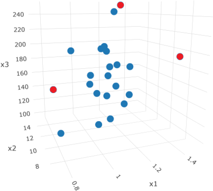
Johnson and Wichern [14] discuss the data set of public utility companies. The data is collected on 22 U.S. public utility companies for the year 1975. While Johnson and Wichern [14] use the data set for clustering variables 3-dimensional plots of the observations show presence of potential outliers. Eight variables are measured for each company: $X_{1}$ is income to debt ratio, $X_{2}$ is the rate of return on capital, $X_{3}$ is cost per KW, $X_{4}$ is annual load factor, $X_{5}$ is peak KW demand, $X6$ is sales, $X_{7}$ is percent nuclear and $X_{8}$ is the total fuel cost. Figure 1 shows the 3-dimensional plots of $X_{1}$ , $X_{2}$ and $X_{3}$ .

Figure 1.

Public Utility Data: Observations 5, 11 and 16 appear in red.

We use five methods of outlier detection, namely 1) ODD, 2) DB, 3) CHK, 4) MVE and 5) MCD to identify outliers of the data set.

•

The ODD method identifies observations 2, 5, and 16, which appears in color red in Fig. 1, as outliers.

•

The DB method with $d=1000$ identifies observations 5, 11, 16, and 19 as outliers.

•

The CHK method does not identify any outliers.

•

The MVE method identifies observations 5, and 11 as outliers.

•

The MCD method identifies observations 5, 8, and 11, 16 and 17 as outliers.

•

The LOF method identifies observations 2 and 5 as outliers.

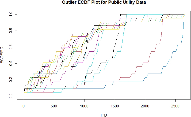
Modarres [20] considers a method of displaying multivariate data by a simultaneous plot of the empirical cumulative distribution functions (ECDFs) of the interpoint distances (IPDs). Figure 2 shows the ECDFs of the IPDs for 22 public utility observations. The three ECDFs on the far right of the Figure belong to the IPD of observations number 2, 5 and 16.

Figure 2.

Empirical CDFs of sample IPDs for Public Utility data. The ECDFs for observations 2 and 5 stands out on the far right in red and blue colors.

5.2 HDLSS colon cancer data

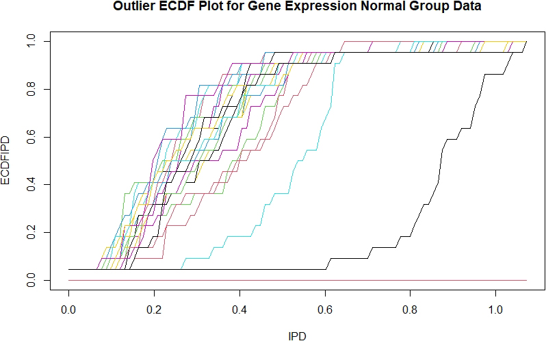
Alon, et al. [1] describe the colon tumor dataset containing the expression of the $p=2000$ genes across the 62 tissues. There are 22 normal and 40 cancer patients. We run the outlier detection techniques on this dataset. For the normal dataset, Odd finds one outlier at observation number (ON) 15, DB finds 3 outliers at $\textit{ON}=\{6,15,16\}$ , PC finds 7 outliers at $ON=\{1,2,4,7,10,13,18\}$ , CHK and LOF finds no outliers. In light of the simulation results, the findings by ODD and LOF are most credible.

Figure 3 shows the ECDFs of the IPDs for Gene Expression observations of 22 the patients in the cancer group. The ECDFs on the far right of the Figure belong to the IPD of observations number 15, which is detected by ODD. The ECDF of the next IPD belongs to observation 6, detected by LOF.

Figure 3.

Empirical CDFs of sample IPDs for normal Gene Expression data. The ECDFs for observations 5 and 15 stands out on the far right in blue and black colors.

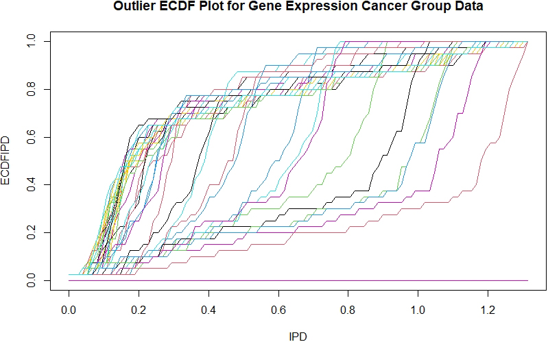
For the cancer cancer dataset, ODD fins no outlier, DB finds 4 outliers at $\textit{ON}=\{6,29,30,32\}$ , PC finds 5 outliers at $\textit{ON}=\{3,7,9,20,21\}$ }and CHK and LOF find no outliers. Figure 4 shows the ECDFs of the IPDs for 40 Gene Expression observations in the cancer group. The Figure does not show an ECDF on the far right that dominates the others. The findings by ODD, CHK and LOF are most credible.

Figure 4.

Empirical CDFs of sample IPDs for cancer Gene Expression data. No observation stands out as outlier as verified by ODD, CHK and LOF.

6. Summary and recommendations

The relationship between eigenvalues of the distance matrix and outliers is largely unknown. We show that outliers affect the pairwise distances and inflate the eigenvalues of the distance matrix. We obtain the eigenvalues of a constant distance matrix and the eigenvalues of a distance matrix that is affected by $k$ outliers. We show a discrepancy in the sizes of the eigenvalues of a distance matrix that is contaminated with outliers. We use this insight to offer a nonparametric test for outlier detection. Simulation experiments and analysis of public utility data set show that the proposed method performs much better than several competing methods. The distance matrix provides dimension reduction with $p>m$ . The new method searches for outliers through an $m\times m$ matrix of distances instead of an $m\times p$ matrix of observations. The $m\times m$ matrix of distances has smaller dimension and does not grow with $p$ . Our approach remains feasible with very large values of $p$ .

Affine equivariance of an outlier detection method requires it to produce the same results when the data changes due to linear transformations such as scaling, rotation and and translation (shifting). In other words, the method should still identify the same outliers before and after the transformation. Affine equivariance is important because it ensures that the method not affected by changes in the coordinate system or scaling of the data, making it more robust. While the ODD method is equivariant with respect to translation and rotation. It is not equivariant with respect to scaling. As noted earlier, it is common practice to standardize the dataset before searching for outliers.

A major advantage of the proposed method is lack of any tuning parameters. Other competing methods depend on specification of the radius of the neighborhood (DB), determining the lower and upper boundaries for location outlier detection (PC), the minimum number of the data points regarded as good points (MCD, MVE), a list containing the threshold values for each method (CHK), and the density threshold to identify core points for LOF. The ODD method is nonparametric since it does not make any distributional assumption. It also works for $p>m$ . Moreover, the ODD method detects marginal outliers and outliers in $q<p$ lower dimensions.

Footnotes

Acknowledgments

I would like to thank two anonymous referees for their constructive comments and suggestions.

References

Alon

Barkai

Notterman

D.A.

Gish

Ybarra

Mack

Levine

A.J.

, Broad patterns of gene expression revealed by clustering of tumor and normal colon tissues probed by oligonucleotide arrays, Proc Natl Acad Sci USA 96(1) (1999), 6745–6750.

Azzalini

Valle

A.D.

, The Multivariate Skew-normal Distribution, Biometrika 83(4) (1996), 715–726.

Azzalini

, The Skew-Normal and Related Distributions Such as the Skew-t, Package “sn”, (2020), http//azzalini.stat.unipd.it/SN.

Barnett

Lewis

, Outliers in Statistical Data, John Wiley & Sons, London, (1994).

Breunig

M.M.

Kriegel

H.P.

R.T.

Sander

, LOF: identifying density-based local outliers, In ACM Sigmod Record 29 (2000), 93–104.

Cabana

Lillo

R.E.

Laniado

, Multivariate outlier detection based on a robust Mahalanobis distance with shrinkage estimators, Statistical Papers 62(2) (2021), 1583–1609.

Filzmoser

Maronna

Werner

, Outlier identification in high dimensions, Computational Statistics and Data Analysis 52 (2008), 1694–1711.

Leva

Paganoni

A.M.

, Component-wise outlier detection methods for robustifying multivariate functional samples, Statistical Papers 61 (2020), 595–614.

Gower

J.C.

, Some distance properties of latent root and vector methods used in multivariate analysis, Biometrika 53(3) (1966), 325-338.

10.

Guo

Modarres

, Interpoint Distance Classification of High Dimensional Discrete Observations, International Statistical Review 87(2) (2019), 191–206.

11.

Hadi

A.S.

Imon

R.A.H.M.

Werner

, Detection of Outliers, Wiley Interdisciplinary Reviews: Computational Statistics 1(1) (2009), 57–70.

12.

Hahsler

Piekenbrock

Doran

, “dbscan” R package, https://cran.r-project.org/web/packages/dbscan/index.html, (2022).

13.

Hubert

Van der Veeken

, Outlier detection for skewed data, Journal of Chemometrics, Special Issue: Conferentia Chemometrica 22(3-4) (2007), 235–246.

14.

Johnson

R.A.

Wichern

D.W.

, Applied Multivariate Statistical Analysis, New Jersey: Prentice Hall (2007).

15.

Knorr

R.T.

, A Unified Approach for Mining Outliers, In Conf. of the Centre for Advanced Studies on Collaborative Research (CASCON), Toronto, Canada, (1997), 236–248, doi: 10.1145/782010.782021.

16.

Lüdecke

Ben-Shachar

M.S.

Patil

Waggoner

Makowski

, “performance”, An R package for assessment, comparison and testing of statistical models, Journal of Open Source Software 6(60) (2021), 31–39, doi: 10.21105/joss.03139.

17.

Madsen

J.H.

, “DDoutlier” R package, (2022), https://github.com/jhmadsen/DDoutlier.

18.

Mahalanobis

P.C.

, On the Generalised Distance in statistics, Proceedings of the National Institute of Sciences of India 2 (1936), 49–55.

19.

Mardia

K.V.

Kent

J.T.

Bibby

J.M.

, Multivariate Analysis. Academic Press, London, (1979).

20.

Modarres

, Graphical Comparison of High Dimensional Distributions, International Statistical Review 88(3) (2020), 698–714.

21.

Modarres

Song

, Interpoint Distances: Applications, Properties and Visualization, Applied Stochastic Models in Business and Industry 36(6) (2020), 1147–1168.

22.

Modarres

, Outlier Tests of High Dimensional Observations, Journal of nonparametric Statistics 34 (2022), 206–227.

23.

Modarres

, A High Dimensional Dissimilarity Measure, Computational Statistics and Data Analysis, (2022), doi: 10.1016/j.csda.2022.107560.

24.

Peña

Prieto

, Multivariate Outlier Detection and Robust Covariance Matrix Estimation, Technometrics 43(3) (2001), 286–310.

25.

Rousseeuw

P.J.

, Multivariate Estimation with High Breakdown Point, In: Grossmann

Pflug

Vincze

Wertz

, eds, Mathematical Statistics and Applications, Volume B. Dordrecht: Reidel Publishing Company, 1985, pp. 283–297.

26.

Rousseeuw

P.J.

van Driessen

, A fast algorithm for the minimum covariance determinant estimator, Technometrics 41 (1999), 212–223.

27.

Shurygin

A.M.

, Using interpoint distances for pattern recognition, Pattern Recognition and Image Analysis 16(4) (2006), 726–729.

Using eigenvalues of distance matrices for outlier detection

Abstract

Keywords

1. Introduction

2. Distance matrix

.

.

.

4.2 Multivariate normal and t 15 samples

Table 2 Normal data: The proportion of times outliers are detected when there are NOUT outliers in 1000 experiments, m = 25 and each outlier is shifted by 3 units

Table 4 Skew-normal data: The proportion of times outliers are detected when there are NOUT outliers in 1000 experiments, m = 25 and each outlier is shifted by 3 units

Table 6 Absolute normal data: The proportion of times outliers are detected when there are NOUT outliers in 1000 experiments, m = 25 and each outlier is shifted by 3 units

Table 7 Normal data with p > m : The proportion of times outliers are detected when there are NOUT outliers in 1000 experiments, m = 25 , p = 100 and each outlier is shifted by 3 units

5.1 Public utility data

Footnotes

Acknowledgments

References

4.2 Multivariate normal and $t_{15}$ samples

Table 2
Normal data: The proportion of times outliers are detected when there are NOUT outliers in 1000 experiments, $m=25$ and each outlier is shifted by 3 units

Table 4
Skew-normal data: The proportion of times outliers are detected when there are NOUT outliers in 1000 experiments, $m=25$ and each outlier is shifted by 3 units

Table 6
Absolute normal data: The proportion of times outliers are detected when there are NOUT outliers in 1000 experiments, $m=25$ and each outlier is shifted by 3 units

Table 7
Normal data with $p>m$ : The proportion of times outliers are detected when there are NOUT outliers in 1000 experiments, $m=25$ , $p=100$ and each outlier is shifted by 3 units