A bitemporal RDF index based on skip list

Abstract

The Resource Description Framework (RDF) is a framework for expressing information about resources in the form of triples (subject, predicate, object). The information represented by the standard RDF is static, $i . e .$ , that does not change over time. To better deal with a large amount of time-related information, temporal RDF is proposed. Consequently, how to explore index technology to efficiently query temporal information has become an important research issue, but the research on the index of temporal RDF is still short, especially the index of bitemporal RDF. Bitemporal RDF can represent more complicated situations (e.g., RDF triples with both valid time and transaction time). Indexes for bitemporal RDF can further expand the application scenarios and functions of temporal RDF. In this paper, we propose an efficient index for bitemporal RDF queries. The index innovatively introduces and re-designs skip list structure into the bitemporal RDF query. We also investigate how to cover almost all query patterns with as few indexes as possible. In addition, although the proposed index is conceived for temporal RDF, it also takes into account the performance of standard RDF queries when the time element is unknown. Finally, we run experiments with synthetic data sets of different sizes using the Lehigh University Benchmark (LUBM), and results prove that the proposed index is scalable and effective.

Keywords

Resource Description Framework (RDF)temporal RDF bitemporal RDF index

1. Introduction

In recent years, the number of publicly available valuable resources on the Web has increased. Getting insight into data and extracting knowledge from huge repositories of information has become a critical task [1]. The Resource Description Framework (RDF) [2] is a popular framework for expressing information about resources and their semantics in the form of triples (subject, predicate, object), also abbreviated as ( $s$ , $p$ , $o$ ). In particular, time information is an important and inevitable part in almost any Web application [3]. However, the information represented by the standard RDF is static, $i . e .,$ that does not change over time or the whole RDF dataset corresponds to a particular time point [4]. To better deal with time-related information, temporal RDF [5] is proposed. The basic form of temporal RDF is to use temporal labels to annotate RDF triples or RDF triple elements (see [6] in detail). The most frequently occurring time types are valid time and transaction time [7, 8, 9, 10, 11]. The valid time records the time when the data is true in reality. The transaction time records the time when the data is recorded in the database.

The popularity of RDF in real-world applications ( $e . g .$ , the Linked Open Data (LOD) cloud, knowledge graphs, and the Semantic Web) drives the development of RDF storage, query, and indexing [1]. Some work is devoted to the index of RDF, including the k2-trees based BMatrix index [1] and the graph based GRIN index [12] (please refer to the related work of Section 2 for more detail). In recent years, with the wide application of RDF in time data management, how to explore index technology to efficiently query temporal RDF information has gradually received considerable attention. However, the research on the index of temporal RDF is still short, especially the research on bitemporal RDF index.

The bitemporal RDF can represent more complicated situations ( $e . g .$ , the RDF triples with both valid time and transaction time). Such cases often occur in many practical applications, and thus some relatively complex query requirements are raised. For example, a user would like to query the names of all schools that Bob has attended and the time spent in each school from the records of the past five years, where “the time spent in each school” denotes the valid time that Bob actually attended the school, while “the records of the past five years” denotes the transaction time that the data is recorded during the past five years. Therefore, index for bitemporal RDF is very necessary and useful for improving query efficiency, and also can further expand the application scenarios and functions of temporal RDF.

In this paper we propose an efficient index for bitemporal RDF query. The main contributions can be summarized as follows:

We propose an efficient index for bitemporal RDF query. The index innovatively introduces and re-designs the skip list structure (which is a data structure equivalent to a balanced tree in probability [13]) into the bitemporal RDF query.

We also investigate how to cover almost all query patterns with as few indexes as possible.

Moreover, although the proposed index is conceived for temporal RDF, the index also takes into account the performance of standard RDF queries when the time element is unknown.

Finally, we run experiments with synthetic data sets of different sizes using the Lehigh University Benchmark (LUBM), and results prove that the proposed index is scalable and effective.

The remainder of this paper is organized as follows. Section 2 presents a brief overview of related work in classical RDF index and temporal RDF index. Section 3 proposes our scheme about bitemporal RDF index. Section 4 further gives the index construction and maintenance algorithms. Section 5 is the experimental evaluation of our approach. Section 6 concludes this paper and sketches our future work.

2. Related work

In this section, we briefly review the related work on indexing RDF data and temporal RDF data. RDF or temporal RDF data are usually stored in the form of RDF graphs or tables [6, 14]. Therefore, the indexing methods can also be roughly divided into graph indexing methods and table indexing methods.

2.1 RDF index

RDF-3X is a RISC-style Engine for RDF [15]. RDF-3X builds indexes on all 6 permutations of the three dimensions that make up the RDF triples. It also builds indexes on the count aggregation variants of all two-dimensional and all one-dimensional projections. Each of these indexes can be compressed very well, and the total storage space for all indexes together is less than the size of the primary data.

Madduri and Wu [16] propose a new strategy based on bitmap index which contains three composite indexes each with two columns as keys. The keys are composite values of predicate-subject, predicate-object, and subject-object. Utilizing the constructed bitmap indexes can accelerate SPARQL query evaluation.

Recent works have proposed methods to reduce the redundancy in the index permutations. In particular, RDFCSA [17] uses a compact suffix-array (CSA) in which one permutation suffice can efficiently support all triple patterns. Triples can be indexed cyclically in a CSA, that is to say, in a ( $s$ , $p$ , $o$ ) permutation, one can continue from $o$ back to $s$ , so the permutations of ( $s$ , $p$ , $o$ ), ( $p$ , $o$ , $s$ ) and ( $o$ , $s$ , $p$ ) are covered in one CSA index. The BMatrix [1] is also an RDF index based on k2-trees, and it is especially suitable for the datasets with a relatively large number of predicates.

GRIN [12] is a graph based RDF index. GRIN divides the graph hierarchically into regions based on the distance of its nodes to selected centroids. These regions will eventually form a tree. The root element chooses a node and distance such that all nodes of the graph are covered. GRIN has been extended to tGRIN [18] to handle temporal RDF queries, as it will be introduced in Section 2.2.

2.2 Temporal RDF index

The research on the index of temporal RDF is still short. Several works only consider the index of temporal RDF with a single time dimension, $e . g .$ , only for the valid time or only for the transaction time. So far, to our best knowledge, there is no report on bitemporal RDF index.

tGRIN [18] is an index structure based on GRIN [12] to process RDF valid time annotations. The tGRIN index structure is a tree whose root implicitly represents the entire space. Since the presence of temporal annotations on the triples, tGRIN changes the semantics of queries and distance measures in the tRDF graph. Another difference with GRIN is that tGRIN builds an $n$ -ary tree instead of a binary tree, so the index construction method will be different. Another keyTree index structure of RDF graphs for processing valid time is proposed in [19]. First, it stores the temporal RDF graph in the form of an adjacency table and adopts breadth-first traversal to find some paths of the graph. Then it obtains the prefix paths and suffix paths in the graphs and establishes the prefix, path index and suffix index, respectively.

An index for transaction time is proposed in [20]. The index contains two levels: the first one is a global index for time information of RDF triples and the second one is a local index for non-time information of RDF triples. The global index is a temporal K-D tree and the local index use composition bitmap to index.

3. Bitemporal RDF index

In this section, we first briefly introduce the basic notations of bitemporal RDF in Section 3.1. Then, in Section 3.2 we make some preparation process before we build the indexing for bitemporal RDF. Finally, we propose our bitemporal RDF index structure in Section 3.3.

3.1 Bitemporal RDF

An RDF dataset consists of (subject, predicate, object) triples, abbreviated as ( $s$ , $p$ , $o$ ). The information described by RDF is static and cannot represent changes over time. For representing and handling temporal information, the temporal RDF was proposed. The basic idea of temporal RDF is to use temporal labels to annotate RDF triples or RDF triple elements [20]. The two main types of time dimensions are valid time and transaction time [7]. Valid time represents the time when the data is true in reality. Transaction time represents the time when the data is recorded in the database. In the database, the expressions of valid time and transaction time are not clearly defined, and they can be time points, time intervals, or a collection of gradually constant time points. According to the characteristics of the transaction time, when the data is recorded in the database, the current time becomes the beginning of the transaction time of this data. Since the time when the data is deleted cannot be determined and most of the data marked with temporal information will not be deleted, the end of the transaction time is open. Therefore, use the time interval to represent the valid time, and the time point to represent the transaction time. However, most of the previous work only considered the valid time or the transaction time separately [6]. In this paper, we consider these two types at the same time (i.e., bitemporal RDF). In brief, we use [ts, te] to represent the time interval of valid time, ts represents the start time, and te represents the end time. For transaction time, we use [ $t$ ] to indicate the time point.

Definition 1. A bitemporal RDF triple is an RDF triple annotated by two temporal labels, valid time and transaction time. The representation of a bitemporal RDF triple is ( $s$ , $p$ , $o$ ): [ts, te][ $t$ ], where:

$s$ , $p$ , $o$ represent the subject, predicate and object in RDF triples, respectively.

[ts, te] represents the valid time of the RDF triple, which starts from the time point ts to the end of the time point te. When ts $=$ te indicates that the valid time of the triple is a time point.

[ $t$ ] represents the transaction time of the RDF triple. It represents the time when the triplet was inserted into the database.

Table 1
An example of bitemporal RDF data set

$s$	$p$	$o$	Valid time	Transaction time
Bob	Member of	Primary school	2004.8–2010.7	2010.7
Bob	Member of	High school	2010.8–2016.7	2016.9
Bob	Member of	University	2016.8–2020.7	2021.1
Alice	Position	Staff	2012.7–2014.12	2015.1
Alice	Position	Manager	2016.8–2020.7	2021.7
Tom	Lives in	London	2004.8–2010.7	2010.7
Tom	Lives in	Leeds	2010.8–2016.7	2016.9

The bitemporal RDF triples constitute a bitemporal RDF data set. Table 1 shows a simple example of bitemporal RDF data set.

Bitemporal RDF triples that have both valid time and transaction time can represent more complicated situations, which often occur in many practical applications, and thus some relatively complex query requirements are raised. For example, a user would like to query the names of all schools that Bob has attended and the time spent in each school from the records of the past five years, where “the time spent in each school” denotes the valid time that Bob actually attended the school, while “the records of the past five years” denotes the transaction time that the data is recorded during the past five years. However, neither the standard RDF nor the previous temporal RDF can support this kind of queries. Therefore, an index for bitemporal RDF is necessary and useful for further expanding the application scenarios and functions of temporal RDF.

3.2 Preparation before indexing

Figure 1.

An example of transforming the bitemporal RDF data set into tuples of integer IDs.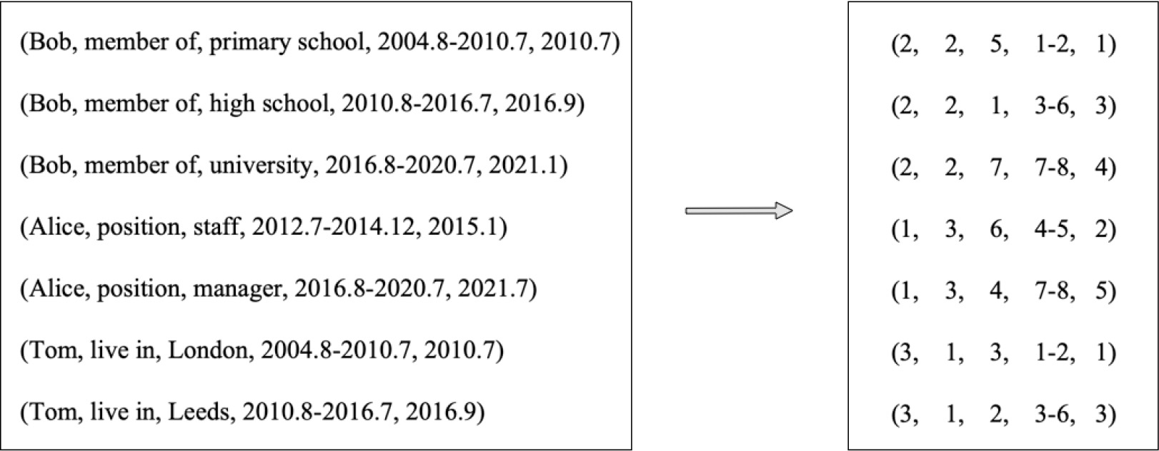

The queries of bitemporal RDF triples are more complicated. For standard RDF, if letting $s$ , $p$ , $o$ denote RDF value terms and s, p, o variables, there are six triple patterns: (s, $p$ , $o$ ), ( $s$ , p, $o$ ), ( $s$ , $p$ , o), (s, p, $o$ ), ( $s$ , p, o) and (s, $p$ , o). For bitemporal RDF, there are five elements in the tuple as shown in Definition 1. Each element of the tuple is either a value or a variable. Therefore, there are a total of 2*2*2*2*2 $=$ 32 combination modes. Removing the two special cases that are all variables or all values, we can find that there are thirty query situations in bitemporal RDF, which is 5 times that of standard RDF. To reduce the memory occupied by the index, we respectively encode the subject, predicate, object, and two time types as integer IDs, which can significantly reduce the memory occupied by the index. On this basis, the bitemporal RDF ( $s$ , $p$ , $o$ ): [ts, te][ $t$ ] can be expressed as a tuple of integer IDs as shown in Fig. 1.

3.3 Index structure

In this section we propose our bitemporal RDF index structure. We first introduce the motivation and ideas of our index. Then, we propose the detailed structure of the index.

3.3.1 Motivation and ideas of index

Our index innovatively introduces and re-designs the skip list structure into the bitemporal RDF query. A skip list [13] is a data structure that is probabilistically equivalent to a balanced tree. For many applications, a skip list is a more natural representation than a tree and leads to simpler algorithms. A skip list is a sorted multi-level linked list, where higher-level elements are a subset of lower-level elements. The search starts from the sparsest and highest level until the element to be searched is between two elements in this level, then it goes to the next level and repeats the search until the searched element is found.

The skip list is selected as the main structure of our bitemporal RDF index for the following reasons. First of all, the time complexity of skip list query is O(logn), the query efficiency is high and stable, and the update time complexity is relatively low, which is convenient for index maintenance and update. Secondly, the skip list is developed on the basis of the linked list structure. Compared with the tree structure, the linked list structure is often a more natural representation of data. Finally, the skip list is an ordered data structure. The query for temporal information will involve many comparison operations. The order of the skip list can well support the comparison query. Therefore, the skip list is used as the main structure for indexing bitemporal RDF data.

Moreover, as mentioned in Definition 1, RDF data adds two time dimension labels, valid time and transaction time, and thus triples become five-tuples. In this case, basic query patterns may grow exponentially, and the constructed index needs to cover more query patterns. At the same time, temporal information and RDF information are two completely different types of information, and an index structure suitable for RDF may not be suitable for temporal information, and vice versa. Therefore, when designing a bitemporal RDF index, in addition to considering the query efficiency and the occupied space, the compatibility of the index structure needs to be considered, and it needs to be applicable to both RDF data and time data.

For bitemporal RDF query, the following query patterns may appear:

No temporal information is involved in the query, only conditions of subject, predicate and object are constrained. In this case the query is the same as standard RDF.

Temporal information is used as a constant in the query. At this point, the query result needs to meet the requirements for temporal information while satisfying the triple conditions.

Temporal information is used as a variable in the query, and the temporal information of one or more triples needs to be obtained as the query result.

Figure 2.

The structure of the VT-Index.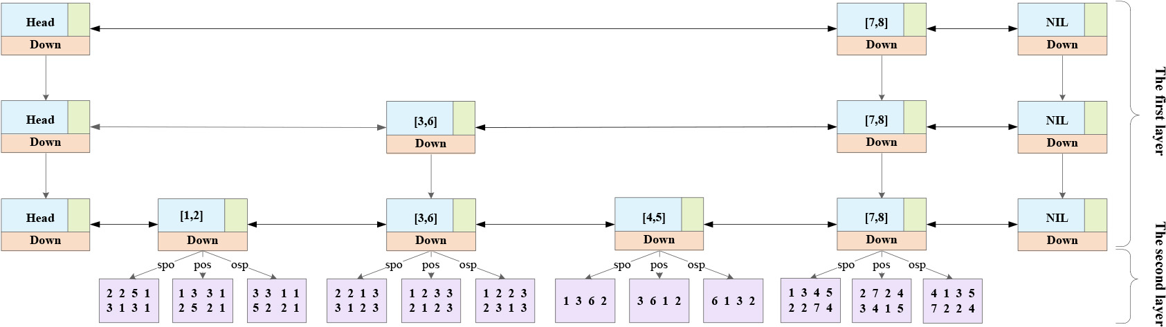

The temporal information mentioned above refers to valid time and/or transaction time. Building an index against bitemporal RDF requires taking care of the query patterns described above. Therefore, we propose a two-layer index structure based on skip list to index bitemporal RDF data. The first layer is a skip list structure including multi-level linked lists, and the second layer is the data storage layer (see Fig. 2 for an example). Depending on whether the query condition includes temporal information, the information contained in each layer is also different.

When the temporal information is not involved in the query or the temporal information is the variable (i.e., the target of the query), we need to filter and search the data from the RDF triple data. The first layer of the index stores the RDF triple data, that is, the skip list is used to group and filter the RDF triple data. After preliminary filtering, the remaining information is stored in the second layer of the index to continue comparison and search.

When the temporal information appears as a constant constraint in the query, the temporal information can be used to index the data. The first layer of the index is the temporal information, and the data is grouped according to the temporal information. The data with the same temporal information is divided into the same node of the skip list. Continue to search in the nodes that meet the query conditions. At the same time, comparison operations such as greater than and less than are often required for temporal information, so the skip list structure of the index temporal information is processed from a single-way linked list to a doubly-linked list to better support bidirectional search.

3.3.2 Index structure

For a more specific description, we first take the valid time as the first layer of the index as an example, which we call VT-index. The constructing of the VT-index can be divided into the following steps. First, collect all the valid time intervals in the data set and construct a skip list on the valid time intervals. Each time interval corresponds to a node in the skip list, and thus the valid time can be indexed through them. Further, in order to store the other elements ( $i . e .$ , $s$ , $p$ , $o$ and $t$ ) in the bitemporal RDF tuples of Definition 1, the structure of skip lists is expanded. Considering that there may be different query patterns when the valid time as query condition, three arrays are added to each node to store the other elements in a different order. Then, all bitemporal RDF data with the same valid time interval is put in its corresponding node in the skip lists. At the same time, when the size of the data set is large, the amount of data under the same valid time is still a lot. To query other elements more efficiently and ensure that the data in the node is in order so that binary search can be used, the tuples with the same valid time are sorted in the order of ( $s$ , $p$ , $o$ , $t$ ), ( $p$ , $o$ , $s$ , $t$ ), and ( $o$ , $s$ , $p$ , $t$ ). In this way, the RDF basic query patterns can be covered completely after determining the valid time. In detail, the structure of the index for the valid time (VT-index) of Fig. 1 is shown in Fig. 2.

Based on the index in Fig. 2, the one-way pointer of the skip list is changed to a two-way pointer, which can search in two directions. It can better support interval query and comparison query of temporal information. At the same time, the different sorting sequences can be selected according to the corresponding known conditions. For example, if the valid time, the subject and the predicate are known (i.e., querying the object and transaction time), or the valid time and the subject are known (i.e., querying the predicate, object and transaction time), after finding the corresponding valid time in the skip lists, the query will be able to enter the sequence of ( $s$ , $p$ , $o$ , $t$ ) for binary search and quickly find the corresponding object and transaction time or the corresponding predicate, object and transaction time.

Figure 3.

The structure of the TT-Index.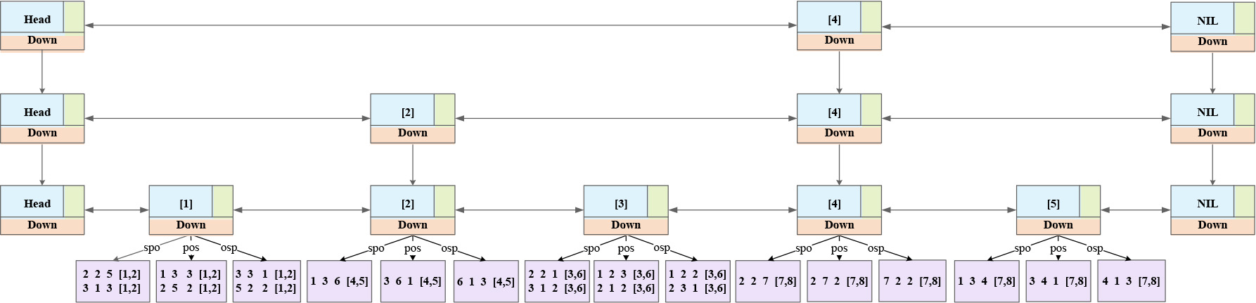

The indexing which transaction time [ $t$ ] is in the first layer is similar to the VT-index, the difference is that the transaction time is a timestamp instead of a time interval. The order of the data under the same transaction time in the skip list node is ( $s$ , $p$ , $o$ , [ts, te]), ( $p$ , $o$ , $s$ , [ts, te]) and ( $o$ , $s$ , $p$ , [ts, te]). Figure 3 shows the structure of the transaction time as the first layer of the index (i.e., TT-index).

In addition, when the temporal information is not involved in the query or the temporal information is the variable (i.e., the target of the query), the index needs to filter data with triplet data. At this time, temporal data cannot be used as the first layer of the index. Next, take the index with the subject as the first layer as an example, that is, S-index. Describe the structure of the index when triple data is used as the query entry. (analogous for the predicate and the object, i.e., P-index and O-index). First, create a skip list for all subject IDs, then group the triples according to the subject and put the triples with the same subject together. Further, to store the remaining elements of the bitemporal RDF tuple in the skip list, the skip list needs to be expanded. But unlike the expanding methods for the VT-index and the TT-index above, the S-index only needs one storage structure and is arranged in the order of ( $p$ , $o$ , [ts, te], [ $t$ ]). Figure 4 shows the structure of the S-index in Fig. 1.

It should be noted that there are two hyper-parameters of skip list that need to be set: one is the MaxLevel, and the other is a fraction $p$ . If $p$ is not set, we will have a probability distribution where half of the nodes that have level $i$ pointers also have level $i+$ 1 pointers. For MaxLevel we choose MaxLevel $=$ log ${}_{1/p}N$ , where $N$ is an upper bound on the number of elements in a skip list. The first node of skip lists is a special node called Head, as shown in Figs 1–4. The Head of a list has forward pointers at levels 1 through MaxLevel. Use a NIL key at the end of the list to represent a key greater than any legal key. All levels of all skip lists are terminated with NIL. A new list is initialized so that the level of the list is equal to 1 and all forward pointers of the list’s header point to NIL [12]. We set $p$ to 1/2 and the MaxLevel according to the value of $p$ and the size of the largest data set.

Table 2

Matching of index and query patterns

Query pattern	Matchable index
(s,?p,?o,?vt,?tt), (s,p,?o,?vt,?tt)	S-index
(?s,p,?o,?vt,?tt), (?s,p,o,?vt,?tt)	P-index
(?s,?p,o,?vt,?tt), (s,?p,o,?vt,?tt)	O-index
(s,?p,?o,vt,?tt), (s,p,?o,vt,?tt)	VT-index, S-index
(?s,p,?o,vt,?tt), (?s,p,o,vt,?tt)	VT-index, P-index
(?s,?p,o,vt,?tt), (s,?p,o,vt,?tt)	VT-index, O-index
(s,?p,?o,?vt,tt), (s,p,?o,?vt,tt)	TT-index, S-index
(?s,p,?o,?vt,tt), (?s,p,o,?vt,tt)	TT-index, P-index
(?s,?p,o,?vt,tt), (s,?p,o,?vt,tt)	TT-index, O-index
(s,?p,?o,vt,tt), (s,p,?o,vt,tt)	VT-index, TT-index, S-index
(?s,p,?o,vt,tt), (?s,p,o,vt,tt)	VT-index, TT-index, P-index
(?s,?p,o,vt,tt), (s,?p,o,vt,tt)	VT-index, TT-index, P-index
(s,p,o,?vt,?tt)	S-index, P-index, O-index

Figure 4.

The structure of the S-Index.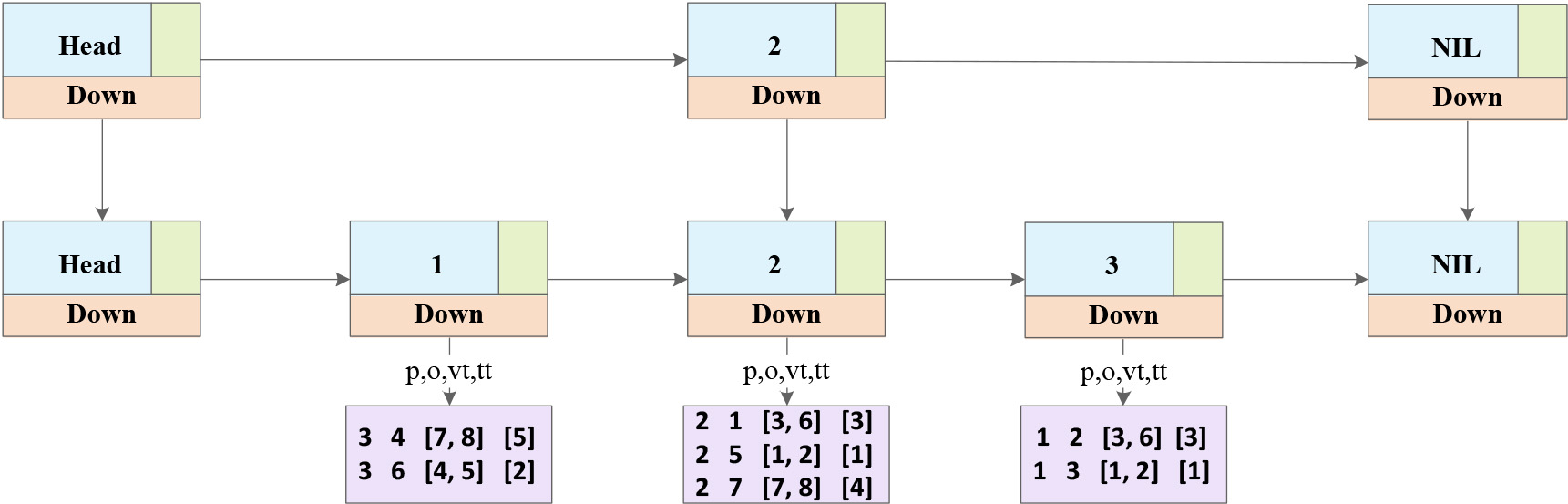

In summary, the designed index is a two-layer index. In order to fully cover the basic query mode, corresponding indexes are established for different situations. Given a query, according to the given conditions, different query modes are matched to select the appropriate index to search for the results. The specific matching scheme is shown in Table 2. In the table, $s$ , $p$ , $o$ , vt, and tt are used to represent the subject, predicate, object, valid time and transaction time respectively. A mark “?” in front indicates that the value is an unknown variable at this time.

As can be seen from Table 2, some query patterns can match more than one index. In the real-world applications, because this query mode can match multiple indexes, we should choose the one with the lower query cost. For example, ( $s$ , ? $p$ , ? $o$ , vt, ?tt) can select both S-index and VT-index. A guideline for using indexes is that we should try to use as discriminative information as possible. That is, it depends on whether there is less data divided under the same subject in the data set (where S-index will be chosen) or less data divided under the same valid time (where VT-index will be chosen).

4. Index construction and maintenance

On the basis of the bitemporal RDF index proposed in Section 3, in this section we further give the index construction and maintenance algorithms. We first process the data set to get the integer IDs of subject, predicate, object, valid time and transaction time respectively. Then, the bitemporal RDF index is constructed and stored in memory, which will be used for querying. Moreover, when the temporal RDF data changes, the index will be accordingly maintained, including addition, deletion and modification.

4.1 Data processing

The purpose of data processing is to transform the RDF string data into the integer ID representation. On one hand, as shown in Fig. 1 and mentioned in Section 3.2, the integer ID representation of the RDF string data can reduce the space occupied by the index and speed up processing. On the other hand, because a skip list is an ordered data structure, the integer ID representation can also be easily processed into an order form, which is convenient for building subsequent index.

Table 3
Data processing algorithm

Algorithm Data processing algorithm
Input: Data Set D
Output: S. // array of integer IDs for subjects
1.	$\text{S}\leftarrow[]$
2.	for data in D do
3.	s $\leftarrow$ split (D) // split data
4.	listS.add(s)
5.	if s not in setS then
6.	setS.add(s)
7.	endif
8.	endfor
9.	sort (setS) // sort the setS
10.	S $\leftarrow$ convert (listS, setS) // use lists and sorted sets to get S
11.	return S

Here we take the algorithm for processing subject data as an example, and the specific process is shown in Table 3.

As shown in Table 3, the data processing algorithm first loads the data set into memory, and splits and obtains values of the subjects (Lines 1–3). After that, the values of the subjects are added into a list. Moreover, a set variable is created to store the values of all subjects and guarantee that each subject occurs only once (Lines 4–8). Next, the set is sorted in the order of characters (Line 9). Finally, the subjects in the list are traversed, and the position of the value of a subject in the sorted set is represented as an integer of the subject (Line 10). Now, we obtain the integer ID representation of the subjects.

4.2 Index construction

As introduced in Section 3, the S-index, P-index, and O-index have similar structures, and they all use an element in a triple as the first layer of the index. The second layer of the index is the rest elements of the triple, which is stored in different orders for better matching different query modes. Here we take S-index as an example to introduce the index build algorithm.

Table 4
Triple index build algorithm

Algorithm Triple index build algorithm
Input: $\text{S},\text{P},\text{O},\text{VT},\text{TT}$ // arrays of integer representation of data
Output: S-Index // target index
1.	S-Index $\leftarrow$ createSkipList()
2.	S-Index.init() // create skip list and initialize it
3.	for s in S do
4.	S-Index.insert(s) // insert the data in S into the skip lsit
5.	end for
6.	sortData(S,P,O,VT,TT) // sort data by SPO query mode
7.	for i $=$ 1 $\to$ m do
8.	add(S[i],P[i],O[i],VT[i],TT[i]) // add the sorted data to the skip list
9.	end for
10.	return S-Index
11.	add(s,p,o,vt,tt)
12.	head $\leftarrow$ S-Index.head, tail $\leftarrow$ S-Index.tail // get head and tail nodes of skip list
13.	for i $=$ L $-$ 1 $\to$ 0 do // L represents the maximum number of layers of skip list
14.	while head.next[i]! $=$ tail & head.next[i].value $<$ s do
15.	head $=$ head.next[i] // find the first node smaller than the current data from
	top to bottom
16.	end while
17.	end for
18.	head $=$ head.next[0]
19.	head.set(p,o,vt,tt) // add data to the corresponding node

As shown in Table 4, a skip list is first created, and the data stored in the array $S$ in Table 3 (i.e., the integer IDs of the subjects in triples) is inserted into the skip list (Lines 1–5). Then, the predicates and objects in triples will be sorted and added into the skip list (Lines 6–18). Since this index in Table 4 is primarily constructed based on the subjects, the rest of the data in triples will be sorted by subjects (i.e., in the order of spo) (Line 6). In order to add the sorted data into the skip list, the first step is to get head and tail nodes of the skip list (Line 11). The second step is to start from the head node of the skip list, find the first node smaller than the current inserted data by searching from the upper layer to the lower layer, and then insert the current inserted data after this node (Lines 12–17). The algorithm finally returns the constructed S-index.

Table 5

Temporal index build algorithm

Algorithm Temporal index build algorithm
Input: S, P, O, VT, TT // arrays of integer representation of data
Output: VT-index // target index
1.	VT-index $\leftarrow$ createSkipList()
2.	VT-index.init() // create skip list and initialize it
3.	for vt in VT do
4.	VT-index.insert(vt) // insert the data in VT into the skip Isit
5.	end for
6.	sortData(S,P,O,VT,TT) // sort data by spo query mode
7.	for i $=$ 1 $\to$ m do
8.	add(VT[i],S[i],P[i],O[i],TT[i]) // add the sorted data to the skip list
9.	end for
10.	sortData(P,O,S,VT,TT) // sort data by pos query mode
11.	for i $=$ 1 $\to$ m do
12.	add(VT[i],S[i],P[i],O[i],TT[i])
13.	end for
14.	sortData(O,S,P,VT,TT) // sort data by osp query mode
15.	for i $=$ 1 $\to$ m do
16.	add(VT[i],S[i],P[i],O[i],TT[i])
17.	end for
18.	return VT-index
19.	add(vt,s,p,o,tt){
20.	head $\leftarrow$ VT-index.head, tail $\leftarrow$ VT-index.tail // get the head and tail nodes of the skip list
21.	for i $=$ L $-$ 1 $\to$ 0 do
22.	while head.next[i]! $=$ tail& head.next[i].value $<$ vt do
23.	head $=$ head.next[i]
24.	end while
25.	end for
26.	head $=$ head.next[0]
27.	head.set(s,p,o,tt) // add data to the corresponding node

Then, we give an algorithm of constructing index in which the temporal information is the first layer. When the temporal information is shown in the query, the data can be filtered and queried using the temporal information. The algorithms for constructing the VT-index and the TT-index are similar, and here we take the algorithm of constructing the VT-index as an example, as shown in Table 5.

Table 5 shows the algorithm for constructing the VT-index. First, a skip list is created, and the temporal information is inserted into the skip list and becomes the first layer of the index (Lines 1–5). Since this index in Table 5 is primarily constructed based on the temporal information, In order to cover more query patterns the triple data needs to be stored in spo, pos and osp modes. Therefore, these data needs to be sorted according to the three modes, and then add the sorted data into the second layer of the index (Lines 6–17). The adding process (Lines 19–27) is similar to the process in Table 4. The algorithm finally returns the constructed temporal index.

4.3 Index maintenance

Temporal RDF data may be updated frequently due to the addition of temporal information. When the data updates, the index needs to be changed accordingly. Therefore, the update efficiency of the index is also very important. Using the skip list as the main structure of the index does not need to split and redistribute nodes like a tree structure when updating. It only needs to modify the front and back pointers of the corresponding nodes and the high-level pointers. Index maintenance mainly refers to addition, deletion and modification.

Table 6
Index addition algorithm

Algorithm Index addition algorithm
Input: VT-index, s, p, o, vt, tt // original index, target data to be added
Output: VT-index // updated index
1.	head $\leftarrow$ VT-index.head,tail $\leftarrow$ VT-index.tail
2.	for i $=$ L $-$ 1 $\to$ 0 do
3.	while head.next[i]! $=$ tail& head.next[i].value $<$ vt do
4.	head $=$ head.next[i] // find the predecessor node of the target data
5.	end while
6.	end for
7.	prev $=$ head // record the predecessor node
8.	head $=$ head.next[0]
9.	if head.value $==$ vt then // insert data into the second layer if the corresponding value exists
10.	head.set(s,p,o,tt)
11.	else // insert if the corresponding value docs not exist
12.	newNode $\leftarrow$ Node( s,p,o,vt,tt ) // create a new node
13.	newNode.next = prev.next,prev.next $=$ newNode // insert a node into the
	data chain
14.	if randomLevel $>$ L then // if the randomly generated layer number is greater
	than the current highest layer number
15.	L $=$ L $+$ 1 // update the number of layers of the skip list
16.	endif
17.	endif
18.	return VT-index

In general, the operations for updating different indexes are similar. For a more concise and clear description, we use VT-index as an example to illustrate. Table 6 shows the algorithm of adding data to the VT-index.

To add data to an index as shown in Table 6, we first need to obtain the head and tail nodes of the index (Line 1). Afterwards, find the first node smaller than the current inserted data by searching from the upper layer to the lower layer, we call it the predecessor node of the current node. The predecessor node is recorded (Lines 2–7). Compare whether the data of the next node of the previous node is equal to the target data, and if the value of the node to be inserted exists in the skip list, insert data into the second layer of the index to complete the addition of data (Lines 8–10). Otherwise insert operations at each level of the index are performed by creating a new node, storing data in the new node, and inserting the new node into the index (Lines 11–13). Because the first layer structure is a skip table structure, when inserting nodes into the skip table, it is necessary to consider whether to update the maximum number of layers of the skip table. The solution we adopt is to randomly generate an integer as random level after inserting a node. If the generated random level is greater than the current maximum level of the skip list, add the value of the current level of the skip list by one (Lines 14–16).

Table 7

Index modification algorithm

Algorithm Index modification algorithm
Input: VT-index vt₁, s₁, p₁, o₁, tt₁, s, p, o, tt //original index, original data, modified data
Output: VT-index // updated index
1.	head $\leftarrow$ VT-index.head,tail $\leftarrow$ VT-index.tail
2.	for i $=$ L $-$ 1 $\to$ 0 do
3.	while head.next[i]! $=$ tail& head.next[i].value $<$ vt do
4.	head $=$ head.next[i] // find the predecessor node of the old data
5.	endwhile
6.	end for
7.	head $=$ head.next[0]
8.	if head.value! $=$ vt then // if the target value does not exist
9.	return false
10.	else // if the target value is found, modify it
11.	head.findSPO(s₁, p₁).set(o,tt)
12.	head.findPOS(p₁, o₁).set(s,tt)
13.	head.findOSP(o₁, s₁).set(p,tt)
14.	endif
15.	return VT-index

The algorithm for modifying the index is shown in Table 7.

As shown in Table 7, to modify the index, we need to provide the original data and the target data to be modified. When modifying, first find the location of the original data in the index, and then modify it to new data. In VT-index, we find the original data from the valid time as the search entry. Specifically, first find the valid time in the original data in the VT-index (Lines 1–7). If the valid time in the original data cannot be found in the first layer of the VT-index, it means that the data is wrong, and it can be returned directly (Lines 8–9). If the valid time in the original data is found in the first layer of the VT-index, the remaining data is modified to the target value in the second layer of the VT-index (Lines 10–14). It should be noted that the modification algorithm introduced here does not modify the first layer of the index, but only modifies the second layer data in the index. If the first layer of the index also needs to be modified, the method we adopt is to delete the original data as will be introduced in the following and then add the modified data.

Table 8

Index deletion algorithm

Algorithm Index deletion algorithm
Input: S-index, s, p, o, vt, tt // original index, target data to be deleted
Output: S// index after deleting the target data
1.	head $\leftarrow$ S-index.head
2.	fori $=$ L $-$ 1 $\to$ 0 do
3.	while head.next[i]! $=$ tail& head.next[i].value $<$ s do
4.	head $=$ head.next[i] // find the predecessor node of the data to be deleted
5.	endwhile
6.	end for
7.	head $=$ head.next[0]
8.	if head.value! $=$ s then // returns if the value to be deleted does not exist
9.	return false
10.	else
11.	head.delete(p,o,vt,tt) // delete data in node
12.	if head.value $==$ null then // if node is empty after deleting data, delete it
13.	delete(head)
14.	endif
15.	endif
16.	return S-index

When deleting a piece of temporal RDF data, similarly, it is necessary to find the predecessor node of the node to be deleted. If no data equal to the data to be deleted is found in the index, it means that the data is wrong, just return directly. If the corresponding data is found in the index, delete the relevant data under the node. If the node becomes an empty node after deleting the data, delete the node in the index. The specific deletion operation is shown in Table 8.

As shown in Table 8, we first get the head node of the index (Line 1), and search from top to bottom through the head node to find the predecessor node of the data to be deleted (Lines 2–6). Then judge whether the value of the next node of the predecessor node is equal to the data to be deleted. If they are not equal, it means that the data is wrong, and return directly (Lines 7–9). Otherwise, find the corresponding data in the node and delete it (Line 11). After deleting this piece of data, if the node no longer contains other data, delete the node in the index (Lines 12–13). Finally, return the index (Line 16).

5. Experimental evaluation

Table 9
The size of the data sets used in the experiments

Data sets	Triples	Time intervals	Time points
DataSet1	16000	5000	2500
DataSet2	50000	8000	4000
DataSet3	140000	16000	8000
DataSet4	300000	32000	16000

In this section, we present the experimental evaluation of the proposed index. The index is implemented in Java, and the experiment is carried out in memory. For the data set, we build synthetic data sets of different sizes using the Lehigh University Benchmark suite LUBM [22]. The LUBM is developed to facilitate the evaluation of the Semantic Web repositories in a standard and systematic way. Because the LUBM data set does not contain time elements, the bitemporal RDF data set is constructed by randomly generating time intervals and time points on the LUBM data set as valid time and transaction time. We conducted experiments on data sets of different sizes. The size of the data sets and the number of time intervals and time points are shown in Table 9.

For the largest data set, the MaxLevel of the skip lists is set to 18, according to the formula at the end of Section 3.3. The most direct way to verify the effectiveness of the index is to compare it with other indexes. However, there are still few research results on bitemporal RDF index. The recent work in [20] proposed a secondary index structure based on single temporal RDF triples (only for the transaction time), using K-D trees to index temporal information (we called it kdTree-index for comparison), and bitmaps to index specific triple information.

To verify the effectiveness of our skip list index structure, the skip list part of the proposed index structure is replaced with a general linked list (called LinkList-index for short) for comparison experiments. In our experiments, the linked lists record all time intervals or time points in the data set. By additionally recording the location and value of the time interval and the time point in the linked lists, a binary search can be used to find the location of the data when searching. After finding the location, we do not need to compare from the beginning in the linked list but go directly to the target location. In this way, the search speed in the linked list can be accelerated to a certain extent. We have also established five indexes for the linked lists as proposed in Section 3.3.

5.1 Query performance

In this section we first compare the query performance. RDF queries can be roughly divided into two categories: the query of a single triple pattern, and multiple triple queries. Multiple triple queries can be further divided into path queries and star queries. A path query consists of several connected triple patterns that form a path. A star query consists of more than two path queries and the paths share exactly a common center node [23]. For temporal RDF, each query (i.e., single or multiple triple query) corresponds to two situations: known time element and unknown time element.

5.1.1 Single triple query performance

Figure 5.

Triple query result when the valid time is known.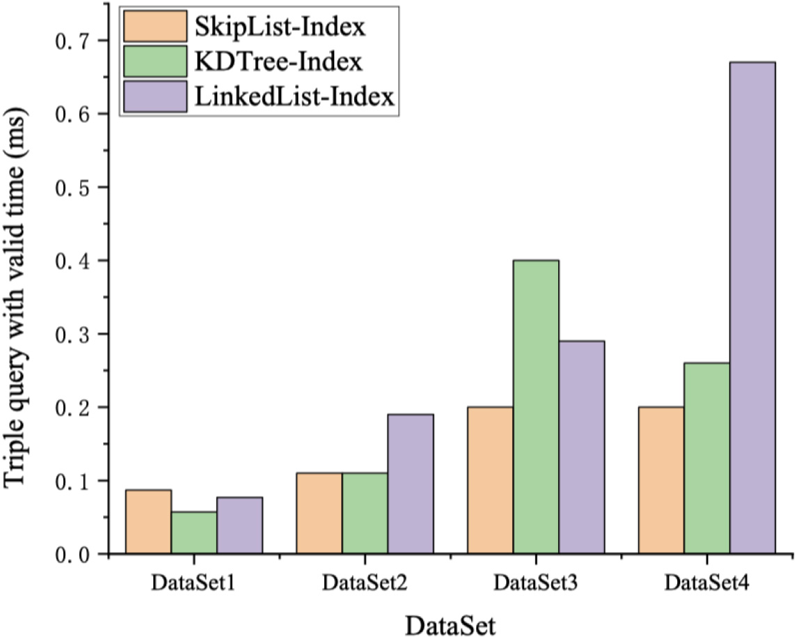

Figure 5 shows the query performance of the single triple pattern on the four data sets of Table 2, where the valid time is known, and the indexes are our SkipList-index, the kdTree-index [20], and the LinkedList-index, respectively. The results are the average time taken by the execution of five queries.

In Fig. 5, the query time of the linked list index increases with the increase of the size of the data set, and the performance of our skip list query is relatively stable. Because the K-D tree index is a two-level index and the time is the first-level index, the query speed is advantageous when the time element is known. However, when the size of data sets is large, the query time of our skip list is still less than the K-D tree index.

Figure 6.

Triple query result when the valid time is unknown.

Figure 6 shows the query of a single triplet when the valid time is unknown. When the time is unknown, the performance of the K-D tree index drops significantly. This is because it uses time as the first-level index. When the time is unknown, the query needs to be traversed in the tree, so the time consumption will increase. For our skip list index, the performance can be guaranteed by selecting the correct list. Although the linked list index can also select the list according to different situations, the query time is also longer than the skip list index due to the limitation of the linked list structure.

Figure 7.

The result of bitemporal triple query (i.e., valid and transaction time are known).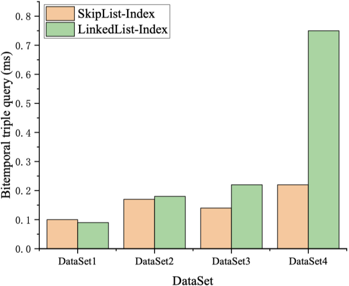

To further prove the effectiveness of the index in the bitemporal state, we show the experimental results when the valid time and transaction time are known in Fig. 7. Because the K-D tree index is a single temporal index and cannot support a bitemporal index, Fig. 7 only shows the results of the skip lists index and the linked list index.

5.1.2 Multiple triple query performance

Being similar to the single triple query above, the multiple triple query mode is also divided into two situations: when the time is known and when the time is unknown. LUBM has a commended list of fourteen queries that consider different aspects related to query optimizations. To test the effect of multiple triple query (i.e., the path query and the star query as mentioned in Section 5.1), we selected several queries from fourteen queries for testing.

Figure 8.

A multiple triple path query Query1.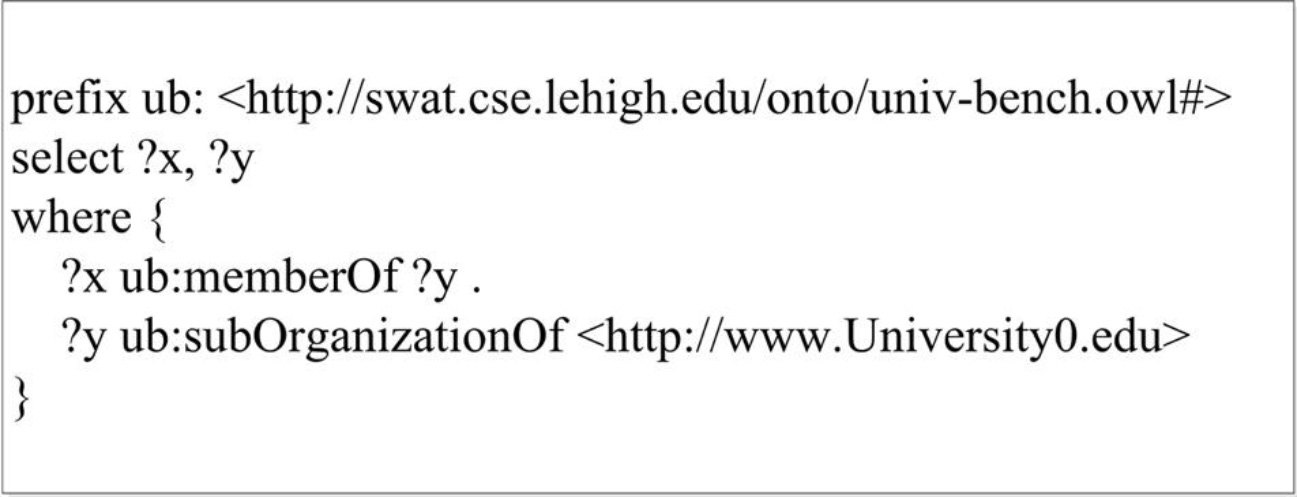

Figure 9.

The result of Query1.

Figure 8 gives a path query (called Query1 for short), which consists of several connected triple patterns that form a path. The query result is shown in Fig. 9.

As can be seen from Fig. 9, when the temporal information is unknown, the K-D tree index can only query data by traversing the index, so the query efficiency will decrease significantly. Our bitemporal index SkipList-Index based on skip lists can match the appropriate index through the basic query mode, thereby achieving the purpose of fast query.

Figure 10.

A multiple triple star query Query2.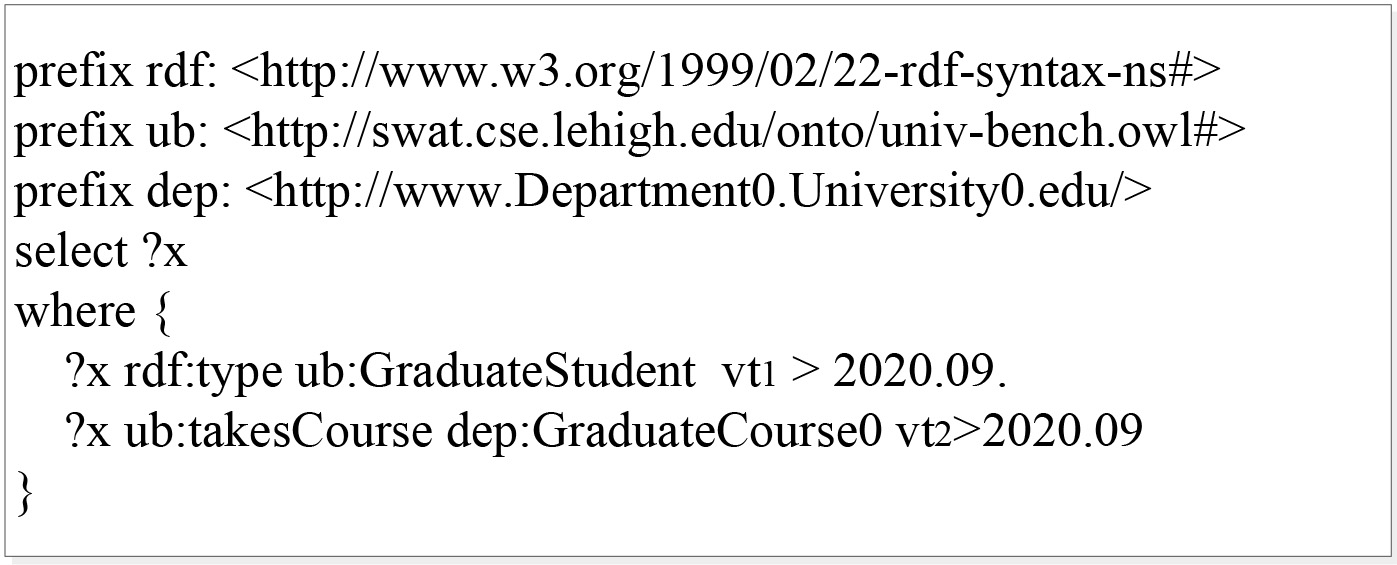

Moreover, Fig. 10 shows the benchmark query used in our star query evaluation (called Query2 for short), where the valid time is known.

Figure 11.

The result of Query2.

For Query2, we do not perform two queries separately and take the intersection of the results. Because two triples have their respectively specified time, and the number of triples at a specified time is much smaller than the number of triples in the entire data set. Therefore, after processing the first triple, only the result of the first triple query is brought into the second triple for judgment. The result of Query2 is shown in Fig. 11.

Figure 12.

A more complex multiple triple star query Query3.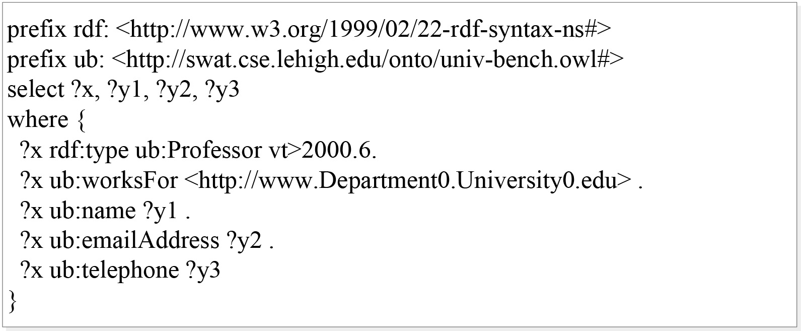

Figure 13.

The result of Query3.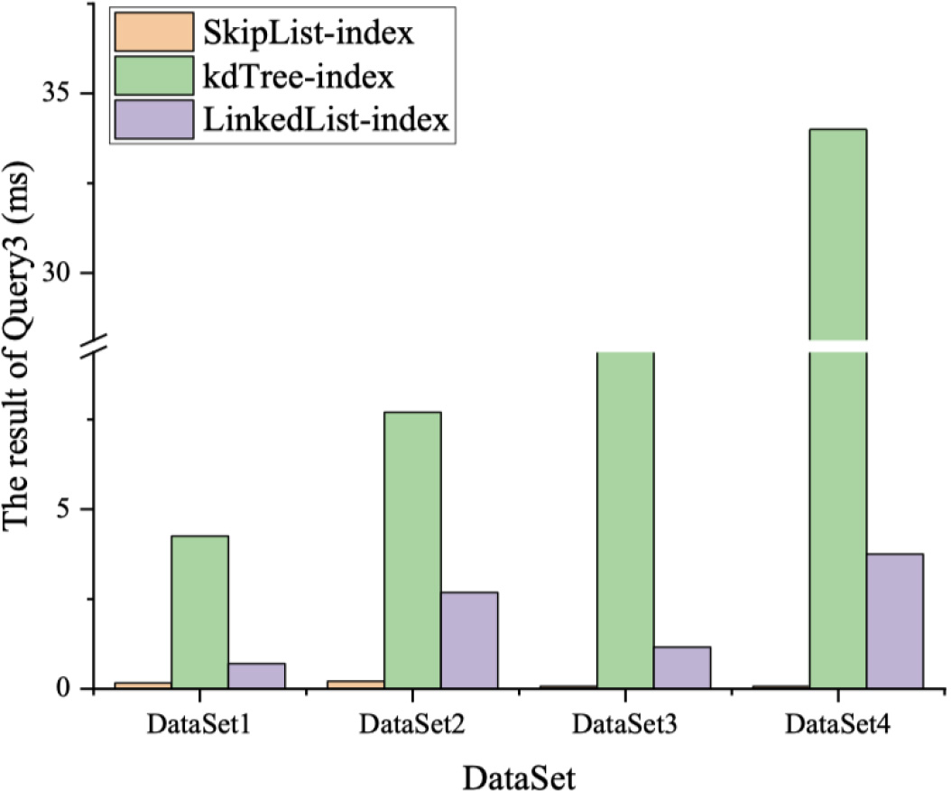

A more complex star query is selected for evaluation to further prove the effectiveness of the index, we call it Query3. Query3 is shown in Fig. 12 and the result of Query3 is shown in Fig. 13. In addition to the complexity of the query, another difference between Query3 and Query2 is that Query3 only specifies the time of one triple instead of specifying the time of all triples.

It can be seen in Fig. 13 that the advantage of the skip list index is evident when the query becomes complicated and not the times of all triples are known. This is because the skip list index is indexed for various situations, rather than only considering the time-known situation. The performance of the K-D tree index degrades a lot because the tree needs to be traversed when the time is unknown and the time spent on the traversal is huge.

5.2 Index building and storage performance

Figure 14.

The building time of different indexes on four data sets.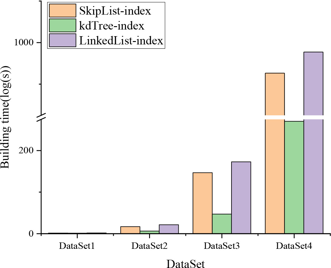

In this subsection, we further evaluate the index performance from the building time and the storage space. First, we evaluate the time of building indexes over different data sets. Because the number of triples in the data set varies greatly, the building time of different data sets are also very different. To make the comparison more clearly, a logarithmic scale is used in Fig. 14. Note that the skip list index and the linked list index consider more situations, and indexes for the different situations need to be established respectively, but the K-D tree index is to build a global index, so the building time of the skip list index and the linked list index is slightly longer than the K-D tree index.

Figure 15.

The storage space of index.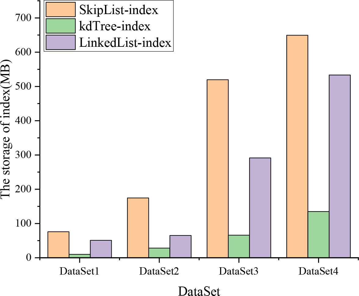

Next, we evaluate the storage space of indexes over different data sets. As shown in Fig. 15, since the skip list index not only needs to store basic triple information but also needs to additionally store the next-hop information of each node, more storage space is required for the skip list index than the linked list index and the K-D tree index.

Based on all of the experiments on different data sets in this section, we can find that our bitemporal index can support more kinds of RDF queries. Moreover, although in terms of building time and storage space, our skip list index is not dominant compared to other indexes, the query regarding to different queries (including the single triple pattern and the multiple triple pattern) are more effective.

6. Conclusions and future work

In this paper we propose an efficient index for bitemporal RDF query. We innovatively introduce and re-design skip list structure into the bitemporal RDF query, and cover almost all query patterns with as few indexes as possible. In particular, although the proposed index is used to index temporal RDF, the index also takes into account the performance of standard RDF queries when the time element is unknown. Finally, we run experiments with synthetic data sets of different sizes using the Lehigh University Benchmark (LUBM), and the results show that the proposed index is scalable and effective. Compared with other indexes that do not consider the time or only consider the time element is known, the index proposed in our work is more comprehensive and effective.

In future work, we will further discuss and investigate the following issues in depth. First of all, our method proposed in this paper builds different indexes for different situations in order to cover more basic query modes. However, at the same time, the index also needs to store data and pointers in different modes, so the space occupied is also slightly more. In our near future work, we will consider introducing technologies such as caching and space compression to solve the issue of index storage space. In addition, our bitemporal RDF experimental data set is constructed on the basis of the widely used RDF benchmark LUBM, and in future work we will consider and conduct more comprehensive and in-depth experiments on real scene data.

Footnotes

Acknowledgments

The authors sincerely thank the anonymous referees for their valuable comments and suggestions, which improved the paper. The work is supported by the National Natural Science Foundation of China (62276057) and the Fundamental Research Funds for the Central Universities (No. N2216008).

References

Brisaboa

N.R.

Cerdeira-Pena

Bernardo

G.D.

and Faria

, Revisiting compact RDF stores based on K2-trees, in: 2020 Data Compression Conference (DCC), Snowbird, UT, USA, (2020), 123–132.

RDF 1.1 Primer, W3C Working Group. [Online]. Available: http://www.w3.org/TR/2014/NOTE-rdf11-primer-20140225/, date of access: 2022-06-20.

Gutierrez

Hurtado

and Vaisman

, Introducing time into RDF, IEEE Transactions on Knowledge and Data Engineering 19(2) (2007), 207–218.

Analyti

and Pachoulakis

, A survey on models and query languages for temporally annotated RDF, International Journal of Advanced Computer Science and Applications 3(9) (2012), 28–35.

Gutierrez

Hurtado

and Vaisman

, Temporal RDF, in: The Semantic Web: Research and Applications, ESWC 2005 Gómez-Pérez

Euzenat

, ed., Springer, Berlin, Heidelberg, (2005), 93–107.

Zhang

Z.Y.

Peng

D.H.

and Cheng

J.W.

, RDF for temporal data management – a survey, Earth Science Informatics 14 (2021), 563–599.

Böhlen

M.H.

Dignös

Gamper

and Jensen

C.S.

, Temporal data management – an overview, in: Business Intelligence and Big Data, eBISS 2017 Zimányi

, ed., Springer, Cham, (2018), 51–83.

Bellamy-McIntyre

, LSPARQL: Transaction Time Queries in RDF, The University of Auckland, (2020).

Meijer

, Bi-VAKs: Bi-temporal Versioning Approach for Knowledge Graphs, Delft University of Technology, (2022).

10.

Han

and Yan

, Modeling and querying temporal RDF knowledge graphs with relational databases, Journal of Intelligent Information Systems 61(1) (2023), 1–41.

11.

, BiTRDF: Extending Rdf for Bitemporal Data, City University of New York, (2022).

12.

Udrea

Pugliese

and Subrahmani

V.S.

, GRIN: a graph based RDF index, in: AAAI Conference on Artificial Intelligence (AAAI), (2007), 1465–1470.

13.

Pugh

, Skip lists: a probabilistic alternative to balanced trees, Communications of the ACM 33(6) (1990), 668–676.

14.

Ali

Saleem

Yao

Hogan

and Ngomo

, A survey of RDF stores & sparql engines for querying knowledge graphs, VLDB 31 (2022), 1–26.

15.

Neumann

and Weikum

, RDF-3X: a risc-style engine for RDF, Proceedings of the VLDB Endowment 1(1) (2008), 647–659.

16.

Madduri

and Wu

, Massive-scale RDF processing using compressed bitmap indexes, in: International Conference on Scientific and Statistical Database Management, Springer, Berlin, Heidelberg, (2011), 470–479.

17.

Brisaboa

N.R.

et al., A compact RDF store using suffix arrays, in: International Symposium on String Processing and Information Retrieval, Springer, Cham, (2015), 103–115.

18.

Pugliese

Udrea

and Subrahmanian

V.S.

, Scaling RDF with time, in: Proceedings of the 17th international conference on World Wide Web (2008), 605–614.

19.

Yan

Zhao

and Ma

, Indexing temporal RDF graph, Computing 101(10) (2019), 1457–1488.

20.

Zhao

and Yan

, A methodology for indexing temporal RDF data, Journal of Information Science and Engineering 35(4) (2019), 923–934.

21.

Tappolet

and Bernstein

, Applied temporal RDF: efficient temporal querying of RDF data with SPARQL, in: ESWC 2009: The Semantic Web: Research and Applications (2009), 308–322.

22.

Guo

Pan

and Heflin

, LUBM: a benchmark for OWL knowledge base systems, Journal of Web Semantics 3(2–3) (2005), 158–182.

23.

Bae

et al., Indexing and querying algorithm based on structure indexing for managing massive-scale RDF data, Journal of Intelligent & Fuzzy Systems 27(2) (2014), 575–587.