A modified belief rule based model for uncertain nonlinear systems identification

Abstract

The belief rule based (BRB) methodology is developed from the traditional IF–THEN rule based system and evidential reasoning (ER) approach. It can be used to model complicated nonlinear causal relationships between antecedent attributes and consequents under different types of uncertainty. In this paper, we present a new BRB structure for modelling uncertain nonlinear systems. It uses the weighted averaging operator to replace the ER approach in the inference process. With this change, the BRB structure could be simplified and faster speeds are obtained in both training and inference process, while universal approximation capability is maintained. By using the consequents of the new BRB model, an approach for reducing possibly redundant referential values of antecedent attributes is proposed for point estimate. Case studies are conducted on three well known benchmark datasets to compare the new model with the existing BRB model and other methods in the literature. Experimental results demonstrate the capability of the proposed method for identification of nonlinear systems.

Keywords

Belief rule base system identification evidence theory weighted average attribute reduction

1 Introduction

Identification of a nonlinear system is of funda-mental importance in predictive control, fault diagnosis and signal processing, etc., since most real-life systems are nonlinear. They are often associated with uncertainties due to noises, unpredictable disturbance, uncertain physical parameters and incomplete knowledge. Those uncertainties cause a great difficulty in applying traditional identification techniques. Over the past few decades, extensive studies have been conducted for identifying uncertain nonlinear systems, especially with the advent of neural network [12 , 18] and fuzzy rule based system techniques [21 , 28]. However, these methods usually involve some restrictive assumptions, such as Gaussian distributed noises, deterministic disturbances and bounded uncertain parameters [2]. Besides, fuzzy models for lower and upper bounds are independent from each other in some interval estimate methods, and it may incur improper identification results with invalid bounds if no enough training data is available in some regions of the input space [25].

Recently, the BRB methodology is developed on the basis of D-S evidence theory [22], decision theory [19], traditional IF-THEN rule based systems [13, 16] and relevant artificial intelligence techniques [9, 15]. In a BRB system, various types of information and knowledge with uncertainties can be represented using belief structures, and a belief rule is designed with belief degrees embedded in its possible consequents. The belief structure used in both belief rules and inference processes provides a unified scheme to model uncertain system outputs caused by vagueness, fuzziness, or incompleteness, etc [4]. Because of its advantages of dealing with uncertainty, it has been successfully applied in various areas, such as fault diagnosis [30], multi-attribute decision analysis [11] and classification [1]. It also provides an alternative for the identification of nonlinear systems [4 , 23].

Making use of BRB’s capability of approximation and dealing with uncertainty, Chen et al. [4] proposed three approaches to construct BRB models for uncertain nonlinear systems. Like all other BRB models, ER approach [32] is applied to aggregate all activated belief rules to generate the final inference output. In a BRB model, most parameters come from the belief distributions of rule consequents. If this part of parameters can be cut down, much convenience can be brought to the training and inference process.

A BRB model can approximate any real continuous function over a compact subset and its accuracy could be improved by using more referential values for antecedent attributes [5]. However, the increase of referential values would cause problems such as the increase of belief rules and overfitting of the training data. Thus a tradeoff should be made and redundant referential values should be abandoned to achieve a good performance. Zhou et al. [33] defined the statistical utility to prune insignificant rules. Chang et al. [3] conducted a comparative study of four techniques for reducing redundant belief rules when the rules are given by expert. These methods depend on extra information or knowledge from experts. Wang et al. [29] put forward an objective rule reduction method based on rough set theory. However, these aforementioned methods are not designed for the identification problem in which belief rules are constructed directly using combinations of antecedent attributes and are generally not contradict.

The main contribution of this work is two folds. First, we investigate the feasibility of using an alternative combination rule to aggregate the activated belief rules. The weighted averaging operator is chosen after analysis and it is shown that this combination rule can simplify the structure of BRB model significantly while maintaining the universal approximation capability. Second, an approach for attribute reduction is proposed by use of the new BRB structure. Three commonly used case studies are exploited to demonstrate the performance of the proposed method.

The rest of this paper is organized as follows. Section 2 briefly reviews the BRB model. Section 3 states the motivation of this paper. Section 4 details a new BRB model along with an attribute reduction approach. Section 5 presents several numerical studies to demonstrate the approximation capability of the new BRB model and the attribute reduction approach. Finally a conclusion is drawn in section 6.

2 Belief rule based systems

To simulate an uncertain nonlinear system, a BRB model consists of two parts, first establishing the belief rule base, and then aggregating all activated belief rules using the ER approach.

2.1 Belief rule base

A belief rule base consists of a finite number of belief rules. Formally, a belief rule is defined as follows [31]: $R_{k} : \begin{matrix} IF x_{1} is A_{1}^{k} \land x_{2} is A_{2}^{k} \land \dots \land x_{M_{k}} is A_{M_{k}}^{k}, \\ THEN {(D_{1}, β_{1, k}), \dots, (D_{N}, β_{N, k})}, \sum_{n = 1}^{N} β_{n, k} \leq 1, \\ with rule weight θ_{k}, and attribute \\ weight δ_{1, k}, \dots, δ_{M_{k}, k}, k \in {1, \dots, L} . \end{matrix}$ (1) where x₁, x₂, . . . , x_{M
_k} denote the antecedent attributes in the kth rule, and they are a subset of all the antecedent attributes X = {x_i ; i = 1, . . . , M}. $A_{i}^{k} (i = 1, . . ., M_{k})$ is the referential value taken by the ith antecedent attribute in the kth rule and $A_{i}^{k} \in A_{i}$ . A_i = {A_i,j ; j = 1, . . . , J_i} denotes the set of referential values for the ith antecedent attribute and J_i is the number of the referential values. β_n,k (n = 1, . . . , N ; k = 1, . . . , L) represents the belief degree to which the element D_n is believed to be the consequent. The kth rule is said to be complete if $\sum_{n = 1}^{N} β_{n, k} = 1$ ; otherwise, it is incomplete. θ_k is the relative weight of the kth rule, and δ_{M_k,k} represents the relative weight of attribute in the kth rule.

2.2 Inference process

To estimate the output given an input vector x (t) = {x_i (t) ; i = 1, . . . , M} at sampling time t, each input x_i (t) needs to be transformed to the following belief distribution using referential values of the ith antecedent. For simplicity, x_i is used to represent x_i (t) henceforth. $S (x_{i}) = {(A_{i, j}, α_{i, j}), j = 1, \dots, J_{i}}$ (2) where $\begin{matrix} α_{i, j} = \frac{A_{i, j + 1} - x_{i}}{A_{i, j + 1} - A_{i, j}} and \\ α_{i, j + 1} = 1 - α_{i, j}, if A_{i, j} ⩽ x_{i} ⩽ A_{i, j + 1} \\ α_{i, j^{'}} = 0, j^{'} \in {1, \dots, J_{i}}, j^{'} \neq j, j + 1 \end{matrix}$

Here, α_i,j represents the similarity degree to which the input value x_i matches the referential value A_i,j. After all the inputs are transformed into belief distributions, the activation weight of the kth belief rule can be calculated as follows: $w_{k} (x) = \frac{θ_{k} \prod_{i = 1}^{M_{k}} (α_{i, j}^{k})^{\bar{δ_{i}}}}{\sum_{l = 1}^{L} [θ_{l} \prod_{i = 1}^{M_{k}} (α_{i, j}^{l})^{\bar{δ_{i}}}]}$ (3) $where \bar{δ_{i}} = \frac{δ_{i}}{{max}_{i = 1, \dots, M_{k}} {δ_{i}}}$ (4)

Note that in Equation (3) the attribute weights are assumed to be identical in all belief rules. Further, the belief degrees on the inference output can be generated through the aggregation of all activated belief rules using the ER approach [32]. $\begin{matrix} β_{n} (x) & = μ^{- 1} \times [\prod_{k = 1}^{L} (w_{k} (x) β_{n, k} + 1 - w_{k} (x) \sum_{i = 1}^{N} β_{i, k}) \\ - \prod_{k = 1}^{L} (1 - w_{k} (x) \sum_{i = 1}^{N} β_{i, k})] \end{matrix}$ (5) $\begin{matrix} β_{D} (x) & = μ^{- 1} \times [\prod_{k = 1}^{L} (1 - w_{k} (x) \sum_{i = 1}^{N} β_{i, k}) \\ - \prod_{k = 1}^{L} (1 - w_{k} (x))] \end{matrix}$ (6) where $\begin{matrix} μ & = \sum_{j = 1}^{N} \prod_{k = 1}^{L} (w_{k} (x) β_{j, k} + 1 - w_{k} (x) \sum_{i = 1}^{N} β_{i, k}) \\ - (N - 1) \prod_{k = 1}^{L} (1 - w_{k} (x) \sum_{i = 1}^{N} β_{i, k}) - \prod_{k = 1}^{L} (1 - w_{k} (x)) \end{matrix}$ and β_D ( x ) represents the remaining belief degree unassigned to any known D_n and $\sum_{n = 1}^{N} β_{n} (x) + β_{D} (x) = 1$ . As a result, the inference output can be represented as the following belief distribution. $S (\hat{y} (x)) = {(D_{n}, β_{n} (x)); n = 1, \dots, N}$ (7)

Suppose that the utility of each consequent element D_n is denoted by u (D_n) and all belief rules are complete. The inference output can be calculated by $\hat{y} (x) = \sum_{n = 1}^{N} u (D_{n}) β_{n} (x)$ (8)

In uncertain nonlinear systems, belief rules may not all be complete, and then we may have β_D ( x ) >0. In this case, β_D ( x ) can be used to quantify the extent of uncertainty associated with each consequent element, and a BRB utility interval could be established to represent the uncertain output, characterized by the maximum, minimum and average utilities of $\hat{y} (x)$ defined as follows. ${\hat{y}}_{\max} (x) = \sum_{n = 1}^{N} u (D_{n}) β_{n} (x) + u (D_{n}) β_{D} (x)$ (9) ${\hat{y}}_{\min} (x) = \sum_{n = 1}^{N} u (D_{n}) β_{n} (x) + u (D_{1}) β_{D} (x)$ (10) ${\hat{y}}_{ave} (x) = \frac{{\hat{y}}_{\min} (x) + {\hat{y}}_{\max} (x)}{2}$ (11)

2.3 Training of BRB systems

When observed input–output data pairs are available, optimal learning methods can be designed to train the BRB parameters. In [4], three different training approaches are introduced with the following objective functions, respectively. $min_{P} ξ_{1} (P) = \frac{1}{T} \sum_{t = 1}^{T} ({\hat{y}}_{ave} (x_{t}) - y_{t})^{2}$ (12)

$min_{P} max_{x_{t}} ξ_{2} (P) = (| y_{t} - {\hat{y}}_{\min} (x_{t}) |, | {\hat{y}}_{\max} (x_{t}) - y_{t} |)$ (13)

$min_{P} ξ_{3} (P) = \frac{1}{L} \sum_{k = 1}^{L} (1 - \sum_{n = 1}^{N} β_{n, k})$ (14) where P = 〈A_i,j, θ_k, δ_i, β_n,k, u (D_n) 〉. In the training process, the parameters in terms of physical meanings must satisfy the following constraints [6, 31]: $0 \leq β_{n, k} \leq 1, n = 1, \dots, N; k = 1, \dots, L$ (15-a) $\sum_{n = 1}^{N} β_{n, k} \leq 1, k = 1, \dots, L$ (15-b) $0 \leq θ_{k} \leq 1, k = 1, \dots, L$ (15-c) $0 \leq δ_{i} \leq 1, i = 1, \dots, M$ (15-d) $A_{i, j} < A_{i, j + 1}, i = 1, \dots, M; j = 1, \dots, J_{i} - 1$ (15-e) $u (D_{i}) < u (D_{j}) if i < j, i, j = 1, \dots, N$ (15-f)

3 Motivation

More referential values for antecedent attributes usually can improve the approximation accuracy. Meanwhile, too many referential values would increase the complexity of the constructed model and lead to overfitting if there are noises in data. This problem is illustrated by the following example.

Example 1. Consider the following nonlinear function $y = \frac{sinx}{x} + ε$ (16)

where ε is Gaussian noise with zero mean and variance δ = 0.05 [4]. To construct a BRB model to simulate this system with noises, 4 referential values of the input variable x within the interval [0, 10] are initially defined as {0, 3, 7, 10}. A training dataset with 100 data points is generated from the nonlinear function. Table 1 lists the trained belief rule base.

Table 1

Trained belief rule base in Example 1

R _k	θ _k	x (A_j)	{D_i} = {-0.5, - 0.1933, 0.0807, 0.9687, 1.0687}, δ = 0.8788
1	0.8584	0	{(D₁, 0) , (D₂, 0) , (D₃, 0) , (D₄, 0.7645) , (D₅, 0.2355)}
2	0.8812	4.3038	{(D₁, 0.5888) , (D₂, 0.2784) , (D₃, 0) , (D₄, 0.1328) , (D₅, 0)}
3	0.7451	7.3875	{(D₁, 0) , (D₂, 0.6168) , (D₃, 0.1692) , (D₄, 0) , (D₅, 0.2141)}
4	0.8419	10	{(D₁, 0.6971) , (D₂, 0) , (D₃, 0) , (D₄, 0) , (D₅, 0.3029)}

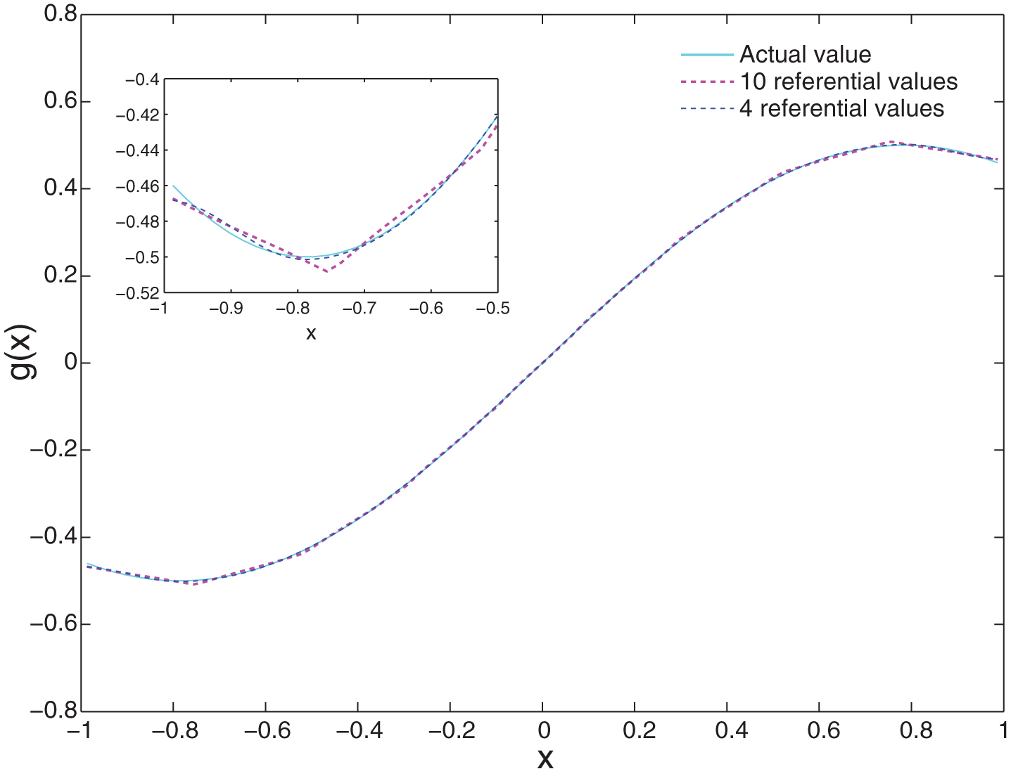
If we use 6 referential values for x with initial values {0, 2, 4, 6, 8, 10}, another BRB model could be established with the same training dataset. Figure 1 illustrates the estimated outputs of the trained BRB models with 4 and 6 referential values. The mean square error (MSE) between the actual output and the estimated outputs are 0.00212 and 0.00195, respectively. The BRB model with 6 referential values has a slightly better performance in terms of MSE. Nevertheless, different belief rules would be activated when x increase from smaller than to bigger than a referential value, which may make the curve not smooth at each referential value. We can see from the figure that the blue curve is very smooth while the pink curve has several turn points. As a result, appropriate number of referential values should be used and an approach for reducing redundant referential values is necessary.

Fig.1

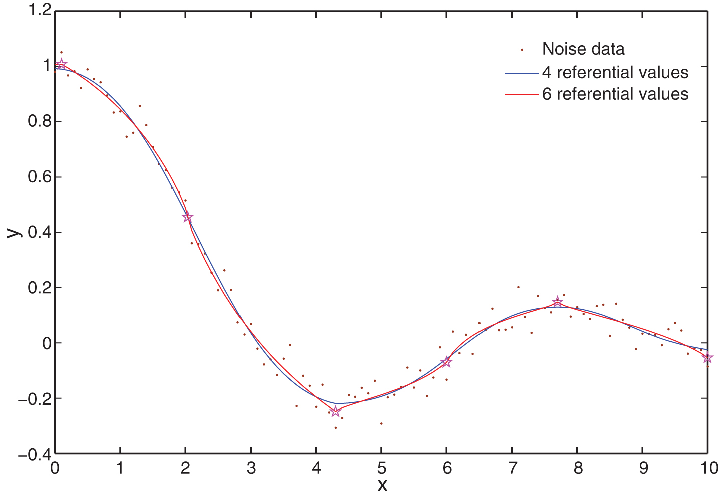
Estimated output with different numbers of referential values.

Suppose m₁ and m₂ are two basic belief assignments (BBAs). The degree of conflict between them is classically defined as [22] $K = \sum_{A, B \subset Θ, A \cap B = \emptyset} m_{1} (A) m_{2} (B)$ (17)

By this definition, we can calculate the degrees of conflict between each pair of adjacent belief rules in Table 1: K₁₂ = 0.8985, K₂₃ = 0.8283, K₃₄ = 0.9352. It implies that the belief distribution of activated rules are always in high conflict. In fact, this is not a unique case. Consider the trained belief rule bases in Table 3, Table 5(a) and Table 5(b) of literature [4], the average degrees of conflict of adjacent belief rules are 0.5920, 0.6391 and 0.6953, respectively. Note that belief rules are incomplete in these models, otherwise the degrees of conflict may be even higher. ER approach can achieve a good performance when aggregating conflicting BBAs with various weights, and it is applied in the inference process of BRB models. A variety of alternative rules are also capable of aggregating conflicting belief functions. Murphy discussed this problem and proposed an averaging method [17], and Deng et al. put forward a modified approach [8]. In this paper, we therefore investigate the feasibility of using weighted averaging operator in the inference process.

Table 2

Initial belief rule base for Box-Jenkins gas furnace example

R _k	θ _k	u (t - 4) ∧ y (t - 1)	{D₁, D₂, D₃, D₄, D₅}	v _k
1	1	NL ∧ VL	{(D₁, 0.1) , (D₂, 0.9) , (D₃, 0) , (D₄, 0) , (D₅, 0)}	48.6
2	1	NL ∧ L	{(D₁, 0) , (D₂, 0.5) , (D₃, 0.5) , (D₄, 0) , (D₅, 0)}	51.0
3	1	NL ∧ M	{(D₁, 0) , (D₂, 0) , (D₃, 0.5) , (D₄, 0.5) , (D₅, 0)}	55.0
4	1	NL ∧ H	{(D₁, 0) , (D₂, 0) , (D₃, 0) , (D₄, 0.3) , (D₅, 0.7)}	59.8
5	1	NL ∧ VH	{(D₁, 0) , (D₂, 0) , (D₃, 0) , (D₄, 0) , (D₅, 1)}	61.0
6	1	NS ∧ VL	{(D₁, 0.25) , (D₂, 0.75) , (D₃, 0) , (D₄, 0) , (D₅, 0)}	48.0
7	1	NS ∧ L	{(D₁, 0) , (D₂, 0.75) , (D₃, 0.25) , (D₄, 0) , (D₅, 0)}	50.0
8	1	NS ∧ M	{(D₁, 0) , (D₂, 0) , (D₃, 0.5) , (D₄, 0.5) , (D₅, 0)}	55.0
9	1	NS ∧ H	{(D₁, 0) , (D₂, 0) , (D₃, 0) , (D₄, 0.7) , (D₅, 0.3)}	58.2
10	1	NS ∧ VH	{(D₁, 0) , (D₂, 0) , (D₃, 0) , (D₄, 0.25) , (D₅, 0.75)}	60.0
11	1	Z ∧ VL	{(D₁, 0.5) , (D₂, 0.5) , (D₃, 0) , (D₄, 0) , (D₅, 0)}	47.0
12	1	Z ∧ L	{(D₁, 0) , (D₂, 0.9) , (D₃, 0.1) , (D₄, 0) , (D₅, 0)}	49.4
13	1	Z ∧ M	{(D₁, 0) , (D₂, 0) , (D₃, 0.95) , (D₄, 0.05) , (D₅, 0)}	53.2
14	1	Z ∧ H	{(D₁, 0) , (D₂, 0) , (D₃, 0) , (D₄, 1) , (D₅, 0)}	57.0
15	1	Z ∧ VH	{(D₁, 0) , (D₂, 0) , (D₃, 0) , (D₄, 0.5) , (D₅, 0.5)}	59.0
16	1	PS ∧ VL	{(D₁, 0.75) , (D₂, 0.25) , (D₃, 0) , (D₄, 0) , (D₅, 0)}	46.0
17	1	PS ∧ L	{(D₁, 0.3) , (D₂, 0.7) , (D₃, 0) , (D₄, 0) , (D₅, 0)}	47.8
18	1	PS ∧ M	{(D₁, 0) , (D₂, 0.35) , (D₃, 0.65) , (D₄, 0) , (D₅, 0)}	51.6
19	1	PS ∧ H	{(D₁, 0) , (D₂, 0) , (D₃, 0.5) , (D₄, 0.5) , (D₅, 0)}	55.0
20	1	PS ∧ VH	{(D₁, 0) , (D₂, 0) , (D₃, 0) , (D₄, 0.75) , (D₅, 0.25)}	58.0
21	1	PL ∧ VL	{(D₁, 1) , (D₂, 0) , (D₃, 0) , (D₄, 0) , (D₅, 0)}	45.0
22	1	PL ∧ L	{(D₁, 0.75) , (D₂, 0.25) , (D₃, 0) , (D₄, 0) , (D₅, 0)}	46.0
23	1	PL ∧ M	{(D₁, 0) , (D₂, 0.75) , (D₃, 0.25) , (D₄, 0) , (D₅, 0)}	50.0
24	1	PL ∧ H	{(D₁, 0) , (D₂, 0) , (D₃, 0.75) , (D₄, 0.25) , (D₅, 0)}	54.0
25	1	PL ∧ VH	{(D₁, 0) , (D₂, 0) , (D₃, 0) , (D₄, 1) , (D₅, 0)}	57.0

Table 3

Comparison results for the Box-Jenkins gas furnace example

Model	No. of	MSE	MSE	Training
	Ref.	(Training)	(Testing)	time(s)
BRB	3 × 3	0.0700	0.4137	59.6
	4 × 4	0.0652	0.3543	138.1
	5 × 5	0.0556	0.3149	297.3
modified	3 × 3	0.0796	0.4739	3.3
BRB	4 × 4	0.0600	0.3618	6.1
	5 × 5	0.0621	0.2868	9.7

Table 4

Comparison results for two dimensional Sinc function example

Model	No. of rules	MSE
Evsukoff [10]	49	0.001
Rezaee [20]	14	0.0001
Uncu and Türksen [27]
DIT2-LFR	-	0.0024
DIT2-MFR	-	0.0011
DIT2-TSFR	-	0.0034
	6 × 6	4.8 × 10^-4
modified BRB model	7 × 7	9.2 × 10^-6
	9 × 9	9.6 × 10^-5

Table 5

Initial modified belief rule base for point estimate

R _k	1	2	3	4	5	6	7	8	9	10
θ _k	1	1	1	1	1	1	1	1	1	1
x (A_j)	–1	–0.8	–0.6	–0.3	–0.1	0.1	0.3	0.6	0.8	1
v _k	–0.6	–0.5	–0.4	–0.3	–0.1	0.1	0.3	0.4	0.5	0.6

Table 6

Initial modified belief rule base for interval estimate

R _k	1	2	3	4	5	6	7	8
θ _k	1	1	1	1	1	1	1	1
x (A_j)	–1	–0.7	–0.4	–0.1	0.2	0.4	0.7	1
v _k	–0.5	–0.4	–0.3	–0.1	0.1	0.3	0.4	0.5
β _k	0.1	0.2	0.1	0.2	0.1	0.1	0.2	0.1

4 A modified belief rule based model

In this section, the BRB model using weighted averaging operator in its inference process is presented. Based on this simplified model, an approach is put forward to reduce the possibly redundant referential values of antecedent attributes.

4.1 Inference using weighted averaging operator

Aggregating the activated belief rules with weighted averaging operator instead of ER approach would weaken the nonlinearity of the BRB model, especially in the case of one input. In order to improve its capability of approximating nonlinear systems, we use a nonlinear formula rather than Equation (2) when transforming the input x into belief distribution. $\begin{matrix} α_{i, j} = 0.5 \cos \frac{(A_{i, j} - x_{i}) π}{A_{i, j + 1} - A_{i, j}} + 0.5 and \\ α_{i, j + 1} = 1 - α_{i, j}, if A_{i, j} \leq x_{i} \leq A_{i, j + 1} \\ α_{i, j^{'}} = 0, j^{'} \in {1, \dots, J_{i}}, j^{'} \neq j, j + 1 \end{matrix}$

The belief degrees on the inference output generated by weighted averaging operator is as follows: $β_{n} (x) = \sum_{k = 1}^{L} w_{k} (x) β_{n, k}, n = 1, \dots, N$ (18)

Let Γ = [ β₁ , ⋯ , β_L ]^T, β_k = [β_1,k, ⋯ , β_N,k]^T, w ( x ) = [w₁ ( x ), ⋯, w_L ( x )]^T and u = [u (D₁) , ⋯ , u (D_N)]^T. The inference output given by Equation (8) can be transformed into $\hat{y} (x) = \sum_{n = 1}^{N} β_{n} (x) u (D_{n}) = w^{T} (x) Γ u$ (19)

Let v = Γu . Then v is a L × 1 constant vector independent of the input x once the design parameters of a BRB model are determined, and v_i ∈ [u (D₁) , u (D_n)]. Clearly, to train parameters in Γ and u is equivalent to train the variable v . As a result, the belief rules (1) could be simplified as follows:

$R_{k} : \begin{matrix} IF x_{1} is A_{1}^{k} \land x_{2} is A_{2}^{k} \land \dots \land x_{M_{k}} is A_{M_{k}}^{k}, \\ THEN (v_{k}, β_{k}), β_{k} \leq 1, \\ with rule weight θ_{k}, and attribute weight \\ δ_{1, k}, δ_{2, k}, \dots, δ_{M_{k}, k}, k \in {1, 2, \dots, L} . \end{matrix}$ (20)

The inference output could then be calculated as ${\hat{y}}_{\max} (x) = w^{T} (x) v + u (D_{N}) β_{D}$ (21) ${\hat{y}}_{\min} (x) = w^{T} (x) v + u (D_{1}) β_{D}$ (22) ${\hat{y}}_{ave} (x) = \frac{{\hat{y}}_{\max} (x) + {\hat{y}}_{\min} (x)}{2}$ (23) where β_D= w ^T( x ) ( 1 _L - β ), 1 _L is a column vector of L dimension, and β =[β₁, ⋯, β_L]^T.

If all rules are complete, i.e., β_k = 1, k ∈ {1, ⋯ , L}, then the inference output could be unified as follows $\hat{y} (x) = w^{T} (x) v$ (24)

In the BRB model (1), there are $\sum_{i = 1}^{M} J_{i} + N + M + (N + 1) L$ design parameters in total. In the modified model (20), the number of design parameters is $\sum_{i = 1}^{M} J_{i} + M + 3 L$ . Thus more than (N - 2) L parameters are reduced in the general case and (N - 1) L parameters can be reduced when all rules are complete. As M and N are very small compared with the number of rules which is designed to be $L = \prod_{i = 1}^{M} J_{i}$ , usually more than half of the parameters can be reduced. The reduction of design parameters and the usage of weighted averaging operator in the modified BRB model not only reduce the model complexity, but also significantly cut down the time needed for training and inference process. Besides, it is easier to set initial values for these design parameters.

In the training of BRB models, parameters must satisfy the constraints (15-a)–(15-f). When training the modified BRB system, constraints (15-a),(15-b) and (15-f) should be replaced by the following inequalities. $0 \leq β_{k} \leq 1, k = 1, \dots, L$ (25) $β_{k} u (D_{1}) \leq v_{k} \leq β_{k} u (D_{N}), k = 1, \dots, L$ (26)

Though a different inference rule is used, the modified BRB model possesses the universal approximation capability. According to the proof provided in [5], the Stone-Weierstrass theorem [7] is applied to prove its approximation capability.

Theorem 1. For any given real continuous function g ( x ) on a compact domain U ⊆ R^m and ∀ε > 0, there exists a modified BRB model f ( x ) ∈ F ( x ) such that $| | g (x) - f (x) | |_{\infty} < ε$ where F ( x ) is the set of all BRB models.

Proof. The Stone–Weierstrass theorem guarantees the conclusion of Theorem 1 if we can prove that (1) The modified BRB models f ( x ) are continuous; (2) F is an algebra, i.e., f₁ + f₂ ∈ F, f₁f₂ ∈ F and cf ∈ F; (3) F separate points on U, i.e., for every x, x′ ∈ U, x ≠ x′, there exists a modified BRB model f ∈ F such that f (x) ≠ f (x′); and (4) F vanishes at no point of U, i.e., for each x ∈ U, there exists a modified BRB model f ∈ F such that f (x) ≠0.

(1) The input space U can be decomposed into multiple local regions by the referential values, which can be represented by the hyperspace [A_1,1, A_1,J₁] × ⋯ × [A_M,1, A_{M,J_M}]. In a modified BRB model, each input falls into a specific local region or on the boundary of adjacent local regions. It is obvious that the inference output of a modified BRB model is continuous within a local region. Thus we only need to prove the continuity at the intersection rule points.

If the input x approaches the antecedents of the intersection rule point R_l infinitely from any direction, we have w_l ( x ) →1^-. Hence, $\lim_{w_{l} \to 1^{-}, w_{i} \to 0^{+}, i \neq l} f (x) = v_{l}$ (27)

It shows that the limit of the estimated output f ( x ) is independent of any activated belief rule adjacent to R_l when the input x approaches the antecedents of R_l infinitely. A modified BRB model is thus continuous at any intersection rule point, and is a continuous system.

(2) Let f₁, f₂ ∈ F, so we can write them as follows $f_{1} (x) = w_{1}^{T} (x) v_{1} and f_{2} (x) = w_{2}^{T} (x) v_{2},$ Hence, $\begin{matrix} f_{1} (x) + f_{2} (x) & = w_{1}^{T} (x) v_{1} + w_{2}^{T} (x) v_{2} \\ = [w_{1}^{T} (x), w_{2}^{T} (x)] [\begin{matrix} v_{1} \\ v_{2} \end{matrix}] \end{matrix}$

$\begin{matrix} f_{1} (x) f_{2} (x) & = (w_{1}^{T} (x) v_{1}) (w_{2}^{T} (x) v_{2}) \\ = (w_{1} (x) \otimes w_{2} (x))^{T} (v_{1} \otimes v_{2}) \end{matrix}$

$cf (x) = c \cdot w^{T} (x) v$ where ⊗ denotes the Kronecker product. It is easy to see that f₁ ( x ) + f₂ ( x ), f₁ ( x ) f₂ ( x ) and cf ( x ) can be transformed to the same form as Equation (24), which proves that f₁ + f₂ ∈ F, f₁f₂ ∈ F, cf ∈ F. In summary, F is an algebra of real continuous functions.

(3) Without loss of generality, considering a single input modified BRB model with two different belief rules as follows: $\begin{matrix} R_{1} : IF x is A^{1} THEN (v_{1}, 1) \\ R_{2} : IF x is A^{2} THEN (v_{2}, 1), v_{2} \neq v_{1} \end{matrix}$ The output f (x) = w₁ (x) v₁ + w₂ (x) v₂ is a linear combination of v₁ and v₂. Since w (x) is in one to one correspondence with x, we have f (x) ≠ f (x′) if x ≠ x′.

(4) We can simply construct a modified BRB model in which v_i > 0, i = 1, ⋯ , L. The output of the BRB model is surely bigger than zero for each x ∈ U.

This completes the proof of theorem.□

4.2 Reduction of referential values

Generally the approximation accuracy can be increased by using more referential values for each antecedent attribute. However, the increase of referential values may cause several problems: 1) the increase of belief rules, making it more complex to train and inference; 2) overfitting of the training data; 3) many turn points in the fitting curve, since each referential value is the intersection of two or more belief rules. Therefore it is not that the more referential values are used in the BRB model, the better is the performance.

In the modified BRB model, the consequent of each rule v_k is a numeric number and is roughly equal to $β_{k}^{T} \cdot u$ . The referential values $(A_{1}^{k}, \dots, A_{M}^{k})$ of each rule R_k and its consequent v_k together constitute a referential point $(A_{1}^{k}, \dots, A_{M}^{k}, v_{k})$ , which is on the fitting curve (or surface). In the case of using 6 referential values in Example 1, 6 such referential points are plotted by pentagrams in Fig. 1, and four of them are at the positions of extreme points of the nonlinear function. Intuitively, to achieve a good approximation performance, the referential points should be at least as many as the extreme points of the nonlinear function. Using more referential points cannot achieve significant increase of performance in most cases. For instance, when we increase the referential values from 4 to 6 in Example 1, the MSE decreases slightly from 0.00212 to 0.00195. Thus, to model a nonlinear system, relative more referential values can be set at the beginning of constructing a modified BRB model. Then all possibly redundant ones should be found after training and abandoned. Afterwards the modified BRB model should be trained again and its performance should be compared with the one before reduction. If its performance decreases dramatically, we abandon only half of the possibly redundant referential values and verify its performance once more. Repeat this process until the number of referential values is determined.

To find the possibly redundant referential values, we can make use of v_k. There is generally no preference between v_k and v_k+1. However, if there exists a certain i ∈ {1, ⋯ , L} such that v_i < v_i+1 < ⋯ < v_i+k or v_i > v_i+1 > ⋯ > v_i+k, k ⩾ 2, it implies some useful information. In the case of one input variable, it means that referential points v_i+1, ⋯ , v_i+k-1 lie between two extreme values v_i and v_i+k, and that they are possibly redundant. In Fig. 1, the second and forth referential points meet this condition, and their corresponding referential values for x can be considered as redundant. In the case of two input variables, we arrange all the v_k in a matrix [v_i,j] of J₁ × J₂, where J₁ and J₂ are the numbers of referential values for x₁ and x₂, and v_i,j stands for the consequent of the rule with $A_{1}^{i}$ and $A_{2}^{j}$ as antecedent attributes. If there exists a j ∈ {1, ⋯ , J₂} such that v_i,j < v_i,j+1 < ⋯ < v_i,j+k or v_i,j > v_i,j+1 > ⋯ > v_i,j+k, k ⩾ 2 for each i ∈ {1, ⋯ , J₁}, then we think k - 1 referential values for x₂ are redundant. Similarly, if there exists an i ∈ {1, ⋯ , J₁} such that v_i,j < v_i+1,j < ⋯ < v_i+k,j or v_i,j > v_i+1,j > ⋯ > v_i+k,j, k ⩾ 2 for each j ∈ {1, ⋯ , J₂}, then we think k - 1 referential values for x₁ are redundant.

The proposed approach can only be applied to point estimate. As to interval estimate, some rules are incomplete and their inference output are intervals rather than a certain value v_k, thus the proposed approach cannot be used in that case.

5 Case study

To demonstrate the performance of the modified BRB model, we exploit case studies on three well known benchmark datasets. The Box-Jenkins gas furnace experiment was employed in the original BRB model [5] Approximation-property, thus it is used to compare the performance of the modified model with the original one. The Sinc function is compared with some reported results on the same dataset to show the effectiveness of the proposed attribute reduction approach. The third case study is used to justify the ability of the proposed method in the uncertain case.

All simulations are implemented on the PC with 2.90 GHz CPU and 2 GB RAM. The nonlinear optimisation solver fmincon in the Optimisation Toolbox of Matlab is used for training parameters.

5.1 Box-Jenkins gas furnace experiment

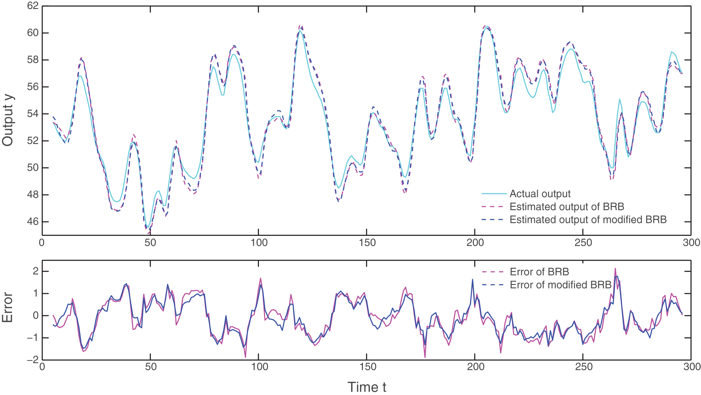
In the Box-Jenkins gas furnace experiment, the original dataset was recorded from a combustion process of a methane air mixture, and consists of 296 data pairs {(u (t) , y (t)) ; t = 1, ⋯ , 296}, where u (t) is the input gas flow rate, and y (t) is the observed output CO₂ concentration at the sampling time t. For the sake of comparative study, the same model from [5] is used. $y (t) = f (y (t - 1), u (t - 4))$ (28)

Thus there will be 292 input–output data pairs. We use the same parameter setting in [5] to construct the BRB model: five linguistic terms are used to define u (t), which are negative large (NL), negative small (NS), zero (Z), positive small (PS), and positive large (PL). These linguistic terms are associated with the following numerical referentialvalues: $A_{1}^{k} \in {NL, NS, Z, PS, PL} = {- 3, - 1.5, 0, 1.5, 3}$ Five linguistic terms are used to define y (t), which are very low (VL), low (L), medium (M), high (H), and very high (VH) and are associated with the following referential values: $A_{2}^{k} \in {VL, L, M, H, VH} = {45, 49, 53, 57, 61}$ The output y (t) is characterised by a belief distribution on {D₁, D₂, D₃, D₄, D₅} = {45, 49, 53, 57, 61} in each belief rule.

Given the above referential values, there are 25 referential combinations of the two antecedent inputs y (t - 1) and u (t - 4), leading to 25 belief rules in total. Table 2 lists the initial BRB parameters. There are 167 parameters in the original BRB model while only 67 parameters are remained in the modified one. The estimated outputs of the two BRB models with the initial parameters are plotted in Fig. 2. From the figure we can see that the two estimated output curves almost overlap, and there is little difference between their estimated errors. This is also reflected by the MSE between the actual output and the initial estimated outputs of them, which are 0.6223 and 0.6655, respectively. The result shows that using weighted averaging operator to replace ER approach in the BRB model would not cause obvious decline in its approximation capability.

Fig.2

BRB with initial parameters.

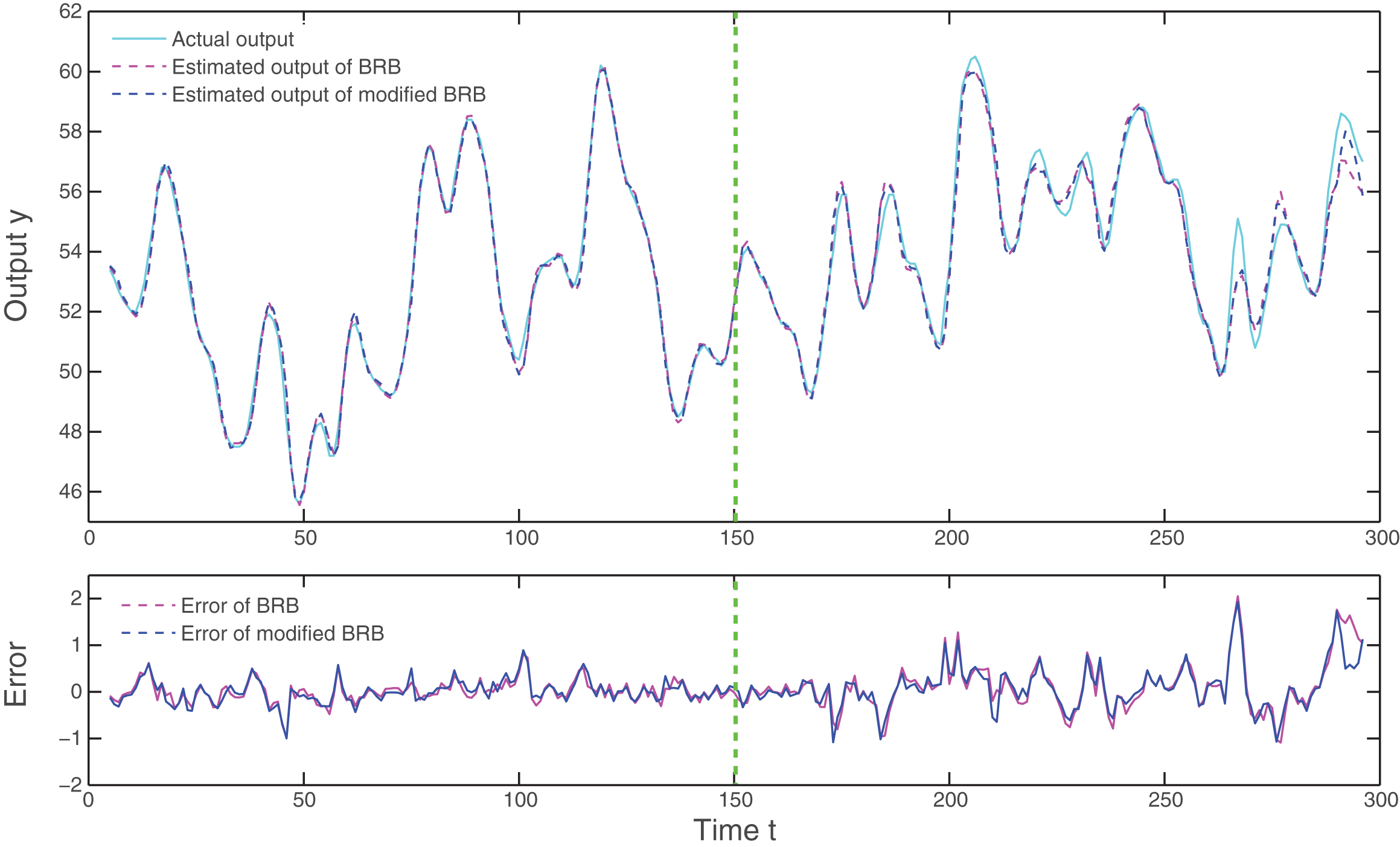
To train the BRB models, the first 150 data pairs are used as training set, and the remaining part of the dataset is used to test the training effect for validation purpose. Figure 3 shows the estimated outputs of the two trained BRB models for both training and testing datasets. It can be seen from the figure that the trained models have much better performance than the initial BRB models, and the modified BRB model is as good as the BRB model.

Fig.3

BRB with trained parameters.

Table 3 compares the original and modified BRB models with different numbers of referential values. We can see that the MSE is monotonically decreasing with the increase of the referential values, and that the modified BRB model achieves a comparative performance with BRB model in all cases. When it comes to the training time, the proposed method has a much better performance as shown in the last column. The training time of the modified BRB model is less than 1/10 of the original BRB model, and it increases slower as more referential values are used. Thus the modified BRB model is more suitable for complicated systems with a large scale belief rule base.

5.2 Two dimensional Sinc function

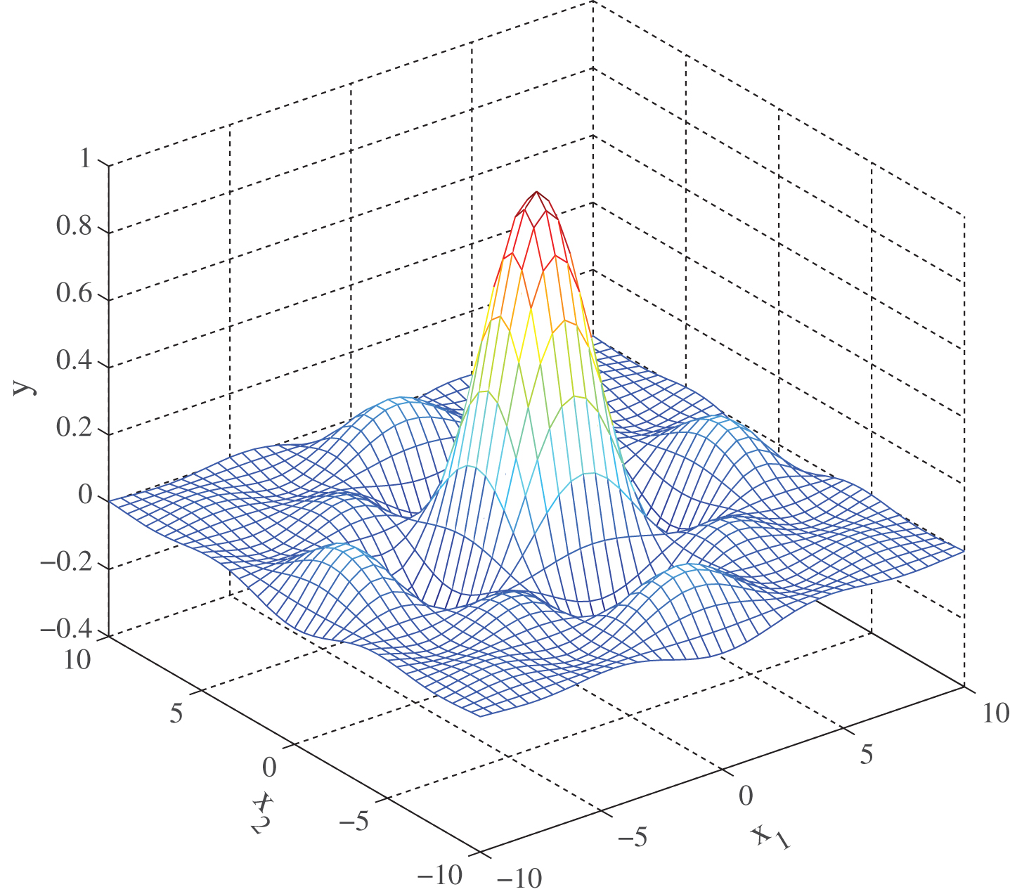
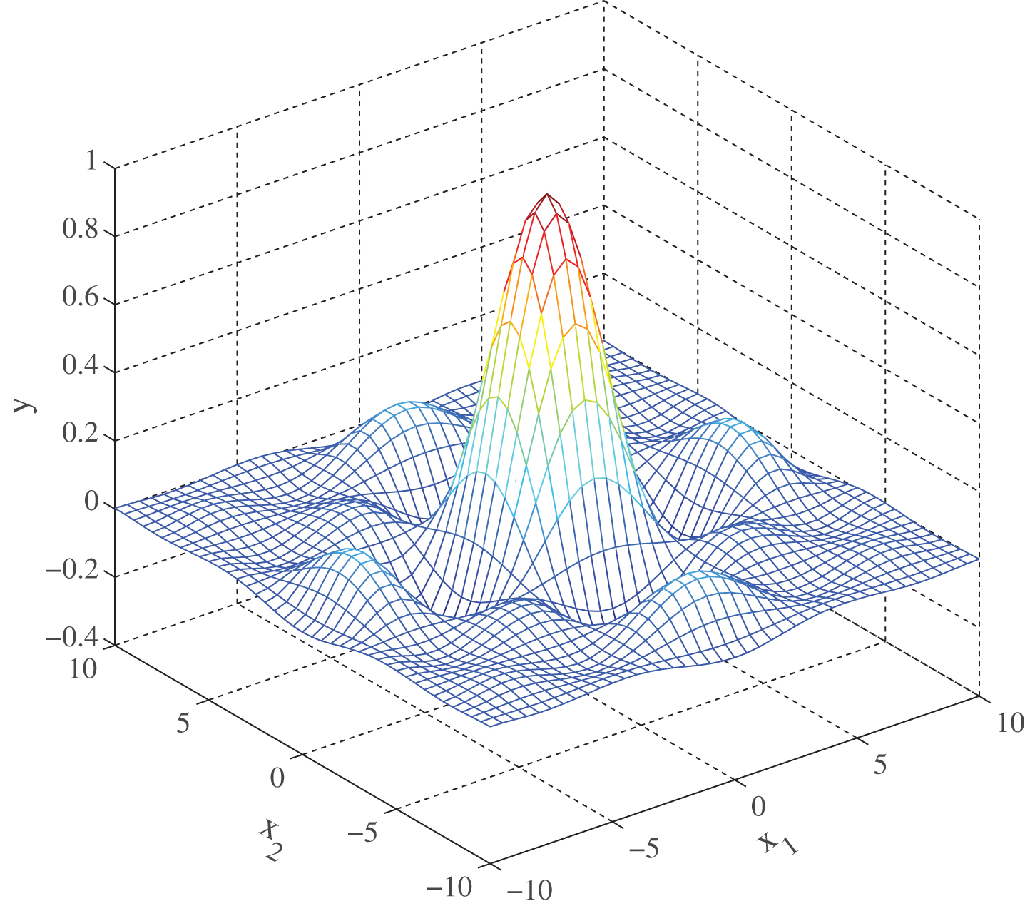
The data for this case study are generated from the following two-variable nonlinear function:

$y = \frac{sin x_{1}}{x_{1}} \times \frac{sin x_{2}}{x_{2}}$ (29)

Figure 4 shows its original surface. The training set consists of 1681 data points, arranged in a regular grid within the [–10,10]×[–10,10] domain. Initially, 9 referential values {–10, –7, –5, –2, 0, 2, 5, 7, 10} are used for both x₁ and x₂. Similarly to the first case study, a BRB model with 81 belief rules could be established. The initial values for θ_k and δ_i are all set to be 1, and v_k is arranged in a square matrix as explained in section 4.2 and initial values are defined as follows. $[v_{i, j}] = [\begin{matrix} 0 0 0 0 0 0 0 0 0 \\ 0 0 0 0 0 0 0 0 0 \\ 0 0 0 0 0 0 0 0 0 \\ 0 0 0 0 0 0 0 0 0 \\ 0 0 0 0 1 0 0 0 0 \\ 0 0 0 0 0 0 0 0 0 \\ 0 0 0 0 0 0 0 0 0 \\ 0 0 0 0 0 0 0 0 0 \\ 0 0 0 0 0 0 0 0 0 \end{matrix}]$

Using MSE as the objective function, a trained BRB model could be obtained. The trained values for v_k are listed in the following matrix.

$[v_{i, j}] = [\begin{matrix} - 0.0011 & - 0.0078 & 0.0122 & - 0.0186 & - 0.0449 & - 0.0187 & 0.0128 & - 0.0081 & - 0.0001 \\ - 0.0046 & 0.0239 & - 0.0398 & 0.0448 & 0.1497 & 0.0485 & - 0.0397 & 0.0240 & - 0.0052 \\ 0.0115 & - 0.0390 & 0.0629 & - 0.0649 & - 0.2245 & - 0.0688 & 0.0625 & - 0.0379 & 0.0129 \\ - 0.0184 & 0.0628 & - 0.0926 & 0.1937 & 0.4641 & 0.2022 & - 0.0908 & 0.0634 & - 0.0186 \\ - 0.0506 & 0.1616 & - 0.2477 & 0.3269 & 1.0000 & 0.3623 & - 0.2482 & 0.1648 & - 0.0517 \\ - 0.0184 & 0.0628 & - 0.0926 & 0.1937 & 0.4641 & 0.2022 & - 0.0908 & 0.0634 & - 0.0186 \\ 0.0115 & - 0.0390 & 0.0629 & - 0.0649 & - 0.2245 & - 0.0688 & 0.0625 & - 0.0379 & 0.0129 \\ - 0.0046 & 0.0239 & - 0.0398 & 0.0448 & 0.1497 & 0.0485 & - 0.0397 & 0.0240 & - 0.0052 \\ - 0.0011 & - 0.0078 & 0.0122 & - 0.0186 & - 0.0449 & - 0.0187 & 0.0128 & - 0.0081 & - 0.0001 \end{matrix}]$

Fig.4

Original surface of two dimensional Sinc function.

Fig.5

Estimated surface of modified BRB with 7 referential values.

In this matrix, we have v_i,3 > v_i,4 > v_i,5, v_i,5 < v_i,6 < v_i,7, i = 1, ⋯ , 9 and v_3,j > v_4,j > v_5,j, v_5,j < v_6,j < v_7,j, j = 1, ⋯ , 9. According to the attribute reduction approach introduced in section 4.2, two referential values could be reduced for both x₁ and x₂. Using the remaining parameter values as initial values and training it in the same way, another modified BRB model is established. The estimated surface is presented in Fig. 5.

Table 4 compares the results of the modified BRB models with some existing methods. The results obtained by our models are much better in terms of MSE. With the same number of rules, the modified BRB model with 7 referential values has a much smaller MSE than the 49-rule method provided by Evsukoff et al. Compared with the fuzzy model proposed by Rezaee, we also obtain a much smaller MSE, but more rules are used in our model. Note that the MSE decreases a lot after reducing the referential values from 9 to 7, but it would increase if referential values are further reduced to 6, this demonstrates the effectiveness of the proposed attribute reduction approach.

5.3 Case study 3

In this example [4, 26], there are a class of nonlinear functions G = {y = g_norm (x) + Δg (x)} with the nominal function g_norm (x) = cos(x) sin(x) and the uncertain part Δg (x) = γ cos(8x), 0 ⩽ γ ⩽ 0.2. The function from the class is defined in the input domain U = {x|-1 ⩽ x ⩽ 1} and the set of measured input is X = {x_t|x_t = 0.021t ; t = -47, - 46, ⋯ , 47}.

Firstly, we consider the approximation of the nominal function. The initial values for the modified BRB model are listed in Table 5. Training the model with the 95 input-output data pairs (x_t, g_norm (x_t)), trained values for A_j and v_k are obtained: A = { –0.9968, –0.7529, –0.5203, –0.3064, –0.1122, 0.1122, 0.3064, 0.5203, 0.7529, 0.9968} and [v_k]=[–0.4679, –0.5070, –0.4321, –0.2902, –0.1227, 0.1161, 0.2901, 0.4390, 0.5084, 0.4656]. It is easy to see that –0.5070 < –0.4321 < –0.2902 < –0.1227 <0.1161 <0.2901 <0.4390 <0.5084, thus we can at most reduce 6 referential values according to section 4.2. Set the new initial referential values for x as { –0.9968, –0.7529, 0.7529, 0.9968} and the values for v_k as [–0.4679, –0.5070, 0.5084, 0.4656], then train the model again. Figure 6 shows the estimated outputs of the modified BRB model with 10 and 4 referential values. We can see that the modified BRB can achieve an even better performance after reducing 6 referential values. In fact, the MSE decreases from 1.0 × 10^-5 to 2.7 × 10^-6 after 6 redundant referential values are abandoned. Generally, more referential values would lead to a higher approximation accuracy. However, one rule changes to another rule at each referential value, which may reduce the smoothness of the fitting curve as well as the overall approximation accuracy if many redundant referential values are used. This could be seen from the partial enlargement in Fig. 6.

Fig.6

Comparisons of modified BRB with different numbers of referential values.

In the following, we consider the nominal function combined with the uncertain part. In [26], eight triangular and equidistant membership functions are used for the first-order fuzzy model, thus generating 8 rules for upper bound and lower bound separately. Firstly, we also use 8 referential values for x, and the initial modified BRB model is listed in Table 6. The L_∞ norm in Equation (13) is used to train the model. The min-max problem can be solved as the nonlinear programming problem of minimizing σ subject to the following inequalities [4]: $y (t) - {\hat{y}}_{\min} (x (t)) \geq 0, t = 1, \dots, T$ (30a) $y (t) - {\hat{y}}_{\max} (x (t)) \leq 0, t = 1, \dots, T$ (30b) $y (t) - {\hat{y}}_{\min} (x (t)) \geq σ, t = 1, \dots, T$ (30c) $- y (t) + {\hat{y}}_{\max} (x (t)) \leq σ, t = 1, \dots, T$ (30d) $σ \geq 0$ (30e)

Figure 7 plots the estimated lower and upper bounds of the trained modified BRB model and the fuzzy model. We can see that the red curve covers all the uncertain outputs and gives a good estimation of the upper and lower bounds. Compared with the fuzzy model, it achieves smaller approximation errors in some local regions, but in regions near the nodes it has much bigger approximation errors. This is caused by lack of enough referential values.

Fig.7

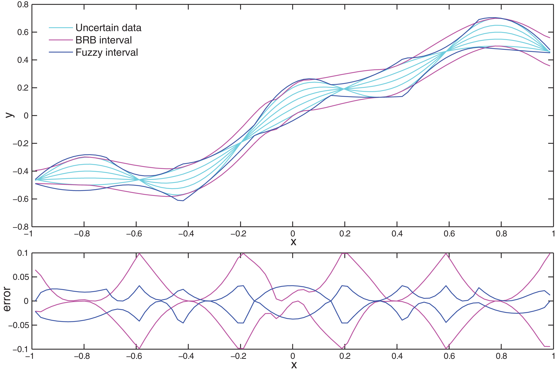
Comparison of modified BRB(8 ref.) and fuzzy model.

Fig.8

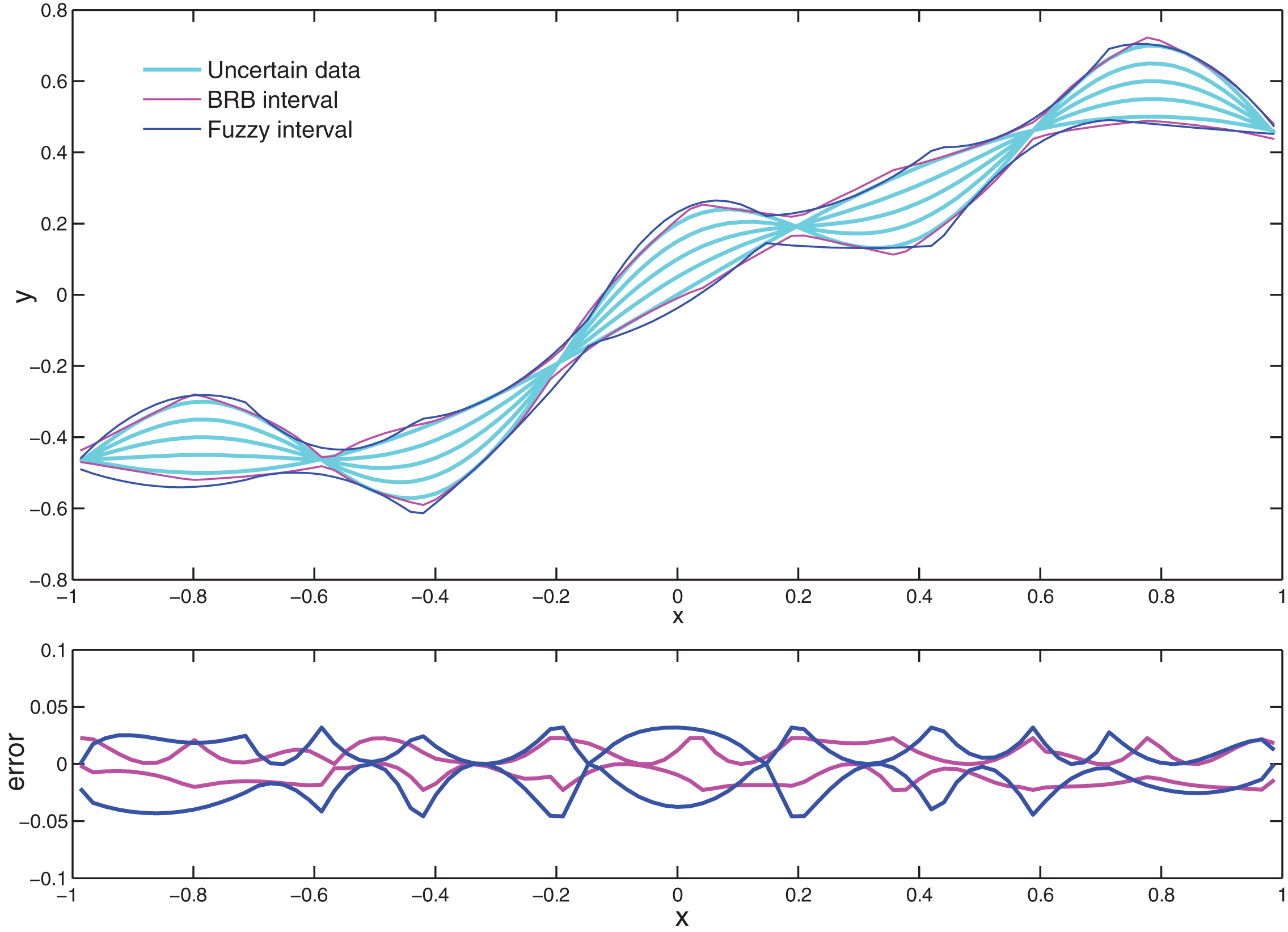
Comparison of modified BRB(11 ref.) and fuzzy model.

In the fuzzy model, the lower and upper bounds are estimated by independent fuzzy models. Though 8 membership functions are used, there are 16 fuzzy rules in total. In the modified BRB model, both bounds are estimated by one model and there are only 8 belief rules. If we increase the number of belief rules to 16, a better performance could be obtained. In fact, when 11 belief rules are used, the modified BRB model would outperform the first-order fuzzy model, as shown in Fig. 8. It is easy to see that the modified BRB model obtains a better interval estimation.

In this case study, we can also use two independent modified BRB models with complete belief rules for the upper and lower bounds respectively, just like the fuzzy model. However, one BRB model with incomplete belief rules is more preferred in the uncertain case since it has a simpler training process with comparative approximation results.

6 Conclusion

BRB models are capable of modelling uncertain nonlinear systems. In this paper, weighted averaging operator is applied in the inference process in place of ER approach to aggregate all activated belief rules. This substitution together with some algebraic transformations generates the modified BRB model, which has a simpler model structure. Compared with the original BRB model, it reduces model parameters significantly and cut down the time for training rapidly. Besides, its universal approximation capability is guaranteed by the Stone–Weierstrass theorem. Based on the special structure of the modified BRB model, an approach for reducing possibly redundant referential values is put forward to achieve a tradeoff between approximation accuracy and model complexity.

Comparisons between the modified BRB model and the original one show that they have comparative performance though the former one has a much simpler structure. The performance of the modified BRB model with the attribute reduction approach is further validated by two well known case studies. It should be noted that the method is not proposed to replace the existing methods, but to improve the efficiency of the original BRB model and provides an alternative to the uncertain nonlinear systems identification problem.

The proposed attribute reduction approach is designed for point estimate problems. In the case of interval estimate, belief rules are incomplete with different degrees of uncertainty. Both consequents and degrees of uncertainty should be considered when reducing referential values, which will be researched in our future work.

References

Calzada

, Liu

, Wang

and Kashyap

, A new dynamic rule activation method for extended belief rule-based systems, IEEE Transactions on Knowledge and Data Engineering 27 (2015), 880–894.

Campi

M.C.

and Weyer

, Guaranteed non-asymptotic confidence regions in system identification, Automatica 41 (2005), 1751–1764.

Chang

, Zhou

, Jiang

, Li

and Zhang

, Structure learning for belief rule base expert system: A comparative study, Knowledge-Based Systems 39 (2013), 159–172.

Chen

Y.W.

, Yang

J.B.

, Pan

C.C.

, Xu

D.L.

and Zhou

Z.J.

, Identification of uncertain nonlinear systems: Constructing belief rulebased models, Knowledge-Based Systems 73 (2015), 124–133.

Chen

Y.W.

, Yang

J.B.

, Xu

D.L.

and Yang

S.L.

, On the inference and approximation properties of belief rule based systems, Information Sciences 234 (2013), 121–135.

Chen

Y.W.

, Yang

J.B.

, Xu

D.L.

, Zhou

Z.J.

and Tang

D.W.

, Inference analysis and adaptive training for belief rule based systems, Expert Systems with Applications 38 (2011), 12845–12860.

Cheney

E.W.

, AMS Chelsea Publishing, Introduction to Approximation Theory 1998.

Deng

, Shi

, Zhu

and Liu

, Combining belief functions based on distance of evidence, Decision Support Systems 38 (2004), 489–493.

Denœux

, Younes

and Abdallah

, Representing uncertainty on set-valued variables using belief functions, Artificial Intelligence 174 (2010), 479–499.

10.

Evsukoff

, Branco

A.C.

and Galichet

, Structure identification and parameter optimization for non-linear fuzzy modeling, Fuzzy Sets and Systems 132 (2002), 173–188.

11.

, Huhns

and Yang

, A consensus framework for multiple attribute group decision analysis in an evidential reasoning context, Information Fusion 17 (2014), 22–35.

12.

González-Olvera

and Tang

, Black-box identification of a class of nonlinear systems by a recurrent neurofuzzy network, IEEE Transactions on Neural Networks 21 (2010), 672–679.

13.

Hayes-Roth

, Rule-based systems, Communications of the ACM 28 (1985), 921–932.

14.

Khosravi

, Nahavandi

, Creighton

and Atiya

A.F.

, Lower upper bound estimation method for construction of neural network-based prediction intervals, IEEE Transactions on Neural Networks 22 (2011), 337–346.

15.

Lawry

and Tang

, Uncertainty modelling for vague concepts: A prototype theory approach, Artificial Intelligence 173 (2009), 1539–1558.

16.

Ligeza

, Principles of Verification of Rule-Based Systems, Springer, 2006.

17.

Murphy

C.K.

, Combining belief functions when evidence conflicts, Decision Support Systems 29 (2000), 1–9.

18.

Nelles

, Nonlinear system identification: From classical approaches to neural networks and fuzzy models, Berlin, Heidelberg: Springer-Verlag, 2001.

19.

Parmigiani

and Inoue

, Decision theory: Principles and approaches, John Wiley & Sons, 2009.

20.

Rezaee

and Zarandi

M.F.

, Data-driven fuzzy modeling for Takagi-Sugeno-Kang fuzzy system, Information Sciences 180 (2010), 241–255.

21.

Senthilkumar

and Mahanta

, Identification of uncertain nonlinear systems for robust fuzzy control, ISA Transactions 49 (2010), 27–38.

22.

Shafer

G.A.

, A mathematical theory of evidence, Princeton University Press, 1976.

23.

X.S.

, Hu

C.H.

, Yang

J.B.

and Zhou

Z.J.

, A new prediction model based on belief rule base for system’s behavior prediction, IEEE Transactions on Fuzzy Systems 19 (2011), 636–651.

24.

Sjöberg

, Zhang

, Ljung

, Benveniste

, Delyon

, et al., Nonlinear black-box modeling in system identification: A unified overview, Automatica 31 (1995), 1691–1724.

25.

Škrjanc

, Blažič

and Agamennoni

, Identification of dynamical systems with a robust interval fuzzy model, Automatica 41 (2005), 327–332.

26.

Škrjanc

, Blažič

and Agamennoni

, Interval fuzzy model identification using L_∞-norm, IEEE Transactions on Fuzzy Systems 13 (2005), 561–568.

27.

Uncu

Ö.

, Türkşen

Î.B.

, Discrete interval type 2 fuzzy system models using uncertainty in learning parameters, IEEE Transactions on Fuzzy Systems 15 (2007), 90–106.

28.

Wang

, Su

Z.G.

, Rezaee

and Wang

P.H.

, Constructing T-S fuzzy model from imprecise and uncertain knowledge represented as fuzzy belief functions, Neurocomputing 166 (2015), 319–366.

29.

Wang

Y.M.

, Yang

L.H.

, Chang

L.L.

and Fu

Y.G.

, Rough set method for rule reduction in belief rule base, Control and Decision 29 (2011), 1944–1950.

30.

D.L.

, Liu

, Yang

J.B.

, Liu

G.P.

, Wang

, Jenkinson

and Ren

, Inference and learning methodology of belief-rule-based expert system for pipeline leak detection, Expert Systems with Applications 32 (2007), 103–113.

31.

Yang

J.B.

, Liu

, Wang

, Sii

H.S.

and Wang

H.W.

, Belief rule-base inference methodology using the evidential reasoning approach - RIMER, IEEE Transactions on Systems, Man and Cybernetics, Part A: Systems and Humans 36 (2006), 266–285.

32.

Yang

J.B.

and Xu

D.L.

, On the evidential reasoning algorithm for multiple attribute decision analysis under uncertainty, IEEE Transactions on Systems, Man and Cybernetics, Part A: Systems and Humans 32 (2002), 289–304.

33.

Zhou

Z.J.

, Hu

C.H.

, Yang

J.B.

, Xu

D.L.

, Chen

M.Y.

and Zhou

D.H.

, A sequential learning algorithm for online constructing belief-rule-based systems, Expert Systems with Applications 37 (2010), 1790–1799.