An edge-based finite element method for 3D marine controlled-source electromagnetic forward modeling with a new type of second-order tetrahedral edge element

Abstract

This paper presents a second order edge-based finite element method based on a new type of second order edge element for numerical modeling of 3D controlled source electromagnetic data in an anisotropic conductive medium. We adopt the anomalous potential field formulation to avoid the effect of source’s singularity. The computational domain was subdivided into unstructured tetrahedral elements. The sparse linear system was solved using the Induced dimensional reduction (IDR(s)) method with an incomplete LU preconditioner. We have applied the developed algorithm to compute a typical MCSEM response over several 3D models, we compare the numerical results from our method and FEM solution based on conventional first and second order element. The results of comparison shown that our algorithm can significantly reduce the computation cost without loss to much accuracy.

Keywords

Marine controlled sources electromagnetic method second order element edge-based finite element method anisotropic modeling

1. Introduction

In recent twenty years, the marine controlled-sources electromagnetic method (MCSEM) has become an important exploration tool, which is widely used in the exploration of hydrocarbon resources, deep geological structure and so on. To achieve the purpose of quantitative imaging of complex subsurface resistivity distributions and extracting as much information as possible from survey data, it is necessary to improve the accuracy and efficiency of the 3D forward modeling of the marine source controlled electromagnetic method. There are some conventional approaches for numerically modelling EM problems: the integral equation (IE) method [1, 2, 3, 4], finite difference (FD) method [5, 6], finite volume (FV) method [7, 8, 9] and finite element (FE) method [10, 11, 12, 13, 14, 15, 16]. The IE method only need to require the discretization for the anomalous domain, which typically give rise to fully populated matrices [17, 18]. This method is more suitable for simple model and the store requirement and computation time will be obviously increases with the increasing of model complexity. Finite Difference Method is the simplest in concept, and can be easily implemented [19]. However, it can only be used in rectangular brick to discretize the modeling domain. Therefore, the Finite Difference Method is not suitable for modeling the EM response in complex geoelectrical structures [14]. The FV method approximates the field at a nodal point in space through integrating the relevant PDEs over an averaging volume surrounding that point [8, 9]. Compare to the above-mentioned methods, the FE method can easy to use the unstructured mesh to discrete the modeling domain, this advantage makes it more suitable modeling the response of complex models. What is more, it can locally refine the interest region and coarsen the area near the domain boundary [12, 13]. Therefore, the efficiency of mesh generation can be improved effectively.

There are two types of finite element method for CSEM modeling due to its geometric flexibility: nodal-base finite element method and edge-based finite element method. The conventional node-based FE suffers from spurious solutions since the divergence free condition in source free region and the tangential field continuity is not imposed [20, 21]. Compare to the conventional node-based FE method, the edge-based FE method just overcomes this obstacle and attracts many researcher’s attention and has been widely used for solving electromagnetic field problems [22]. However, these elements are built in first order. In order to further increase the accuracy of edge elements, we can use higher order edge elements to approximate. However, such elements bring a large increase in the number of variables, many of them being redundant. This will significantly increase the computational time. Therefore, how to improve the accuracy of calculation without obvious increase of computational cost is crucial.

As far as the stability of the solution is concerned, the vector Helmholtz equation, expressed solely in terms of the electric filed or magnetic field, is a partial differential equation (PDE) of second order. Solving this PDE for a situation where the EM fields are discretized using linear basis functions, and where very low frequencies are used, is not efficient [23]. However, the above problems can be avoided by using the potential in forward modeling EM problem. There are some studies using potential in 3D forward modeling of geophysical EM problems [24, 25]. Furthermore, the potential field FE approximation for wave and eddy current problems in electrical engineering [26, 27].

In this paper, we formulate the 3D marine CSEM problem using a new type second-order edge element in the anisotropic medium. In order to avoid the sources singularity, we apply the anomalous vector and scalar potential field formation to solve the Maxwell’s equations. In order to simulate the bathymetry effect, we use tetrahedral elements to discrete modeling domain. The sparse finite element system of equations is solved using an IDR(s) method with the ILU preconditioner. We validate our algorithm by several models and compare the numerical results from our method and conventional 1 ${}^{\text{st}}$ and 2 ${}^{\text{nd}}$ order edge-elements based finite element solutions.

2. Theory

2.1 Governing equations

Without loss of generality, the low frequency electromagnetic field, considered in geophysical application, satisfies the following Maxwell’s equations [17]:

$\displaystyle\nabla\times\bm{E}=i\omega\mu_{0}\bm{H}$ (1) $\displaystyle\nabla\times\bm{H}=J_{s}+\bar{\sigma}\bm{E}$ (2)

Where $\mu_{0}$ denotes the free space magnetic permeability. $\omega$ denotes the angular frequency. $J_{s}$ denotes the distribution of source current. $\bar{\sigma}$ denotes the conductivity tensor which is defined as follows:

$\displaystyle\bar{\bm{\sigma}}=\left({\begin{array}[]{*{20}c}\sigma_{x}&0&0\\ 0&\sigma_{y}&0\\ 0&0&\sigma_{z}\\ \end{array}}\right)$ (3)

According to the definition of the Coulomb vector and scalar potential, the electromagnetic fields $E$ and $H$ can be written as follows [10]:

$\displaystyle\bm{H}=\frac{1}{\mu_{0}}\nabla\times\bm{A}$ (4) $\displaystyle\bm{E}=i\omega\left(\bm{A}+\nabla\Psi\right)$ (5)

Substituting Eqs (4) and (5) into Eqs (2) and (3), and the following Helmholtz equation can be obtained:

$\displaystyle\nabla\times\nabla\times\bm{A}-i\omega\mu_{0}\bar{\bm{\sigma}}% \left(\bm{A}+\nabla\Psi\right)=\mu_{0}\bm{J}_{\bm{s}}$ (6) $\displaystyle\nabla\cdot\left[i\omega\mu_{0}\bar{\bm{\sigma}}\left(\bm{A}+% \nabla\Psi\right)\right]=-\nabla\cdot\left(\mu_{0}\bm{J}_{\bm{s}}\right)$ (7)

In order to avoid the singularities of sources. We apply the anomalous field formulation on 3D marine CSEM modeling. In the anomalous field formulation of diffusive EM field problem. The total conductivity tensor is decomposed into background conductivity tensor and the anomalous conductivity tensor.

$\displaystyle\bar{\bm{\sigma}}=\Delta\bar{\bm{\sigma}}+\bar{\bm{\sigma}}_{\bm{% p}}$ (8)

Similarly, the total Coulomb vector and scalar potential can be decomposed into background and anomalous fields.

$\displaystyle\bm{A}=\bm{A}_{\bm{p}}+\bm{A}_{\bm{s}}$ (9) $\displaystyle\Psi=\Psi_{\bm{p}}+\Psi_{\bm{s}}$ (10)

Where $\bm{A}_{\bm{p}}$ is the primary vector potential, $\Psi_{\bm{p}}$ is the primary scalar potential, $\bm{A}_{\bm{s}}$ is the anomalous vector potential. $\Psi_{\bm{s}}$ is the anomalous scalar potential.

Substituting Eqs (9) and (10) into the Eqs (6) and (7). The Helmholtz equation for the anomalous potential field can be obtained as follow:

$\displaystyle\nabla\times\nabla\times\bm{A}_{\bm{s}}-i\omega\mu_{0}\bar{\bm{% \sigma}}\left(\bm{A}_{\bm{s}}+\nabla\Psi_{s}\right)=i\omega\mu_{0}\Delta\bar{% \bm{\sigma}}\left(\bm{A}_{p}+\nabla\Psi_{p}\right)$ (11) $\displaystyle\nabla\cdot\left[i\omega\mu_{0}\bar{\bm{\sigma}}\left(\bm{A}_{\bm% {s}}+\nabla\Psi_{s}\right)\right]=-\nabla\cdot\left[i\omega\mu_{0}\Delta\bar{% \bm{\sigma}}\left(\bm{A}_{p}+\nabla\Psi_{p}\right)\right]$ (12)

From Eqs (11) and (12), one can see that the source term for this equation is the primary potential field, which can be computed analytically for a full-space and half-space background conductivity. For a general layered earth model, the primary potential field can be computed semi-analytically by using a digital filter algorithm to calculate Hankel transforms.

3. Second-order edge-based element

Similar to the conventional node-based finite element method, the edge-based finite element method can discretize modeling domain using rectangular, tetrahedron, hexahedron or other complex elements [21, 22]. In order to simulate complex seabed topography. In this study, we use the tetrahedron elements to discretize modeling domain. Besides, we apply second-order Edge Element approximation to improve the solution accuracy. In this section, we will introduce a new second-order Edge Element and compare to conventional second-order edge element. In this paper, geometrical edge of a finite element is called side and the location related to a vector variable is called edge. In the case of second-order elements, sides and edges are not the same but there are two edges on each side.

Figure 1.

Conventional second-order tetrahedral elements.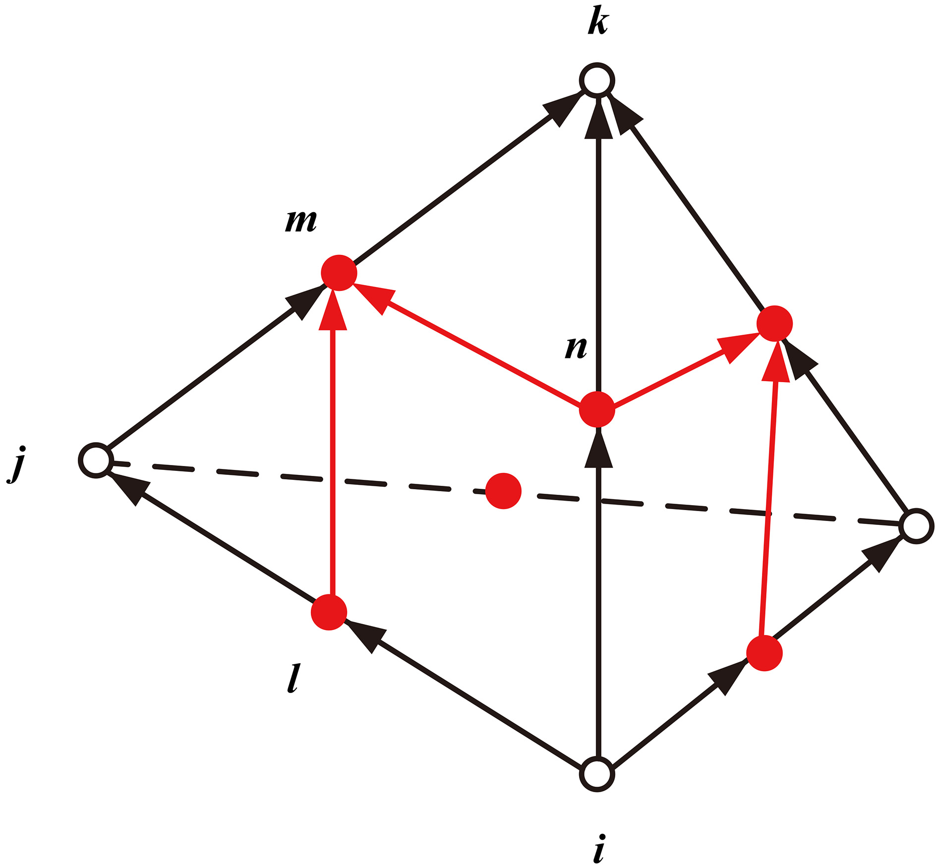

3.1 Conventional second-order edge element

Figure 1 shows the conventional second-order edge element [28]. Form the Fig. 1 one can find that there are 10 nodes and 20 edges in the conventional second-order edge element. In general, there should be 10 nodes and 24 edges in the second-order edge element. However, since the curls of edge shape function within an edge element are linearly dependent. So, some edge variables become redundant. We can reduce them by using tree gauging method. In the potential edge-element FE schemes, the vector and scalar potentials are defined along the edges and at the nodes of the tetrahedral element, respectively. The edge shape functions $\bm{N}$ and node shape function $N$ of element can be defined as follow:

$\displaystyle\bm{N}_{\bm{il}}=\left(4\lambda_{i}-1\right)\left(\lambda_{i}% \nabla\lambda_{j}-\lambda_{j}\nabla\lambda_{i}\right)$ (13) $\displaystyle\bm{N}_{\bm{nm}}=4\lambda_{k}\left(\lambda_{i}\nabla\lambda_{j}-% \lambda_{j}\nabla\lambda_{i}\right)$ (14) $\displaystyle N_{\bm{i}}=\left(2\lambda_{i}-1\right)\lambda_{i}$ (15) $\displaystyle N_{\bm{l}}=4\lambda_{i}\lambda_{j}$ (16)

Where ${\bm{\lambda}}=\left({\lambda}_{1},{\lambda}_{2},{\lambda}_{3},{\lambda}_{4}\right)$ denote the barycentric coordinates of element. $i, j, k$ denote the nodes at the vertices. $m, n, l$ denote the mid-nodes on the edges $-j$ , $j-k$ , $k-i$ , respectively. $\bm{N}_{\bm{il}}$ denotes the shape function on the sides (black arrow vector). $\bm{N}_{\bm{nm}}$ is the shape function on the faces (red arrow vector). $N_{\bm{i}}$ and $N_{\bm{l}}$ are the shape function of nodes at the vertices and mid-nodes on the edges, respectively.

The shape function of all faces has the following relation:

$\displaystyle\sum_{nm}N_{nm}=0$ (17)

From the Eq. (17), we can find that one of the shape function of faces is redundant. Therefore, we can eliminate the corresponding edge variable, then the computation cost can be significantly reduced. In next section, we will discussion new method to eliminate some redundant edge variable.

Figure 2.

Unification of two edges. (a) Two edges on the side. (b) Unified edge.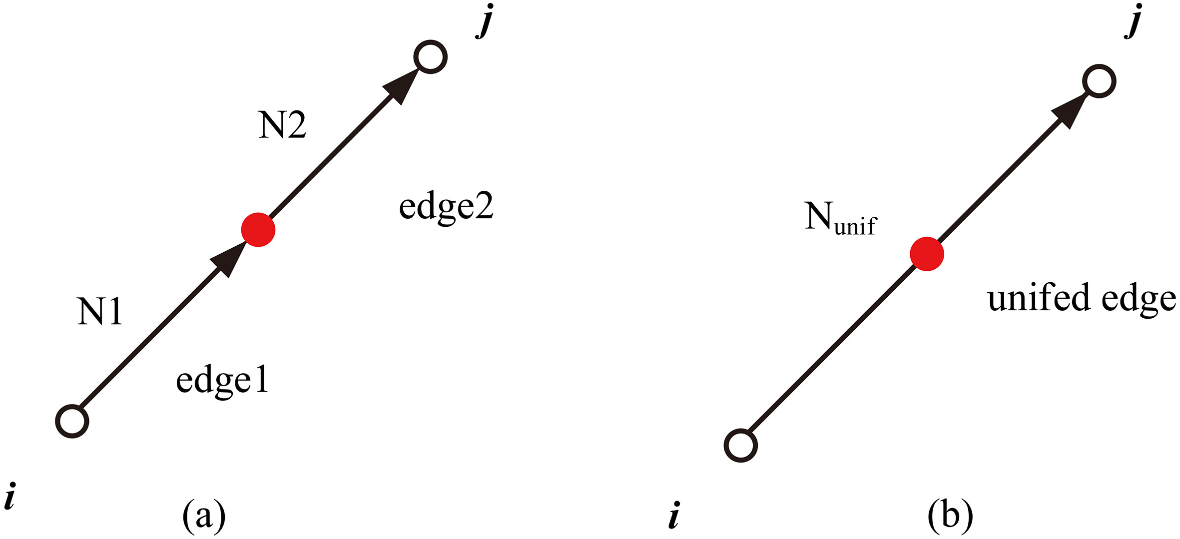

3.2 New type of second-order edge element

Without loss of generality, we first consider a one side of conventional second-order edge element as shown in the Fig. 1. There are two edges on the sides of second-order edge element as shown in the Fig. 2a. We named them edge1 and edge2, respectively. We assume the shape function of edge1 and edge2 is N1 and N2, respectively. And the corresponding edge variables of these two edges is A1 and A2, respectively. In this case, the one of A1 and A2 can be eliminated, therefore we decide to eliminated A2 as the redundant edge variable and consider A1 $=$ A2. We assume the ${A}_{\textit{side}}$ as the contribution of the two edges to the interpolation of the vector potential within the element. Then, we can obtain the equation as follows:

$\displaystyle{A}_{\textit{side}}=N_{1}A_{1}+N_{2}A_{2}=(N_{1}+N_{2})A_{1}$ (18)

We let ${A}_{\textit{umif}}$ to be the line integral of $A$ along the side. Considering the follow orthogonal properties:

$\displaystyle\int_{\textit{eKL}}N_{IL}ds=\delta_{\left(IL\right)\left(KL\right)}$ (19)

Where $d s$ denotes the line element vector along edge eKL, $\delta_{\left(IL\right)\left(KL\right)}$ denotes the Kronecker delta. Then ${A}_{\textit{umif}}$ can be expressed as follows:

$\displaystyle{A}_{\textit{umif}}=\int_{\textit{edge1}}\textit{Ads}+\int_{% \textit{edge2}}\textit{Ads}=A_{1}+A_{2}=2A_{1}$ (20)

Then the Eq. (18) can be rewritten as follows:

$\displaystyle{A}_{\textit{side}}=(N_{1}+N_{2})A_{1}=\left(N_{1}+N_{2}\right)% \frac{{A}_{\textit{umif}}}{2}=N_{\textit{umif}}{A}_{\textit{umif}}$ (21)

Where $N_{\textit{umif}}=\frac{\left(N_{1}+N_{2}\right)}{2}$ is the new shape function of edge as shown in the Fig. 2b. According to Eq. (12), we final obtain the $N_{\textit{umif}}$ as follows:

$\displaystyle N_{\textit{umif}}=N_{IL}=\left(2(\lambda_{i}+\lambda_{j})-1% \right)\left({\lambda}_{i}{\nabla}{\lambda}_{j}-{\lambda}_{j}{\nabla}{\lambda}% _{i}\right)$ (22)

And the shape functions of the edges on the faces and the scalar shape functions is the same as the conventional second-order edge element. Then, we can obtain a new second-order edge element with 10 nodes and 14 edges as shown in the Fig. 3. Compare to the conventional second-order edge element as shown in the Fig. 1. The number of unknowns of new type second-order element is obviously less than those of the conventional second-order edge-element. Therefore, the computation cost can be obviously reduced.

Figure 3.

The proposed second order element.

4. Edge-based finite element analyses

Using the Galerkin’s method, the weak form of Eq. (11) can be written as:

$\displaystyle R=\nabla\times\nabla\times\bm{A}_{\bm{s}}-i\omega\mu_{0}\bar{\bm% {\sigma}}\left(\bm{A}_{\bm{s}}+\nabla\Psi_{s}\right)-i\omega\mu_{0}{\Delta}% \bar{\bm{\sigma}}\left(\bm{A}_{p}+{\nabla}\Psi_{p}\right)$ (23)

The inner product of the vector residual in Eqs (23) and (24) with a weight function $W$ is then equated to zero:

$\displaystyle\int_{\Omega}W\cdot Rd{\Omega=0}$ (24)

Substituting Eq. (23) into the Eq. (24) and integrating the first term

$\displaystyle\int_{\Omega}\left(\nabla\times\bm{W}\right)\cdot\left(\nabla% \times\bm{A}_{\bm{s}}\right)d{\Omega}-\int_{s}\bm{W}\times\nabla\times\bm{A}_{% \bm{s}}d\bm{s}-\int_{\Omega}i\omega\mu_{0}\bar{\bm{\sigma}}\bm{W}\cdot\bm{A}_{% \bm{s}}d{\Omega}$ $\displaystyle\quad-\int_{\Omega}i\omega\mu_{0}\bm{W}\cdot\nabla\Psi_{s}d\Omega% =\int_{\Omega}i\omega\mu_{0}{\Delta}\bar{\bm{\sigma}}\bm{W}\cdot\bm{A}_{\bm{p}% }d\Omega+\int_{\Omega}i\omega\mu_{0}{\Delta}\bar{\bm{\sigma}}\bm{W}\cdot{% \nabla}\Psi_{p}d{\Omega}$ (25)

By considering the continuity of the inner boundary and also the field is prescribed in the outer boundary, the surface integral in Eq. (4) can be ignored, then Eq. (4) can be rewritten as:

$\displaystyle\int_{\Omega}\left(\nabla\times\bm{W}\right)\cdot\left(\nabla% \times\bm{A}_{\bm{s}}\right)d{\Omega}-\int_{\Omega}i\omega\mu_{0}\bar{\bm{% \sigma}}\bm{W}\cdot\bm{A}_{\bm{s}}d{\Omega}-\int_{\Omega}i\omega\mu_{0}\bm{W}% \cdot\nabla\Psi_{s}d{\Omega}=\int_{\Omega}i\omega\mu_{0}{\Delta}\bar{\bm{% \sigma}}\bm{W}\cdot\bm{A}_{\bm{p}}d{\Omega}+\int_{\Omega}i\omega\mu_{0}{\Delta% }\bar{\bm{\sigma}}\bm{W}\cdot{\nabla}\Psi_{p}d{\Omega}$ (26)

Similar to vector residual of Eq. (11), the scalar residual of Eq. (11) is also minimized by calculating the product of the scalar residual $r$ with a scalar weight function $v$ and then integrating over the physical domain of the problem:

$\displaystyle\int_{\Omega}v\cdot rd\Omega=0$ (27)

Where

$\displaystyle r=\nabla\cdot\left[i\omega\mu_{0}\bar{\bm{\sigma}}\left(\bm{A}_{% \bm{s}}+\nabla\Psi_{s}\right)\right]+\nabla\cdot\left[i\omega\mu_{0}{\Delta}% \bar{\bm{\sigma}}\left(\bm{A}_{p}+\nabla\Psi_{p}\right)\right]$ (28)

By substituting the residual term Eq. (28) into Eq. (27) and applying integration by parts to the integral on the right side, the following equation is derived:

$\displaystyle\int_{\Omega}i\omega\mu_{0}\bar{\bm{\sigma}}\nabla v\cdot\bm{A}_{% \bm{s}}d\Omega-\int_{s}i\omega\mu_{0}v\bm{A}_{\bm{s}}\cdot\bm{nds}+\int_{% \Omega}i\omega\mu_{0}\bar{\bm{\sigma}}\nabla v\cdot\nabla\Psi_{s}d\Omega-\int_% {s}i\omega\mu_{0}v\nabla\Psi_{s}\cdot\bm{nds}=-\int_{\Omega}i\omega\mu_{0}% \Delta\bar{\bm{\sigma}}\nabla v\cdot\bm{A}_{\bm{p}}d{\Omega}+\int_{s}i\omega% \mu_{0}v\bm{A}_{\bm{p}}\cdot\bm{nds}-\int_{\Omega}i\omega\mu_{0}\Delta\bar{\bm% {\sigma}}\nabla v\cdot\nabla\Psi_{p}d{\Omega}+\int_{s}i\omega\mu_{0}v\nabla% \Psi_{p}\cdot\bm{nds}$ (29)

By considering the continuity of the inner boundary and also the field is prescribed in the outer boundary, the surface integral in Eq. (29) also can be ignored, then Eq. (29) can be rewritten as:

$\displaystyle\int_{\Omega}i\omega\mu_{0}\bar{\bm{\sigma}}\nabla v\cdot\bm{A}_{% \bm{s}}d{\Omega}+\int_{\Omega}i\omega\mu_{0}\bar{\bm{\sigma}}\nabla v\cdot% \nabla\Psi_{s}d{\Omega}=-\int_{\Omega}i\omega\mu_{0}\Delta\bar{\bm{\sigma}}% \nabla v\cdot\bm{A}_{\bm{p}}d{\Omega}-\int_{\Omega}i\omega\mu_{0}\Delta\bar{% \bm{\sigma}}\nabla v\cdot\nabla\Psi_{p}d{\Omega}$ (30)

In order to solve the Eqs (26) and (30), we first use the tetrahedron elements to discretize modeling domain, and apply the new type second-Order Edge Element presented in this paper to improve the solution accuracy. Within each element, the approximated vector and scalar potentials are expressed by using the vector and scaler basis functions:

$\displaystyle\bm{A}_{s}=\sum\limits_{IJ}\bm{N}_{IJ}\bm{A}_{s,IJ}$ (31) $\displaystyle\Psi_{s}=\sum\limits_{I}N_{I}\Psi_{s_{I}}$ (32) $\displaystyle\bm{A}_{p}=\sum\limits_{IJ}\bm{N}_{IJ}\bm{A}_{p,IJ}$ (33) $\displaystyle\Psi_{p}=\sum\limits_{I}N_{I}\Psi_{p_{I}}$ (34)

Where $\bm{N}_{IJ}$ and $N_{IJ}$ are vector and scalar basis function, respectively, and the parameters $\bm{A}_{s,IJ}$ and $\Psi_{p_{I}}$ are the unknown coefficients to be determined. Where ${I}$ and $J$ are node indices, and $I J$ denotes the direction of the edge from node $I$ to node $J$ .

The Galerkin version of the method of weighted residuals, in which the weighting function is chosen to be equal to the basis function, that is $\bm{W}=\bm{N}$ for the vector and $v=N$ for the scalar weight functions. By substituting the Eqs (31)–(34) in to the Eqs (26) and (30), we can find the discretized form of Eq. (26) for each element:

$\displaystyle\sum\limits_{j=1}^{N_{\textit{edges}}}A_{s,j}\int_{\Omega}\left({% \nabla}\times\bm{N}_{\bm{i}}\right)\cdot\left({\nabla}\times\bm{N}_{\bm{j}}% \right)d{\Omega}-iw\mu_{0}\bar{\sigma}\sum\limits_{j=1}^{N_{\textit{edges}}}A_% {s,j}\int_{\Omega}\bm{N}_{\bm{i}}\cdot\bm{N}_{\bm{j}}d{\Omega}-iw\mu_{0}\bar{% \sigma}\sum\limits_{k=1}^{N_{\textit{nodes}}}\Psi_{s,k}\int_{\Omega}\bm{N}_{% \bm{i}}{\cdot}{\nabla}N_{k}d{\Omega}=iw\mu_{0}\Delta\bar{\sigma}\sum\limits_{j% =1}^{N_{\textit{edges}}}A_{P,j}\int_{\Omega}\bm{N}_{\bm{i}}\cdot\bm{N}_{\bm{j}% }d\Omega+iw\mu_{0}\Delta\bar{\sigma}\sum\limits_{k=1}^{N_{\textit{nodes}}}\Psi% _{p,k}\int_{\Omega}\bm{N}_{\bm{i}}\cdot{\nabla}N_{k}d{\Omega}i\omega\mu_{0}% \sum\limits_{j=1}^{N_{\textit{edges}}}A_{s,j}\int_{\Omega}{\nabla}N_{l}\cdot% \left(\bar{\bm{\sigma}}\bm{N}_{\bm{j}}\right)d\Omega+i\omega\mu_{0}\sum\limits% _{k=1}^{N_{\textit{nodes}}}\Psi_{s,k}\int_{\Omega}{\nabla}N_{l}\cdot\left(\bar% {\bm{\sigma}}{\nabla}N_{k}\right)d\Omega$ (35) $\displaystyle=-i\omega\mu_{0}\sum\limits_{j=1}^{N_{\textit{edges}}}A_{p,j}\int% _{\Omega}{\nabla}N_{l}\cdot\left(\Delta\bar{\bm{\sigma}}\bm{N}_{\bm{j}}\right)% d\Omega-i\omega\mu_{0}\sum\limits_{k=1}^{N_{\textit{nodes}}}\Psi_{p,k}\int_{% \Omega}{\nabla}N_{l}\cdot\left(\Delta\bar{\bm{\sigma}}{\nabla}N_{k}\right)d{\Omega}$ (36)

Where $N_{\textit{edges}}$ denote the total number of edges, $N_{\textit{nodes}}$ denote the total number of nodes. $i=1,2,3\cdots N_{\textit{edges}}$ , $l=1,2,3\cdots N_{\textit{nodes}}$ .

After assembling for the FEM equations, we can get a global FEM equation in matrix form as:

$\displaystyle\left({\begin{array}[]{*{20}c}K_{1}&M_{1}\\ K_{2}&M_{2}\\ \end{array}}\right)\left({\begin{array}[]{*{20}c}A_{s}\\ \Psi_{s}\\ \end{array}}\right)=\left({\begin{array}[]{*{20}c}B_{1}\\ B_{2}\\ \end{array}}\right)$ (37)

Where

$\displaystyle K_{1}=\sum\limits_{j=1}^{N_{\textit{edges}}}\int_{\Omega}\left({% \nabla}\times\bm{N}_{\bm{i}}\right)\cdot\left({\nabla}\times\bm{N}_{\bm{j}}% \right)-iw\mu_{0}\bar{\sigma}\bm{N}_{\bm{i}}\cdot\bm{N}_{\bm{j}}d{\Omega}$ $\displaystyle M_{1}=-iw\mu_{0}\bar{\sigma}\sum\limits_{k=1}^{N_{\textit{nodes}% }}\int_{\Omega}\bm{N}_{\bm{i}}\cdot\nabla N_{k}d{\Omega}$ $\displaystyle K_{2}=i\omega\mu_{0}\sum\limits_{j=1}^{N_{\textit{edges}}}\int_{% \Omega}{\nabla}N_{l}\cdot\left(\bar{\bm{\sigma}}\bm{N}_{\bm{j}}\right)d{\Omega}$ $\displaystyle M_{2}=i\omega\mu_{0}\sum\limits_{k=1}^{N_{\textit{nodes}}}\int_{% \Omega}{\nabla}N_{l}\cdot\left(\bar{\bm{\sigma}}{\nabla}N_{k}\right)d{\Omega}$ $\displaystyle B_{1}=iw\mu_{0}\Delta\bar{\sigma}\sum\limits_{j=1}^{N_{\textit{% edges}}}A_{P,j}\int_{\Omega}\bm{N}_{\bm{i}}\cdot\bm{N}_{\bm{j}}d\Omega+iw\mu_{% 0}\Delta\bar{\sigma}\sum\limits_{k=1}^{N_{\textit{nodes}}}\Psi_{p,k}\int_{% \Omega}\bm{N}_{\bm{i}}\cdot\nabla N_{k}d{\Omega}$ $\displaystyle B_{2}=-i\omega\mu_{0}\sum\limits_{j=1}^{N_{\textit{edges}}}A_{p,% j}\int_{\Omega}{\nabla}N_{l}\cdot\left(\Delta\bar{\bm{\sigma}}\bm{N}_{\bm{j}}% \right)d\Omega-i\omega\mu_{0}\sum\limits_{k=1}^{N_{\textit{nodes}}}\Psi_{p,k}% \int_{\Omega}{\nabla}N_{l}\cdot\left(\Delta\bar{\bm{\sigma}}{\nabla}N_{k}% \right)d{\Omega}$

In order to obtain the unique solution for the Eq. (37), we need to add the proper boundary conditions in to the Eq. (37). For the anomalous field algorithm, the field on the out boundary can be considered to be zero. That is called Dirichlet boundary conditions. For simplicity, we consider the Dirichlet boundary conditions on the out boundary.

$\displaystyle\bm{A}_{\bm{s}}|_{{\Gamma}}=0$ (38) $\displaystyle{\Psi}_{s}|_{{\Gamma}}=0$ (39)

Where ${\Gamma}$ denotes the boundary domain of modeling domain.

5. Solution of the linear equation system

In order to get the solution of Eq. (37), we use the iterative solver of IDR(s) to solve the linear equation system Eq. (37) [29]. Also, the system is preconditioned using an incomplete LU decomposition approach [30]. Once the anomalous vector and scalar potential are solved numerically, the anomalous electric field can be obtained by using the Eq. (5). The magnetic field is calculated by taking the curl of the vector potential and using the edge-element basis functions.

$\displaystyle\bm{H}=\frac{1}{\mu_{0}}\sum\limits_{J=1}^{N_{\textit{edges}}}\bm% {A}_{j}{\nabla}\times\bm{N}_{j}$ (40)

6. Model studies

The marine CSEM response of the examples in the study were calculated using the same platform as the parameters as follows: 2 Intel(R) Xeon(R) CPU E5-2630 2.40 GHz; 64 G of memory; Windows 7 64 bit.

Figure 4.

Schematic diagram of 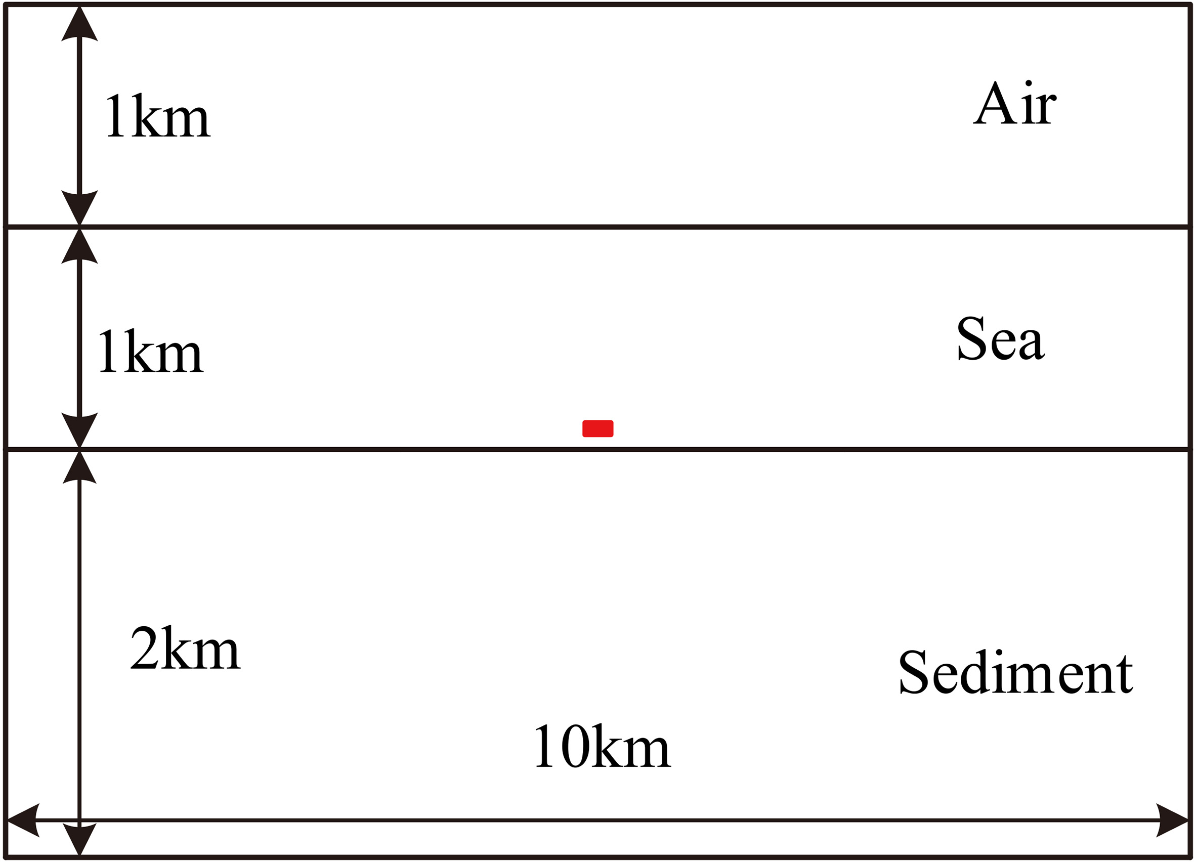$y=$ 0 section of horizontal layered model. The red star in this figure indicates the excitation dipole source.

6.1 Algorithm verification

To validate our algorithm, we consider a horizontally layered geoelectrical model as shown in the Fig. 4. The depth of the air and sea is 1000 m. The conductivity of air, sea water and sediment are set to be 10 ${}^{-6}$ s/m, 3.3 s/m, 0.5 s/m, respectively. The source is a horizontal electric dipole oriented in the $x$ direction with the moment of 100 Am and located in the seawater with the coordinates (0, 0,950) m. The frequency of the harmonic electric source is 0.1 Hz. The semi-analytical solution is calculated by using the fast Hankel transform method [31, 32]. The receive stations at the seafloor ( $z=$ 1000 m). The modeling domain is set to be $\Omega=\{-5∼{}\text{km}\leqslant x,y\leqslant 5∼{}\text{km},-1∼{}\text{km}% \leqslant z\leqslant 3∼{}\text{km}\}$ . The unstructured grid of horizontal layered model as shown in the Fig. 5. Figure 6 shows a comparison between FE result, with three types of edge-elements, and analytical solution. From the Fig. 6, one can see that the finite element results based on three different edge elements agreement well with the analytical solutions. Figure 7 shows the relative error of the Finite element results for different edge-elements. The Table 1 show the efficiency of different elements which are used for MCSEM modeling. From Fig. 7 and Table 1, one can see that the proposed method is more accurate with lower computational cost in comparison to the refined tetrahedral mesh with the 1 ${}^{\text{st}}$ element. Compare to conventional second-order edge element, the efficiency of the proposed method is significantly higher than that of conventional second-order edge element and without loss to much accuracy.

Table 1
The comparison of efficiency of the different elements

Element type	Number of elements	Number of unknowns	IDR(s) iterations	CPU tine (s)
1st order	1,593,700	1,840,769	1957	698
2 ${}^{\text{nd}}$ order	265,431	1,746,023	1632	510
2 ${}^{\text{nd}}$ order (proposed)	265,431	1,396,819	819	285

Figure 5.

The size of unstructured mesh for the 1D model at $y=$ 0 m. the red star in this figure indicates the electric dipole sources.

Figure 6.

A comparison between the FE solution with different edge-elements the analytical solution for the isotropic 1D model.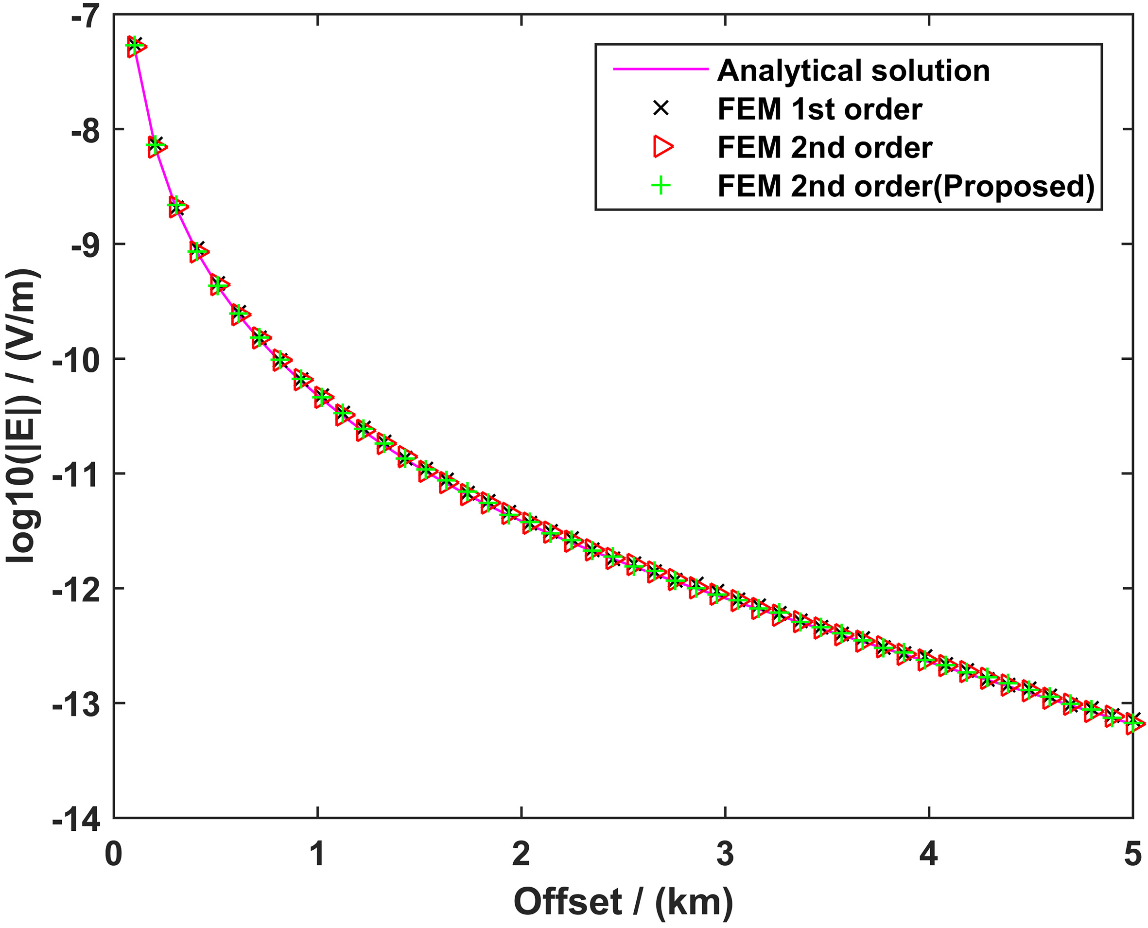

Figure 7.

The relative error of FEM results with different kind of edge-element.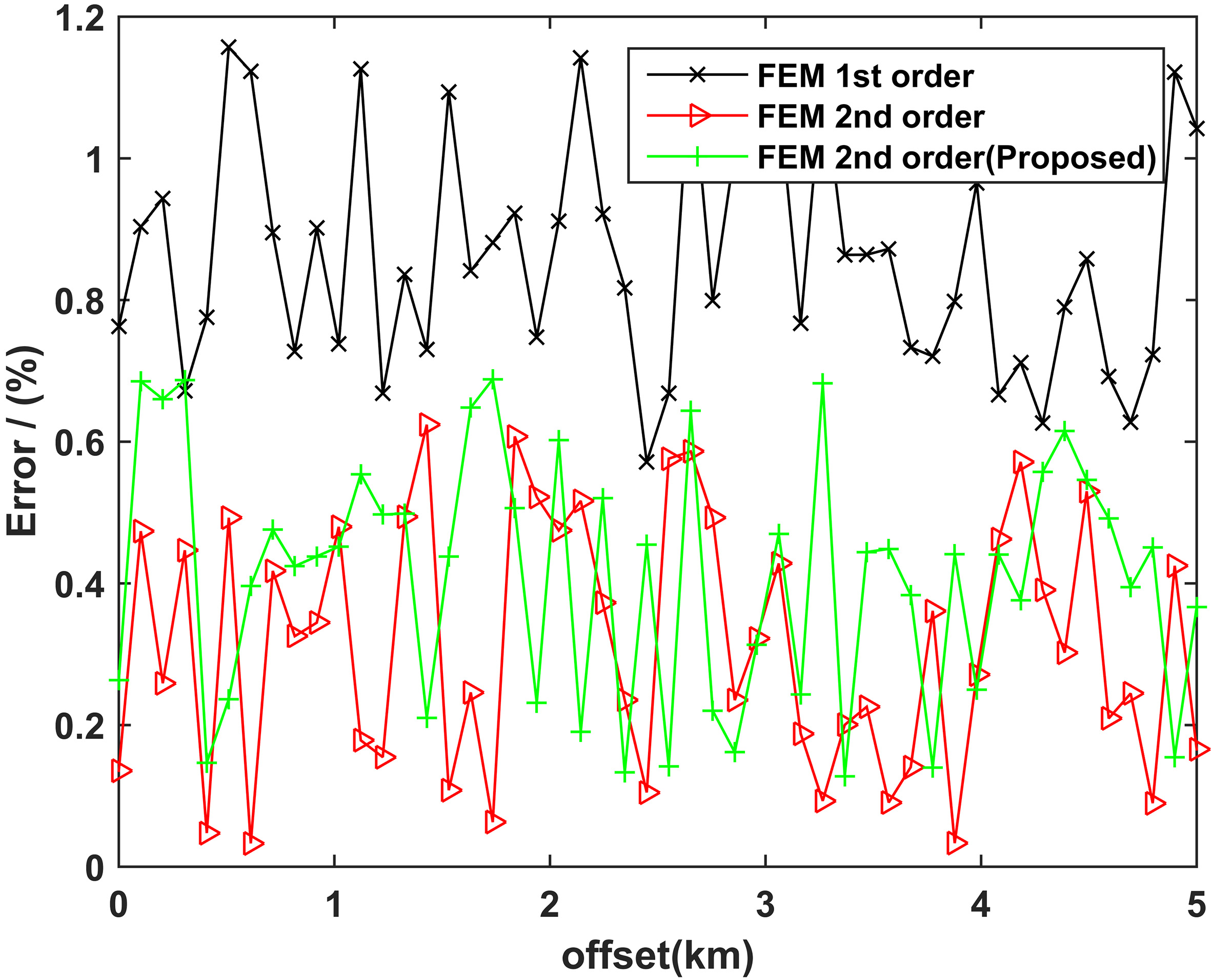

Figure 8.

Vertical section at 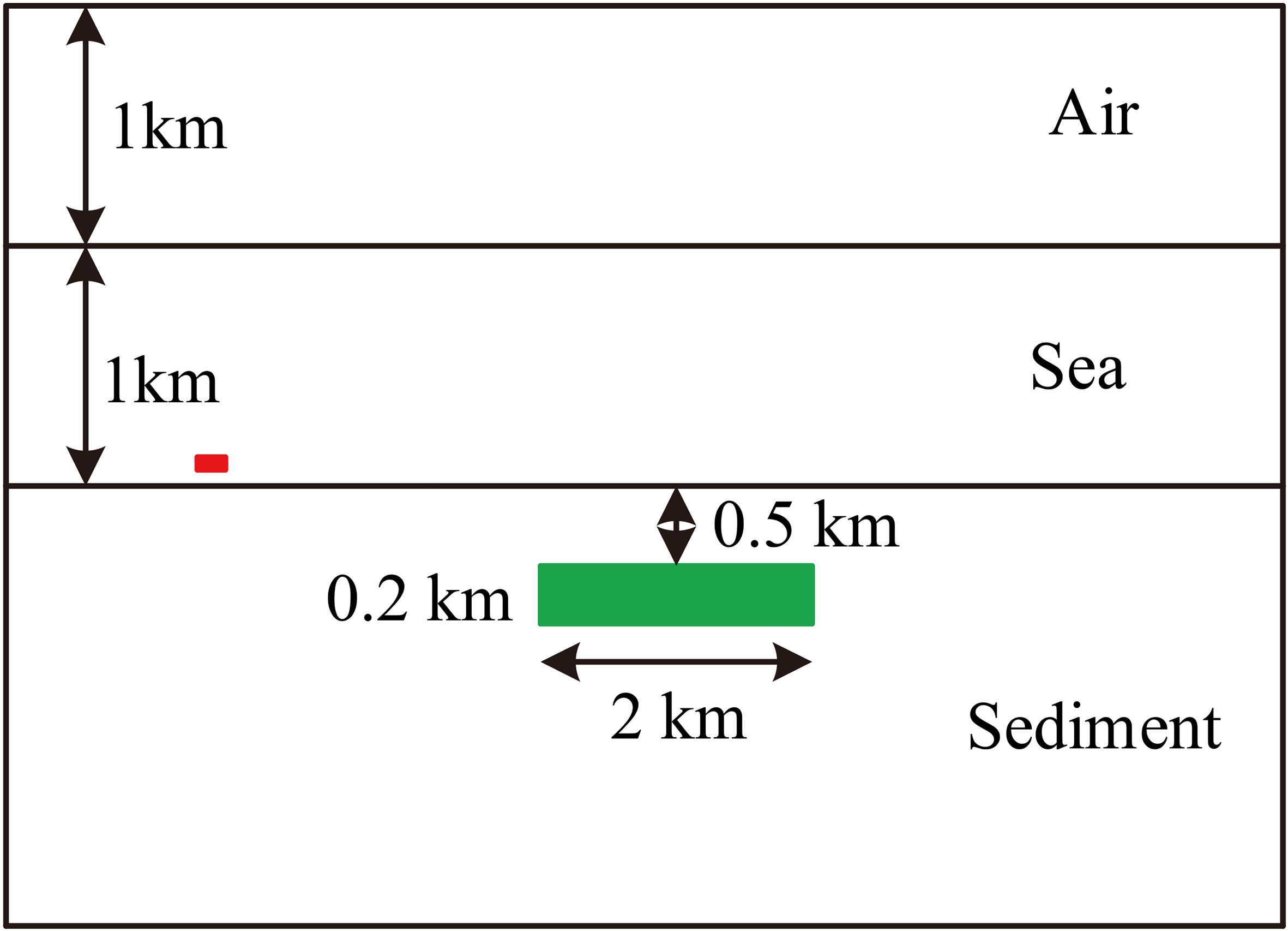$y=$ 0 of model of an off-shore hydrocarbon reservoir. red rectangle denotes the electric dipole source.

6.2 Model of an off-shore hydrocarbon reservoir

In this section, we consider a hydrocarbon reservoir model which is embedded in the sediments as shown in the Figs 8 and 9. The conductivity and depth of sea water and air are the same as the previous model. The horizontal and vertical conductivity of sediment 1 s/m and 0.5 s/m, respectively. The reservoir is isotropic with the conductivity is 0.001 s/m. The size of reservoir is 2 km $\times$ 2 km $\times$ 0.2 km with the central coordinate (1000, 0, 1500) m. The excitation source of the electromagnetic field is the horizontal electric dipole with a moment of 100 Am. The excitation source’s coordinate is ( $-$ 3000, 0, 950) m. The frequency of excitation sources is 1 Hz which is often used in the MCSEM exploration. The modeling domain is set to be $\Omega=\{-5∼{}\text{km}\leqslant x,y\leqslant 5∼{}\text{km},-1∼{}\text{km}% \leqslant z\leqslant 3∼{}\text{km}\}$ . The unstructured grid of hydrocarbon reservoir model as shown in the Fig. 8.

The Figs 10 and 11 show the comparison of anomalous ${Ex}$ field by using different elements for isotropic sediment and anisotropic sediment, respectively. Figures 12 and 13 show the comparison of total and background field for isotropic and anisotropic sediment, respectively. From the Figs 9 and 10, one can find the results of proposed method are in agreement with that of conventional 2 ${}^{\text{nd}}$ edge element. What is more, we can see that the anisotropic background conductivity can significantly influence MCSEM data. The Table 2 show the comparison of efficiency for different elements which are used for MCSEM modeling. One also can see that the efficiency of proposed method is still higher than that of conventional 2 ${}^{\text{nd}}$ edge element.

Table 2
The comparison of efficiency of the different elements

Element type	Number of elements	Number of unknowns	IDR(s) iterations	CPU tine (s)
2 ${}^{\text{nd}}$ order	1,166,068	7,670,473	2132	1124
2 ${}^{\text{nd}}$ order (proposed)	1,166,068	6,136,382	1319	793

Figure 9.

The size of unstructured mesh for the reservoir model at 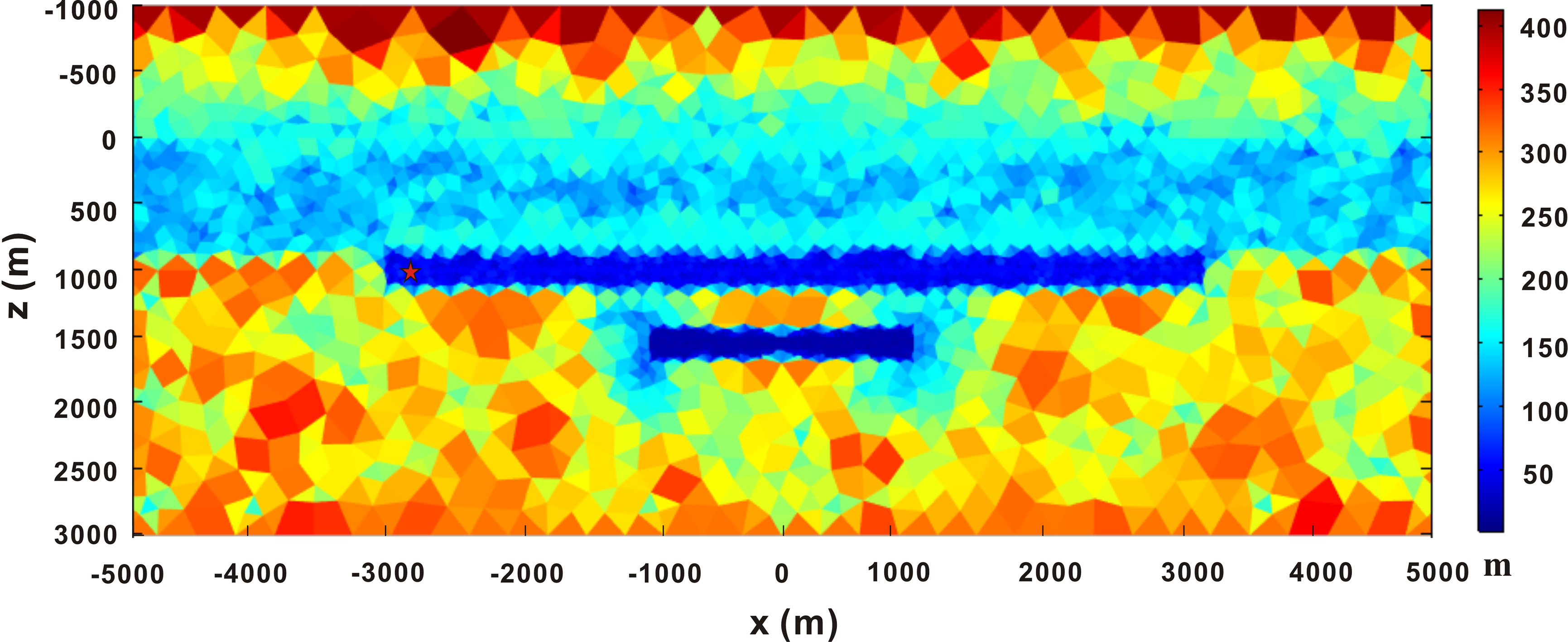$y=$ 0 m, the red star in this figure indicates the excitation dipole source.

Figure 10.

A comparison of the x-component of the anomalous electric field computed using the conventional 2nd tetrahedral elements (blue line) and proposed element for isotropic sediment.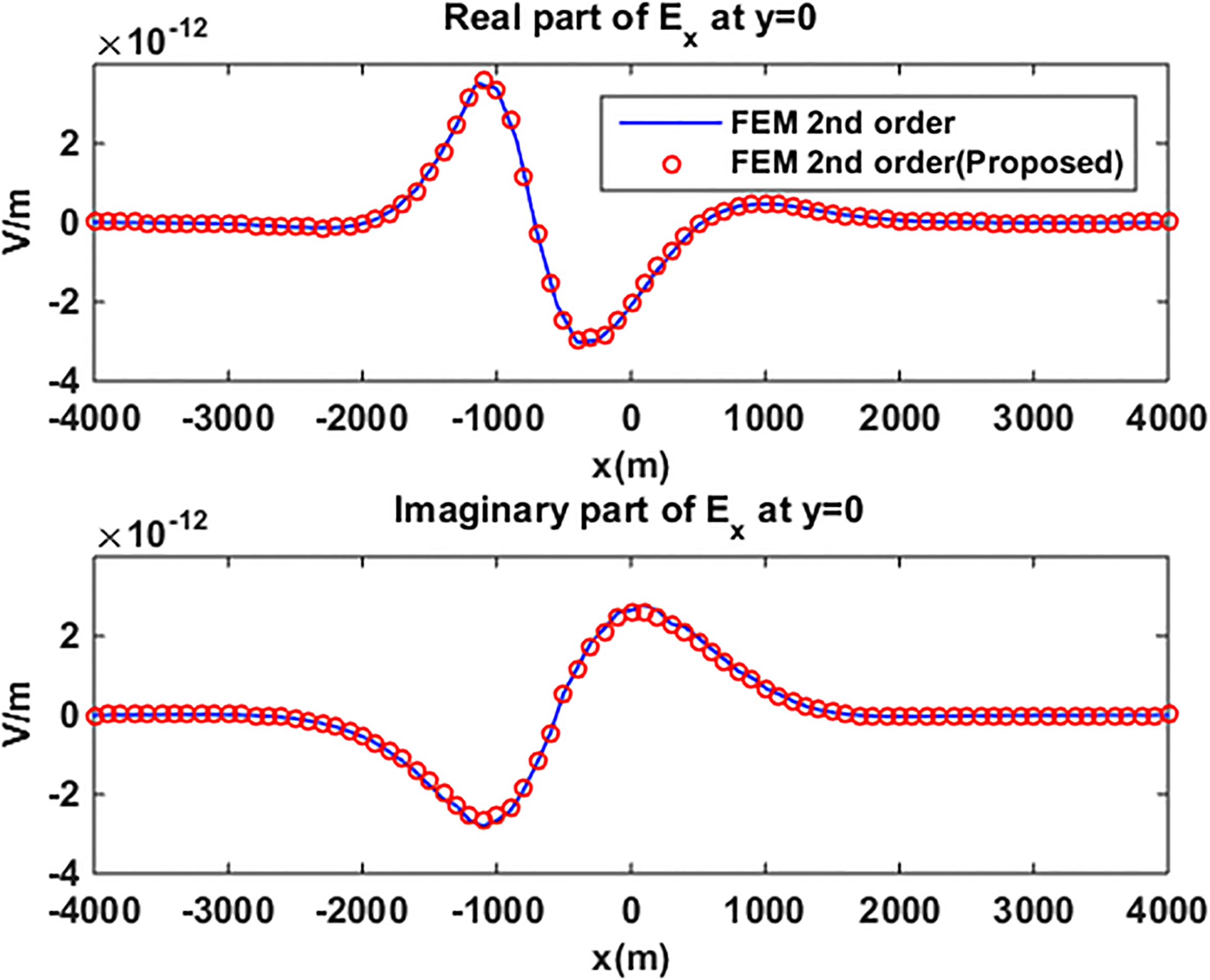

Figure 11.

A comparison of the x-component of the anomalous electric field computed using the conventional 2nd tetrahedral elements (blue line) and proposed element for anisotropic sediment.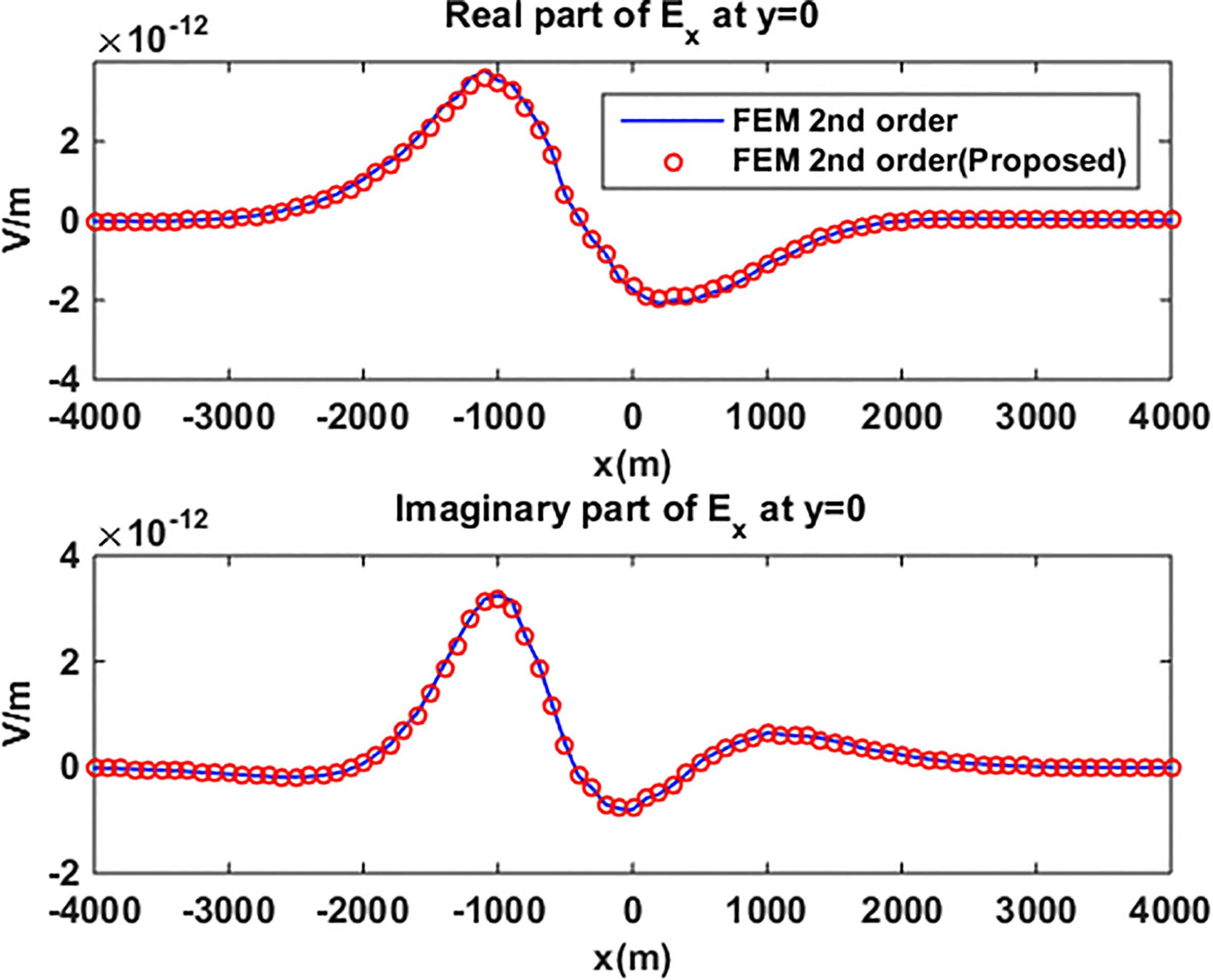

Figure 12.

The comparison of total field and background filed for isotropic sediment.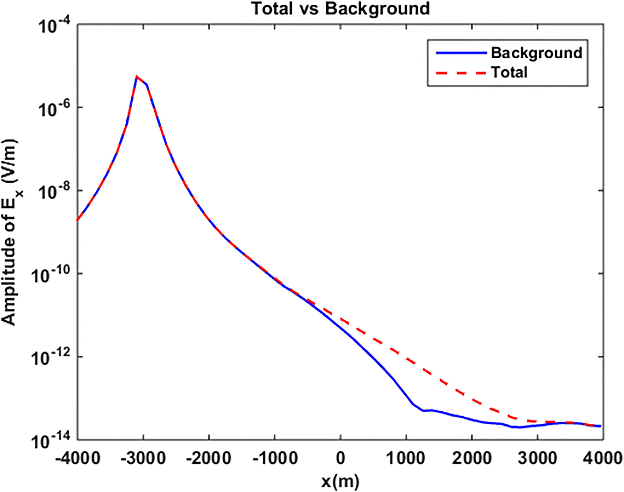

6.3 3D Reservoir model with pyramid-shaped bathymetry

We consider a model with two reservoirs and Pyramid-hill shaped bathymetry as shown in the Fig. 14. The bottom of Pyramid-hill shaped bathymetry is $\Omega=\{-500∼{}\text{m}\leqslant x,y\leqslant 500∼{}\text{m}\}$ . The top of Pyramid-hill shaped bathymetry is $\Omega=\{-250∼{}\text{m}\leqslant x,y\leqslant 250∼{}\text{m}\}$ . Within the area of bathymetry, the seafloor depth changes from 900 m to 1000 m. the depth and conductivity of air and sea water also the same as the previous models. These reservoirs are defined by $\Omega 1=\{-500∼{}\text{m}\leqslant x\leqslant 500∼{}\text{m},-500∼{}\text{m}% \leqslant y\leqslant 500∼{}\text{m},2000∼{}\text{m}\leqslant z\leqslant 2100∼{% }\text{m}\}$ . The modeling domain is set to be $\Omega_{\textit{modeling}}=\{-4∼{}\text{km}\leqslant x\leqslant 4∼{}\text{km},% -3.6∼{}\text{km}\leqslant y\leqslant 3.6∼{}\text{km},-1∼{}\text{km}\leqslant z% \leqslant 4∼{}\text{km}\}$ . The modeling domain is discrete by using the tetrahedron element as shown in the Fig. 15. The grid is refined nearby the source, target layer, bathymetry and the location of observation.

Table 3
The comparison of efficiency of the different elements

Element type	Number of elements	Number of unknowns	IDR(s) iterations	CPU tine (s)
2 ${}^{\text{nd}}$ order	1,366,068	8,986,087	2568	1401
2 ${}^{\text{nd}}$ order (proposed)	1,366,068	7,188,873	1721	911

Figure 13.

The comparison of total field and background filed for anisotropic sediment.

Figure 14.

Vertical section at 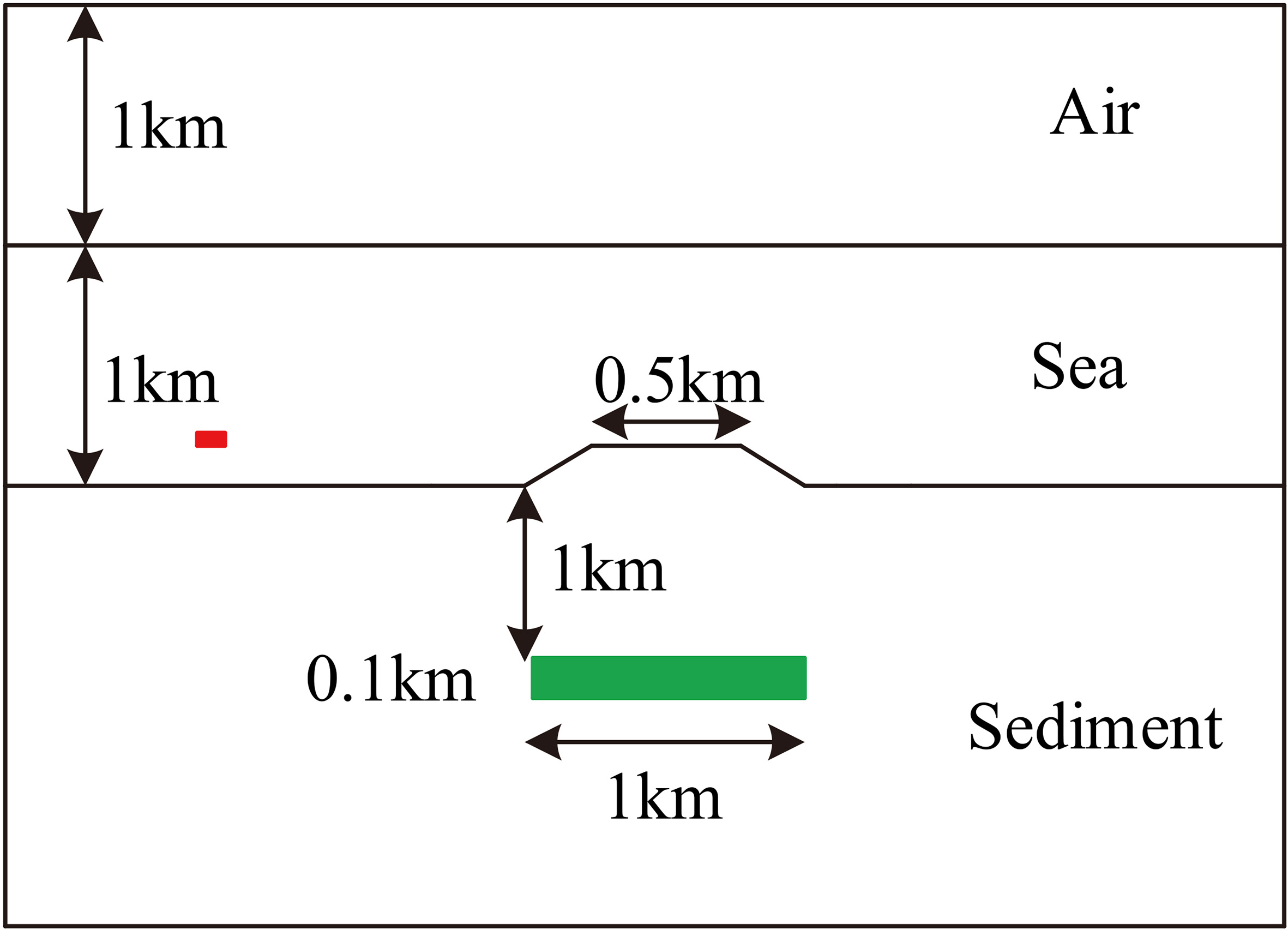$y=$ 0 of 3D Reservoir model with pyramid-shaped bathymetry. The red rectangle denotes the electric dipole source.

Figure 15.

The size of unstructured mesh for the bathymetry model at 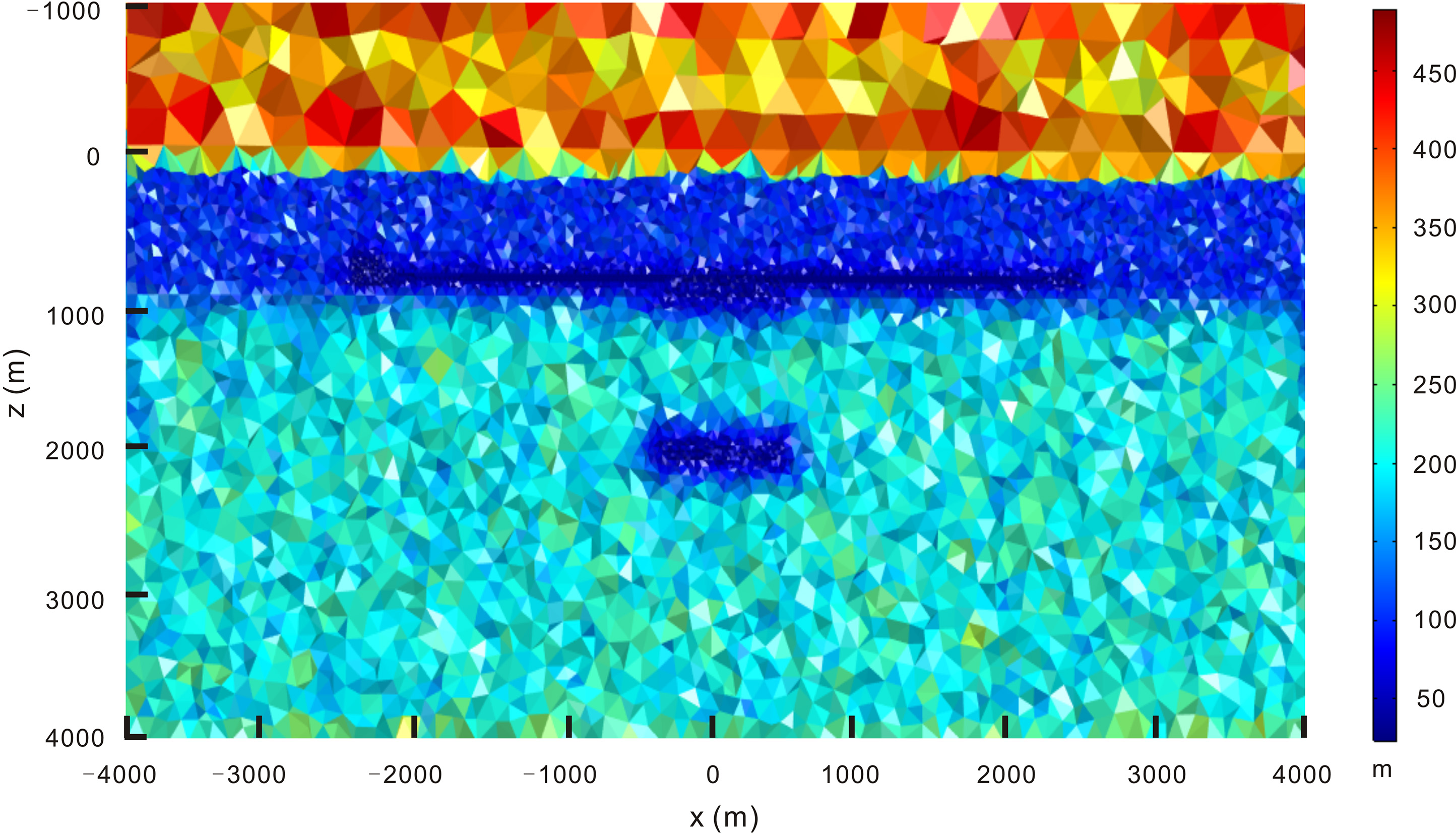$y=$ 0 m, the red star in this figure indicates the excitation dipole source.

Figure 16.

A comparison of the x-component of the anomalous electric field computed using the conventional 2nd tetrahedral elements (blue line) and proposed element for bathymetry model without reservoir.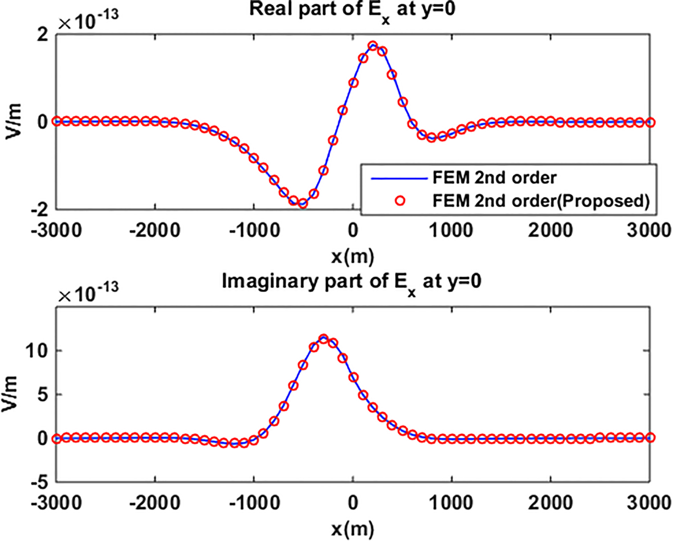

Figure 17.

A comparison of the x-component of the anomalous electric field computed using the conventional 2nd tetrahedral elements (blue line) and proposed element for bathymetry model with a reservoir.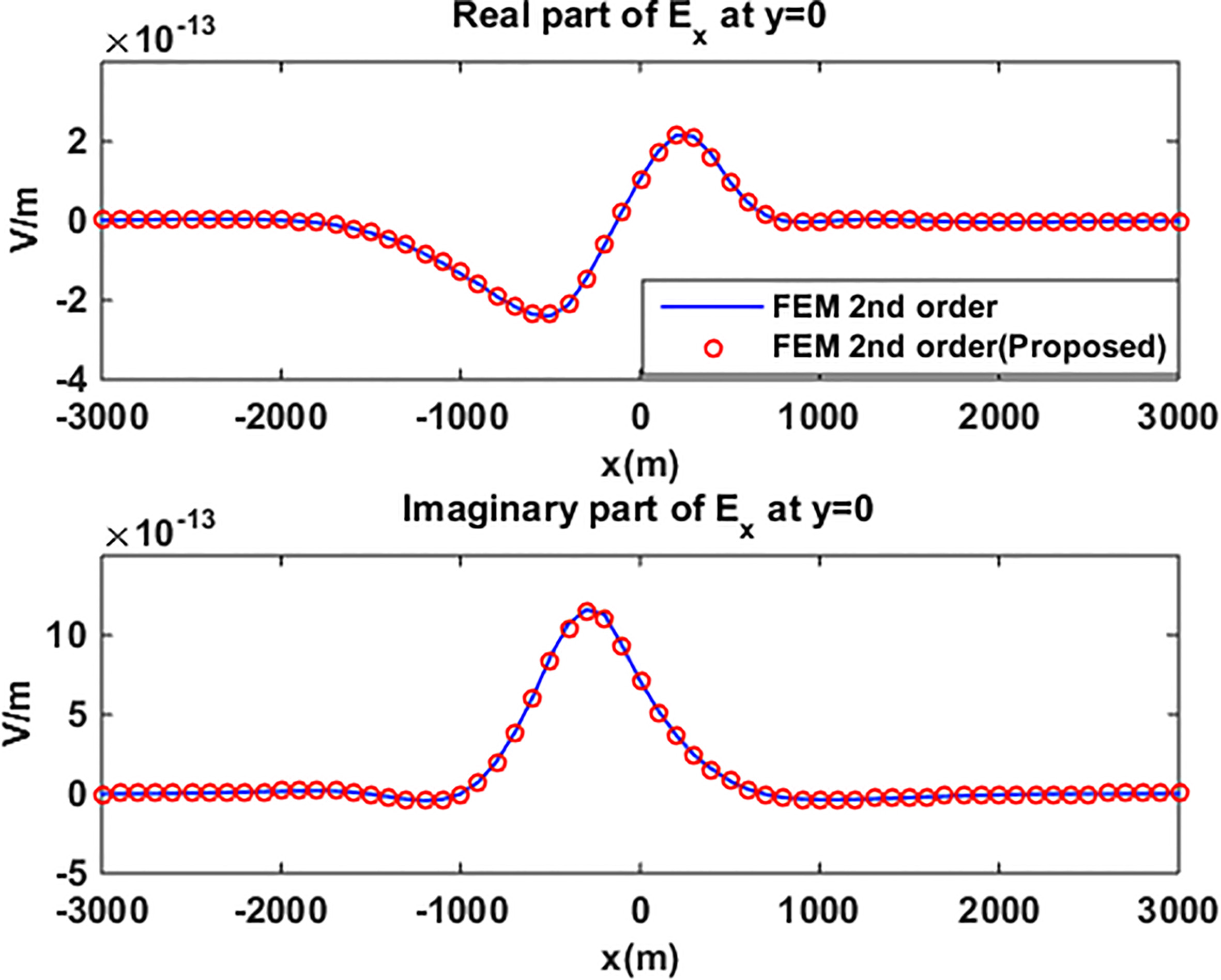

The depth and conductivity of air and sea water still the same as the previous models. The conductivity of the sediment is set to be 1 s/m. The horizontal and vertical conductivities of the reservoir is 0.05 s/m. The excitation source is a horizontal electric dipole with the coordinate of ( $-$ 3500, 0, 900) m. the moment and frequency of source is 100 Am and 1 Hz, respectively.

The Figs 16 and 17 show the comparison of the anomalous electric field computed using the conventional 2 ${}^{\text{nd}}$ tetrahedral elements (blue line) and proposed element for bathymetry model without reservoir and with reservoir, respectively. One can find that the results of two type of elements is still in agreement with each other. In addition, From Figs 16 and 17, one also can see that the bathymetry can significant influence on marine CSEM data. Table 3 shows the comparison of CPU time for proposed method and conventional 2 ${}^{\text{nd}}$ element based FEM. Similar to the previous models, the CPU time of proposed method obviously less than the conventional 2 ${}^{\text{nd}}$ edge-element based FEM.

7. Conclusion

We propose an edge finite element algorithm base on a new type of second order edge element for 3D modeling of MCSEM field. We adopt the anomalous field formulation and the source’s singularity can be avoided effectively. We solve the system of equations using the IDR(s) algorithm with the ILU preconditioner. We validated our algorithm by several models, the modeling results has demonstrated our algorithm enables considerable reduction in computational cost without any loss of accuracy when compared with the edge finite element algorithm based on the conventional first and second order edge elements. The algorithm has good versatility and can be extended for airborne and Land electromagnetic forward modeling.

Footnotes

Acknowledgments

The authors are thankful to the anonymous reviewers and the Editor, Dr. Toshiyuki Takagi for their valuable suggestions that helped to improve the presentation of the paper. The project was partially supported by the project with name “comprehensive study of seismic and magnetic cross-sections in the South China Sea” (grant code: 20162x05026007-001).

References

Hohmann

G.W.

, Three-dimensional induced polarization and electromagnetic modeling, Geophysics 40 (1975), 309–324.

Newman

G.A.

and Hohmann

G.W.

, Transient electromagnetic response of high-contrast prisms in a layered earth, Geophysics 53 (1988), 691–706.

Avdeev

and Knizhnik

, 3D integral equation modeling with a linear dependence on dimensions, Geophysics 74 (2009), F89–F94.

Angiulli

Cacciola

Calcagno

De Carlo

Morabito

C.F.

Sgró

and Versaci

, A numerical study on the performances of the flexible BiCGStab to solve the discretized E-field integral equation, International Journal of Applied Electromagnetics and Mechanics 46(3) (2014), 547–553, doi: 10.3233/JAE-141939.

Mackie

R.M.

Smith

J.T.

and Madden

T.R.

, Three-dimensional electromagnetic modeling using finite difference equations: the magnetotelluric example, Radio Sci. 29 (1994), 923–935.

Newman

G.A.

and Alumbaugh

D.L.

, Frequency-domain modeling of airborne electromagnetic responses using staggered finite differences, Geophys Prospect 43 (1995), 1021–1042.

Haber

Ascher

U.M.

Aruliah

D.M.

and Oldenberg

, Fast simulation of 3D electromagnetic problems using potentials, J. Comput. Phys. 163 (2000), 150–171.

Jahandari

and Farquharson

C.G.

, A finite-volume solution to the geophysical electromagnetic forward problem using unstructured grids, Geophysics 79 (2014), E287–E302.

Jahandari

and Farquharson

C.G.

, Finite-volume modelling of geophysical electromagnetic data on unstructured grids using potentials, Geophys. J. Int. 202 (2015), 1859–1876.

10.

Badea

Everett

Newman

and Biro

, Finite element analysis of controlled-source electromagnetic induction using coulomb-gauged potentials, Geophysics 66 (2001), 786–799.

11.

Schwarzbach

B̈orner

R.U.

and Spitzer

, Three-dimensional adaptive higher order finite element simulation for geo electromagnetics – A marine CSEM example, Geophys. J. Int. 178 (2011), 63–74.

12.

Ansari

and Farquharson

C.G.

, 3D finite-element forward modeling of electromagnetic data using vector and scalar potentials and unstructured grids, Geophysics 79 (2014), E149–E165.

13.

Hussain

Karsiti

M.N.

Jeoti

and Yahya

, Use of wavelets in marine controlled source electromagnetic method for geophysical modeling, International Journal of Applied Electromagnetics and Mechanics (2016), 431–443, doi: 10.3233/JAE-160002.

14.

Cai

Xiong

Han

and Zhdanov

, 3D controlled-source electromagnetic modeling in anisotropic medium using edge-based finite element method, Computers & Geosciences 73 (2014), 164–176.

15.

Cai

Xiong

and Zhdanov

, Three-dimensional marine controlled-source electromagnetic modelling in anisotropic medium using finite element method, Chinese Journal of Geophysics 58 (2015), 2839–2850.

16.

Chen

Wang

and Xiong

, Characteristics analysis of 3D marine CSEM response using the vector finite element method with secondary formulation, International Journal of Applied Electromagnetics and Mechanics (2017), 565–581.

17.

Zhdanov

M.S.

, Geophysical Electromagnetic Theory and Methods, Elsevier, 2009.

18.

Zhdanov

M.S.

Lee

S.K.

and Yoshioka

, Integral equation method for 3D modeling of electromagnetic fields in complex structures with inhomogeneous background conductivity, Geophysics 71 (2006), 333–345.

19.

Streich

, 3D finite-difference frequency-domain modeling of controlled-source electromagnetic data: Direct solution and optimization for high accuracy, Geophysics 74 (2009), F95–F105.

20.

Jin

, Finite Element Method in Electromagnetics, Wiley-IEEE Press, New York, 2002.

21.

Puzyrev

Koldan

Puente

Houzeaux

Vázquez

and Cela

J.M.

, A parallel finite-element method for three-dimensional controlled-source electromagnetic forward modelling, Geophys. J. Int. 193 (2013), 678–693.

22.

Mukherjee

and Everett

M.E.

, 3D controlled-source electromagnetic edge-based finite element modeling of conductive and permeable heterogeneities, Geophysics 76 (2011), F215–F226.

23.

Ansari

and Farquharson

C.G.

, 3D finite-element forward modeling of electromagnetic data using vector and scalar potentials and unstructured grids, Geophysics 79 (2014), E149–E165.

24.

Weiss

and Constable

, Mapping thin resistors and hydrocarbons with marine EM methods: Modeling and analysis in 3D, Geophysics 71 (2006), G321–G332.

25.

Börner

R.U.

Ernst

G.O.

and Spitzer

, Fast 3-D simulation of transient electromagnetic fields by model reduction in the frequency domain using Krylov subspace projection, Geophysical Journal International 173 (2008), 766–780.

26.

Fujiwara

Nakata

and Ohashi

, Improvement of convergence characteristic of ICCG method for the A-ϕ method using edge elements, IEEE Transactions on Magnetics 32 (1996), 804–807.

27.

Dyczij-Edlinger

Peng

and Lee

, A fast vector-potential method using tangentially continuous vector finite elements, IEEE Transactions on Microwave Theory and Techniques 46 (1998), 863–868.

28.

Biró

and Preis

, Partial tree-gauging of second order edge element vector potential formulations, in: Proc. Compumag Conf., Montreal, QC, Canada, Jun./Jul., 2015.

29.

Sonneveld

and van Gijzen

M.B.

, IDR(s): a family of simple and fast algorithms for solving large nonsymmetric systems of linear equations, SIAM J. Sci. Comput 31(2) (2008/09), 1035–1062, doi: 10.1137/070685804.

30.

Saad

, Iterative methods for sparse linear systems: SIAM, 2003.

31.

Ward

S.H.

and Hohmann

G.W.

, Electromagnetic Theory for Geophysical Applications, 1988, SEG, Oklahoma.

32.

Anderson

W.L.

, A hybrid fast Hankel transform algorithm for electromagnetic modeling, Geophysics 54 (1989), 263–266.

An edge-based finite element method for 3D marine controlled-source electromagnetic forward modeling with a new type of second-order tetrahedral edge element

Abstract

Keywords

1. Introduction

2. Theory

2.1 Governing equations

Table 1 The comparison of efficiency of the different elements

Table 2 The comparison of efficiency of the different elements

Table 3 The comparison of efficiency of the different elements

Footnotes

Acknowledgments

References

Table 1
The comparison of efficiency of the different elements

Table 2
The comparison of efficiency of the different elements

Table 3
The comparison of efficiency of the different elements